A Multiple Local Models Approach to Accuracy Improvement in Continuous Glucose Monitoring

Introduction

S elf-monitoring of blood glucose is recognized as a milestone of diabetes care since the 1980s, allowing for improvement of metabolic control, especially in insulin-treated patients. ¹ This has prompted research in the field of continuous glucose monitoring (CGM) with a growing body of evidence, although not definite, that it might translate into better glycemic control compared with self-monitoring of blood glucose. ² However, the accuracy of currently available CGM devices is relatively poor, especially in the hypoglycemic range, where the false-positive and false-negative rates are unacceptably high. ^{3 –5} Although small improvements have been achieved with the newest sensor generations, ^6,7 this is a critical issue because accurate prediction of plasma glucose (PG) is strongly needed in diabetes subjects before these systems are largely used either for glucose monitoring only or with the aim of “closing the loop” for a regulated insulin infusion by a minipump in the future.

Current commercially available CGM systems for home monitoring are subcutaneous electrochemical sensors. All of them use the glucose oxidase enzyme–based technology, which give a measure of glucose concentration into the interstitial fluid in terms of intensity of the current generated from the enzymatic reaction (expressed in nA). ⁸ This means that a CGM system actually needs calibration against concurrent blood glucose values, thus providing an estimate of blood glucose concentration.

Actually, the current intensity from subcutaneous glucose sensors is the result not only of the interstitial glucose concentration, but also of the complex interaction between the sensor and the subject. Therefore the accuracy of the estimation of blood glucose from the measurement in the interstitial fluid will depend, among other factors, on the calibration algorithm. Indeed, the latter is a function that includes the relationship between PG and the sensor signal from interstitial fluid glucose, trying to minimize physiological differences between the two compartments. Unfortunately, however, few studies have systematically investigated this relationship, ^{9 –14} with heterogeneous results. This highlights the complexity of the PG-to-interstitial glucose dynamics and of the subject-to-sensor interaction, which contrasts with the rather simplistic approach of calibration algorithms currently implemented in commercial CGM systems ¹⁵ (basically linear regression methods).

Indeed, linear regression models implemented in a CGM system usually require calibration under conditions of relative glycemic stability (at “stationary” metabolic states) where equilibrium between PG and interstitial glucose is expected. In this way, the relationship between the measured current intensity and PG is considered static, and both the plasma to interstitium transport dynamics and the possibly subject–specific sensor interaction are neglected. This has been recognized as a limitation of currently calibration algorithms, but only a few authors have proposed alternative calibrations strategies, ^{16 –18} each one with some practical limitations that prevent its application to clinical practice. ¹⁹

An alternative approach is to consider that the relationship between PG and the sensor signal from interstitial glucose is not linear and likely depends on the metabolic status. In this case, accurate estimation of PG requires mathematical models describing the relationship between PG and the electrical signal generated by interstitial fluid glucose concentrations, during both steady-state and dynamic conditions. ^{16 –18}

The aim of this article is to describe a new calibration algorithm based on the integration of several local dynamic models, each one valid in a specific region, to estimate the PG level from measurements in a remote compartment (in this case, the interstitial space). The use of multiple local models (LMs) allows for a better description of the complexity of the PG to interstitial glucose dynamics, improving the accuracy of the estimations. Suitability and performance of this new technique are tested with a data set from a clinical study, where the sensor's current signal, glucose estimates, and paired reference PG measurement are available. Results are expressed in terms of accuracy of glucose estimates from the new calibration algorithm and compared with those obtained with the standard calibration procedure.

Methods

The proposed algorithm ²⁰ has been developed and validated using data from eu-, hypo-, and hyperglycemic clamps, where healthy subjects wore a microdialysis-based glucose sensor (GlucoDay^®, A. Menarini, Florence, Italy). The study has been described in detail elsewhere. ²¹ In brief, after an initial period of spontaneous euglycemia, at time +30 min an insulin infusion was started, at the rate of 1 mU/kg/min, and continued until 120 min. At the same time, glucose (20% [wt/vol] dextrose) was infused when necessary at a variable rate allowing for a controlled slow fall of PG in about 60 min, until the target of approximately 50 mg/dL was reached. From time +90 min to +120 min PG was maintained at a hypoglycemic plateau of approximately 50 mg/dL. At time +120 min insulin infusion was stopped, and the glucose infusion rate was increased to raise PG after 45 min to the target of approximately 165 mg/dL (time +165 min), which was maintained for the next 15 min until time +180 min. PG was measured every 6 min synchronously with the output of the sensor, which gave a glucose estimate every 3 min.

Principles of the new calibration algorithm

The algorithm is based on a model that describes the relationship between PG concentrations and the signal from the sensor. The structure of the model is described in detail elsewhere. ²² Basically, it is based on the integration of several LMs (Fig. 1), each one characterized by independency and regional validity, in order to obtain an interpretable global model (GM): \documentclass{aastex}\usepackage{amsbsy}\usepackage{amsfonts}\usepackage{amssymb}\usepackage{bm}\usepackage{mathrsfs}\usepackage{pifont}\usepackage{stmaryrd}\usepackage{textcomp}\usepackage{portland,xspace}\usepackage{amsmath,amsxtra}\pagestyle{empty}\DeclareMathSizes{10}{9}{7}{6} \begin{document} \begin{align*} GM = \sum_{i = 1}^c WLM_i \tag{1} \end{align*} \end{document}

OPEN IN VIEWER

FIG. 1.

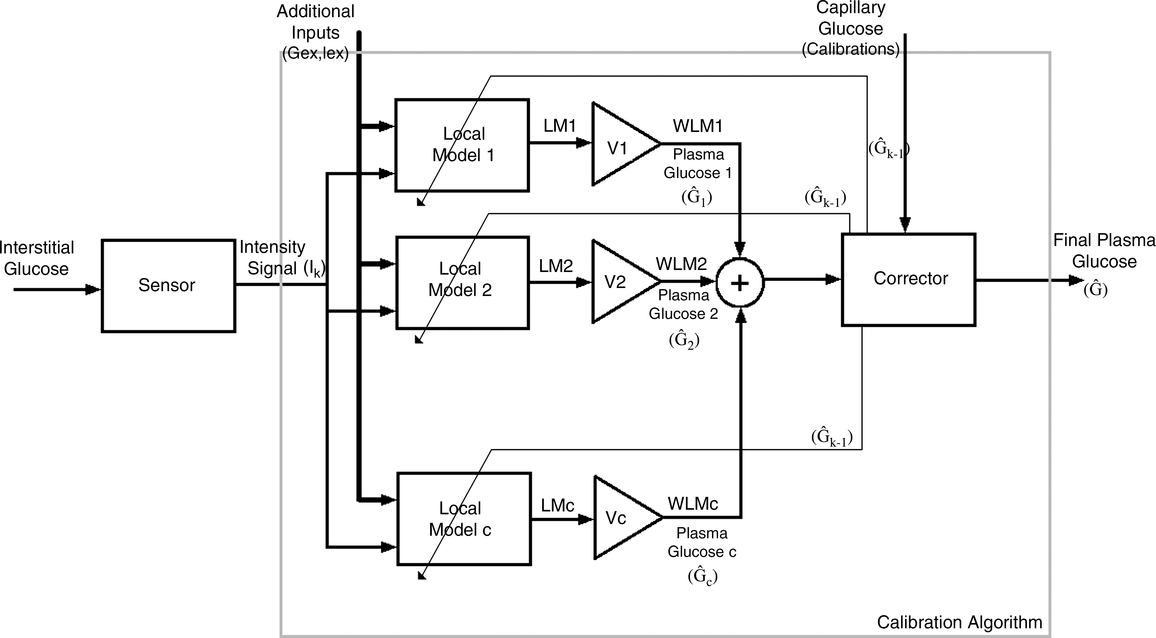
Inputs from a remote compartment, in this case the interstitial space, feed the calibration algorithm. The basic inputs include I_k , I_{k -1}, and Ĝ_{k -1} (current and past intensity value from the sensor and past glucose estimation, respectively) and define both which local models (LMs) and to what extent they are valid. The latter is achieved weighing each LM by a validity function V_i and minimizing both local and global errors. Weighed LMs (WLMs) are added, resulting in the global model, which provides the global glucose estimation. A block to consider the calibration point(s) from capillary measurements is included to correct the estimation of the algorithm. If available, additional signals can also be included (presence/absence of insulin or glucose infusion, meal, exercise, etc.).

where WLM_i is the weighted LM i. Each weighted LM, WLM_i , is the result of the LM LM_i multiplied by its validity function V_i : \documentclass{aastex}\usepackage{amsbsy}\usepackage{amsfonts}\usepackage{amssymb}\usepackage{bm}\usepackage{mathrsfs}\usepackage{pifont}\usepackage{stmaryrd}\usepackage{textcomp}\usepackage{portland,xspace}\usepackage{amsmath,amsxtra}\pagestyle{empty}\DeclareMathSizes{10}{9}{7}{6} \begin{document} \begin{align*} WLM_i = V_i \cdot LM_i \tag{2} \end{align*} \end{document}

The structure of each LM could be any, but in this calibration algorithm linear models are used to add interpretability to the GM: \documentclass{aastex}\usepackage{amsbsy}\usepackage{amsfonts}\usepackage{amssymb}\usepackage{bm}\usepackage{mathrsfs}\usepackage{pifont}\usepackage{stmaryrd}\usepackage{textcomp}\usepackage{portland,xspace}\usepackage{amsmath,amsxtra}\pagestyle{empty}\DeclareMathSizes{10}{9}{7}{6} \begin{document} \begin{align*} LM_i = \beta_{1i} \cdot x_1 + \beta_{2i} \cdot x_2 + \ldots + \beta_{Di} \cdot x_D + \beta_{0i} = \beta_{1D_i} \cdot x_{1D} + \beta_{0i} \tag{3} \end{align*} \end{document}

where x _1D is the D-dimensional vector of inputs of the system and [β_1D , β_0i ] is the D+1-dimensional vector of the regression coefficients β of each linear LM with β ₀ an independent term.

As represented in Eq. 2, each LM is weighted by some validity functions (V_i ) that, in the proposed algorithm, are chosen to be hyper-Gaussian functions. ²³ They are normalized in order to define the degree of validity of the i ^th LM in the input's space so that V_i =1 if the i ^th LM is 100% representative of the current input; in contrast, V_i =0 if the i ^th LM does not characterize the current input at all. Equations 4 and 5 show the final normalized hyper-Gaussian validity function for the one-dimensional and multidimensional cases, respectively: \documentclass{aastex}\usepackage{amsbsy}\usepackage{amsfonts}\usepackage{amssymb}\usepackage{bm}\usepackage{mathrsfs}\usepackage{pifont}\usepackage{stmaryrd}\usepackage{textcomp}\usepackage{portland,xspace}\usepackage{amsmath,amsxtra}\pagestyle{empty}\DeclareMathSizes{10}{9}{7}{6} \begin{document} \begin{align*} \begin{split} \quad V_i = e^{-\frac {1} {2} \left( \left( \frac {x - m_i} {\sigma_i} \right) ^2 \right) ^H} \end{split} \tag{4} \end{align*} \end{document} \documentclass{aastex}\usepackage{amsbsy}\usepackage{amsfonts}\usepackage{amssymb}\usepackage{bm}\usepackage{mathrsfs}\usepackage{pifont}\usepackage{stmaryrd}\usepackage{textcomp}\usepackage{portland,xspace}\usepackage{amsmath,amsxtra}\pagestyle{empty}\DeclareMathSizes{10}{9}{7}{6} \begin{document} \begin{align*} V_i = e^{-\frac {1} {2} \left( (\vec x - \vec m_i) ^T \Sigma_i^{- 1} (\vec x - \vec m_i) \right) ^H} \tag{5} \end{align*} \end{document}

where x is the input and m_i and σ_i are the center and the SD, respectively, of the i ^th validity function. For the multidimensional case, \documentclass{aastex}\usepackage{amsbsy}\usepackage{amsfonts}\usepackage{amssymb}\usepackage{bm}\usepackage{mathrsfs}\usepackage{pifont}\usepackage{stmaryrd}\usepackage{textcomp}\usepackage{portland,xspace}\usepackage{amsmath,amsxtra}\pagestyle{empty}\DeclareMathSizes{10}{9}{7}{6} \begin{document}$$\vec x$$\end{document} and \documentclass{aastex}\usepackage{amsbsy}\usepackage{amsfonts}\usepackage{amssymb}\usepackage{bm}\usepackage{mathrsfs}\usepackage{pifont}\usepackage{stmaryrd}\usepackage{textcomp}\usepackage{portland,xspace}\usepackage{amsmath,amsxtra}\pagestyle{empty}\DeclareMathSizes{10}{9}{7}{6} \begin{document}$$\vec m$$\end{document} are vectors, T refers to the transposed vector, and _Σ is the diagonal matrix of variances of each validity function: \documentclass{aastex}\usepackage{amsbsy}\usepackage{amsfonts}\usepackage{amssymb}\usepackage{bm}\usepackage{mathrsfs}\usepackage{pifont}\usepackage{stmaryrd}\usepackage{textcomp}\usepackage{portland,xspace}\usepackage{amsmath,amsxtra}\pagestyle{empty}\DeclareMathSizes{10}{9}{7}{6} \begin{document} \begin{align*} \Sigma = \left [ \begin{matrix} \sigma_1^2 & 0 & 0 & 0 \\ 0 & \sigma_2^2 & 0 & 0 \\ & & \ddots & \\ 0 & 0 & 0 & \sigma_D^2 \end{matrix}\right ] \end{align*} \end{document}

The use of hyper-Gaussian functions allows the algorithm to find compact regions where an LM is valid. Moreover, the number of parameters to define the model is reduced because only two parameters have to be defined for each input x_j and each LM: mean (m_ij ) and variance (σ ² _ij ). Validity functions are independent functions, making each LM independent as well. This facilitates finding LMs defined by different characteristics of the inputs (i.e., different dynamics representative of the relationship between interstitial glucose and PG influenced by the interaction sensor/subject).

In summary, the resulting model will be described by a set of parameters: the regression coefficients of the linear models and the means and variances of the hyper-Gaussian membership functions, all of them defined for each LM. The final structure of the model can be seen in Eq. 6, already adapted for the D-dimensional case: \documentclass{aastex}\usepackage{amsbsy}\usepackage{amsfonts}\usepackage{amssymb}\usepackage{bm}\usepackage{mathrsfs}\usepackage{pifont}\usepackage{stmaryrd}\usepackage{textcomp}\usepackage{portland,xspace}\usepackage{amsmath,amsxtra}\pagestyle{empty}\DeclareMathSizes{10}{9}{7}{6} \begin{document} \begin{align*}GM = \sum_ { i = 1 } ^c \left( e^ { - \frac { 1 }{ 2 } \left( (\vec x - \vec m_i) ^T \Sigma_i^ { - 1 } (\vec x - \vec m_i) \right) ^H } \cdot \big( \beta_ { 1D_i } \cdot x + \beta_ { 0i } \big) \right) \tag { 6 } \end{align*} \end{document}

The total number of parameters to identify will only depend on the number of inputs considered and on the number of LMs.

An additional feature of the proposed algorithm is that it is structured to minimize both the error of the glucose estimation from each LM (the difference between each LM's glucose estimation and reference glucose [local error]) and the error of the GM (the difference between the GM's glucose estimation and reference glucose [global error]). Optimal LM and validity function parameters are obtained through global optimization of a cost index comprising global and local errors. However, greater importance is given to the accuracy of glucose estimation from each LM compared with the accuracy of the GM. ²¹ This strengthens the ability of the algorithm to find LM valid regionally, with each one characterizing to a different degree (0% to 100%) different PG to interstitial glucose dynamics and/or sensor–subject interactions.

Finally, it is worth mentioning that, as the calibration algorithm may use inputs of different nature, normalization is required to make them all have, a priori, the same weight in the modeling process.

Glucose estimation given by the model is corrected every time a new calibration point is introduced, updating past values.

Results

Figure 2 shows PG estimates obtained with the new algorithm, in the configuration not accounting for binary signals, compared with reference PG measurements. On the other hand, the output of each one of the two LMs composing the GM (already weighted by its validity function) can be seen in Figure 3. Figure 2 shows that the estimated signal is quite close to the reference glucose for all patients, indicating good performance of the algorithm even in this case with no exogenous information and only two LMs. Figure 3 shows that each one of the two LMs represents only a subset of the study subjects (LM₁ for subjects 5 and 6 vs. LM₂ for the remaining subjects), whereas only the weighted integration of both LMs to form the GM allows for glucose estimations very close to the actual concentrations (Fig. 2) in the whole population.

OPEN IN VIEWER

FIG. 2.

Comparison between global glucose estimation (G _e [solid line]) and paired available reference glucose (G _r [dotted line]), plotted by each patient and each 6-min sample (dots). This is for the basic input vector, called IIG, and for only two local models (c=2). These signals have also been compared with the original manufacturer's sensor accuracy (G _s).

OPEN IN VIEWER

FIG. 3.

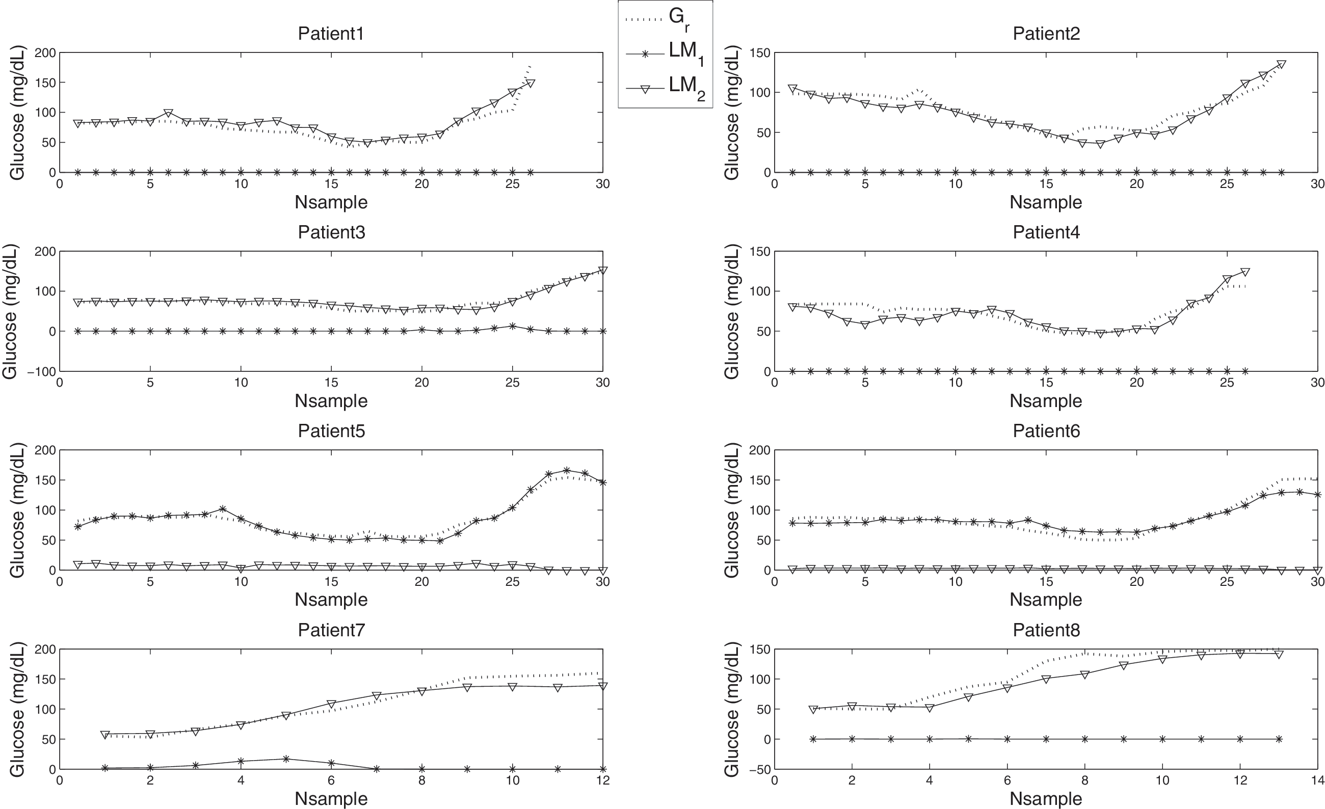
Comparison between the reference glucose (G _r) and the estimation of glucose done only by each local model (LM₁ and LM₂). This is for the basic input vector (IIG) and for c=2. It can be seen how LM₁ provides accurate plasma glucose estimations just for Patients 5 and 6, whereas this local estimation does not contribute at all to the accuracy of the estimation in the rest of patients. On the other hand, LM₂ provides accurate plasma glucose estimations in all but patients 5 and 6, where its contribution to the accuracy of the estimation is nearly 0.

Table 1 shows the performance of the proposed algorithm both in its “basic” configuration and considering information from binary signals [i.e., the presence (I _ex,G _ex=1) or absence (I _ex,G _ex=0) of insulin and/or glucose infusion]. The comparison with the results from the one-point calibration implemented by the GlucoDay demonstrates that the new calibration algorithm allows for a significant improvement of the accuracy of the glucose estimations. In particular, the inclusion of additional information about the metabolic status further improves the accuracy of glucose estimations, reducing the MARD and M2ARD below 10%. It is noteworthy that the magnitude of improvement was similar for both the whole and the hypoglycemic range. However, likely because of the small sample size, under conditions of hypoglycemia the difference did not reach statistical significance.

Conclusions

This study describes and validates a new calibration algorithm for CGM systems, based on a dynamic model that includes the relationship between PG levels and measurements in a remote compartment (in this case, the interstitial space). The strength and novelty of this method reside in the structure of the GM, which is composed by several LMs weighted and added together. LMs are defined by a validity function and a linear combination of the inputs, so that each one represents to a variable extent a different (metabolic) condition and/or sensor–subject interaction. Then, each subject will be represented by one or more LMs, and the shift from one LM to another is defined by the inputs (i.e., the output of the sensor but also every other signal containing information relevant to the glucose dynamic). It is noteworthy that each LM has a very simple structure (linear), favoring interpretability of the GM. Moreover, the validity function of LMs (V_i ) makes LMs representative of very specific and well-defined regions on the input space, allowing for the identification of the regions they represent. All these may help to elucidate the relationship between the signal(s) from the remote compartment and PG levels, describing different glucose dynamics and sensor behaviors. It does mean that this calibration algorithm can be applied to any sensor that offers some indirect measurement related to PG levels, with the number and parameters of each LM being determined by the particular sensor's output.

When PG is estimated from direct or indirect measurements in any compartment alternative to blood, the following information should be ideally included into the calibration algorithm in order to improve the accuracy of glucose estimations: (1) the intrinsic dynamic of the sensor, (2) glucose dynamic between plasma and the remote compartment, and (3) factors influencing the previous two dynamics. Indeed, sensors of different nature, or even sensors belonging to the same class, may each have a specific intrinsic dynamic. In this regard, recently it has been shown how much of the lag time of continuous glucose sensors is in fact due to the intrinsic delay in the sensor response to changes in glucose concentrations. ²⁶ Additionally, the interaction between a sensor and the remote compartment of measurement is likely to be specific: in the case of minimally invasive sensors (which to date are the only commercially available) it depends on the biocompatibility of the materials used and on the inflammatory reaction following its insertion. This relationship is complex, may be time-dependent (as the foreign body reaction progresses), and certainly is specific to each individual. ^27,28

However, to date the issue of enhanced calibration algorithm has received poor attention with only a few scientific contributions. Knobbe and Buckingham ¹⁶ were the first who considered intercompartmental glucose dynamics and developed a five-state extended Kalman filter for the estimation of subcutaneous glucose levels. Facchinetti et al. ¹⁸ further developed the strategy proposed by Knobbe and Buckingham ¹⁶ and proposed the “enhanced Bayesian calibration method” based on an extended Kalman filter estimating interstitial glucose, PG, and sensor sensitivity along time. The method is intended to be used in cascade to any calibration algorithm built in commercial CGM devices and was validated on simulated data representative of diabetes subjects, showing improved CGM accuracy compared with the method of Knobbe and Buckingham. ¹⁶ However, a drawback of this validation is the use of the same model of interstitial glucose and sensor sensitivity for data generation and state estimation, although in the first case a robustness analysis considering discrepancies in lag time estimation is conducted. Furthermore, as the authors acknowledge, application of the enhanced Bayesian calibration method to real data has two main limitations: first, it requires the knowledge of the variances of both state and measurement processes, which in real-life conditions are unknown; second, the existence of a burn-in period, considered as one day by the authors.

Leal et al. ²⁹ considered sensor and glucose dynamics using a different approach. In particular, autoregressive techniques were applied to CGMS^® System Gold^™ (Medtronic, Northridge, CA) to monitor data from a clinical study in patients with diabetes. A third-order model of the relationship between current intensity given by the monitor and reference PG measurements was obtained. Predictions given by the model were corrected at every calibration point introduced by the patient, and a cross-validation analysis yielded a substantial improvement of the accuracy of glucose estimations. ²⁸ However, a drawback of autoregressive models is that frequent recalibration may be needed to ensure a good performance.

At variance with the previous approaches, the proposed calibration algorithm, thanks to its structure of LMs, is better suited to find and correct for all the above-mentioned dynamics, improving the accuracy of glucose estimations. Results from the present study should be considered as a proof of concept. Indeed, in the small population studied at least two different dynamics of the sensor-to-subject interaction were found, each one detected by a different LM: LM₁ for subjects 5 and 6 and LM₂ for the other subjects. The reason for the existence of two different LMs was easily explained by analysis of the electric signal from the sensors. Although PG and insulin concentrations were very similar in all subjects (it was a clamp study), there were two “clusters” of current intensity, with the one from sensors inserted in subjects 5 and 6 being much smaller compared with the other. This could be probably due to differences in sensor sensitivity, which were captured automatically by the algorithm. Consideration of both dynamics by means of the two independent LMs allowed for a significant improvement of glucose estimations compared with the original algorithm implemented by the GlucoDay. Additionally, the proposed algorithm admits the introduction of information about the metabolic condition of the subject as a binary signal. This further improved the accuracy of the glucose estimation and appears to be an interesting feature because any information potentially relevant to the sensor-to-subject interaction (physical activity/inactivity, fed/fasting state, etc.) can be used to feed the algorithm.

However, the study has three main limitations. (1) The study population is composed by just eight healthy subjects, and data should be considered preliminary. Thus it is quite probable that the structure of the obtained algorithm is not representative of the general population of people with diabetes. Indeed, getting a calibration algorithm applicable to the general population of people with diabetes would require a specific clinical study in a representative sample, and validation of the obtained algorithm should be carried out in a different study involving larger numbers of subjects with both type 1 and type 2 diabetes. However, in this case the structure of the proposed algorithm is not expected to change regarding the inputs to be considered, although more LMs would probably be needed to cover the greater heterogeneity of local behaviors. (2) Data from reference PG measurement are available for a limited time for each subject. This could in theory have reduced the possibility of identifying different glucose dynamics and sensor behaviors. However, during the clamp study, glucose and insulin concentrations varied through all the clinical significant ranges of eu-, hypo-, and hyperglycemia, giving a good picture of the changes observed in real-life conditions. In contrast, longer studies should be performed to identify changes in the dynamics of the sensor over time, avoiding underestimation of the number c of LMs needed to describe the PG/remote compartment glucose relationship. This is particularly true for minimally invasive sensors where biofouling, inflammation, and foreign body reaction (which are probably tissue and subject specific) induce changes in the sensor's response to variations in glucose concentration. (3) Finally, to prove robustness of the algorithm to cope with variability, the results must be confirmed in a sample representative of the population of patients with diabetes. In this regard, from a phylogenetic point of view it is expected that the inter-subject variations in the intercompartmental glucose dynamics, as well as the spectrum of the inflammatory responses to the sensor's insertion, are limited. However, because of changes in the microcirculation, the variability of the sensor-to-subject interaction (i.e., different sensor sensitivities, sensor's drift overtime, metabolic conditions, etc.) might be greater in patients with diabetes, especially those with microvascular complications. ³⁰ Nevertheless, the accuracy of CGM in patients with diabetes seems to be not different compared with healthy subjects, indicating that the theoretical greater variability associated with the diabetes condition may have limited practical impact.

Despite its limitations, in this proof-of-concept study the LMs technique is demonstrated to be an effective approach for CGM calibration algorithms. Indeed, aside the very good results obtained in terms of accuracy of glucose estimations, the short computational time associated with this methodology makes it feasible for real-time monitoring and implementation in every glucose sensor.