Hypo- and Hyperglycemia in Relation to the Mean,Standard Deviation,Coefficient of Variation,and Nature of the Glucose Distribution

Abstract

Aims:

We describe a new approach to estimate the risks of hypo- and hyperglycemia based on the mean and SD of the glucose distribution using optional transformations of the glucose scale to achieve a more nearly symmetrical and Gaussian distribution, if necessary. We examine the correlation of risks of hypo- and hyperglycemia calculated using different glucose thresholds and the relationships of these risks to the mean glucose, SD, and percentage coefficient of variation (%CV).

Materials and Methods:

Using representative continuous glucose monitoring datasets, one can predict the risk of glucose values above or below any arbitrary threshold if the glucose distribution is Gaussian or can be transformed to be Gaussian. Symmetry and gaussianness can be tested objectively and used to optimize the transformation.

Results:

The method performs well with excellent correlation of predicted and observed risks of hypo- or hyperglycemia for individual subjects by time of day or for a specified range of dates. One can compare observed and calculated risks of hypo- and hyperglycemia for a series of thresholds considering their uncertainties. Thresholds such as 80 mg/dL can be used as surrogates for thresholds such as 50 mg/dL. We observe a high correlation of risk of hypoglycemia with %CV and illustrate the theoretical basis for that relationship.

Conclusions:

One can estimate the historical risks of hypo- and hyperglycemia by time of day, date, day of the week, or range of dates, using any specified thresholds. Risks of hypoglycemia with one threshold (e.g., 80 mg/dL) can be used as an effective surrogate marker for hypoglycemia at other thresholds (e.g., 50 mg/dL). These estimates of risk can be useful in research studies and in the clinical care of patients with diabetes.

Introduction

C linical care might be improved if clinicians could obtain reasonably reliable estimates of the risks of hypo- and hyperglycemia by time of day, in relationship to meals, by day of the week, by longitudinal date, and for various combinations of these factors for any given patient. These estimates have usually been estimated as the probability of an event using empirically observed rates, often based on a very small number of observed events. Random sampling errors for a proportion are large when there are few events, as is usually the case in the “tails” of a distribution (e.g., for glucose <50 or <40 mg/dL or for glucose >250 or >400 mg/dL). For example, with n=20 observations and four events, the probability of an event is 0.20 or 20%, but the 95% confidence interval for that estimate range from 2% to 38%, a 19-fold range. When events are rare, use of a count of events provides only limited information and is an inefficient method to characterize the nature of the distribution. We sought to develop and apply a method that can provide more precise estimates by analyzing the entire distribution rather than just the rare events in the tails of the distribution.

Kovatchev et al.¹ introduced a transformation of the glucose scale to achieve a (nearly) symmetrical distribution and demonstrated a high correlation of the Low Blood Glucose Index with subsequent risk of severe hypoglycemia.^1,2 Monnier et al.³ reported a relationship between risk of hypoglycemia and the magnitude of the percentage coefficient of variation (%CV) for glucose; in contrast, the risk of hyperglycemia was related to the mean and SD of glucose values, but only minimally to the %CV. Qu et al.⁴ and Inzucchi et al.⁵ have made similar observations. Swinnen et al.⁶ noted that the rates of hypoglycemia depend on the arbitrary choice of glucose level used as the criterion for hypoglycemia.

Principle of the present method

If glucose data were subject to a “Gaussian” or “normal” distribution, then one could accurately predict the probability of hypoglycemic or hyperglycemic events if we knew the true population mean and SD. However, the distribution of glucose values is usually non-Gaussian,^1,7 the exact nature of the distribution is unknown, and one is subject to random sampling errors in the sample mean and sample SD.⁸ In the present study, we propose to use simple nonlinear transformations of the glucose scale to achieve an approximation to the Gaussian distribution, which in turn permits estimation of the risks of hypo- or hyperglycemia using any desired threshold.⁹ This principle should be applicable to both continuous glucose monitoring (CGM) and self-monitoring of blood glucose when sufficient data are available.

Materials and Methods

Box 1 provides an overview of the proposed method. We first evaluate whether the glucose distribution is consistent with a Gaussian distribution. If not, we attempt to transform the glucose scale to achieve a nearly Gaussian distribution. One can then estimate the probabilities of hypo- or hyperglycemia below or above any arbitrary threshold.⁹ These estimates can be compared with the empirically observed rates for the same dataset. One can evaluate the robustness or stability of results by considering the uncertainties in the mean and SD^8,9 and in the nature of the transformation used for the glucose scale.

Box 1. Simplified Schematic of the Proposed Method to Estimate the Probabilities of Hypo- or Hyperglycemia Using Any Desired Threshold

1. Compute Sample Mean, Sample SD (s), Skew, and Excess Kurtosis of glucose distribution or subsets of the distribution by date, time of day, day of week

2. Perform tests of gaussianness

a. Test whether Skew and Excess Kurtosis are statistically significantly different from zero

b. Wilk–Shapiro test

c. Evaluate gaussianness using one or more graphical methods (e.g., Normality Plot, Q-Q plot, probit plot, or “inverse error function of cumulative frequency distribution” [erf ⁻¹(cfd)] vs. glucose)

3. Apply log and root transforms of the form: \documentclass{aastex}\usepackage{amsbsy}\usepackage{amsfonts}\usepackage{amssymb}\usepackage{bm}\usepackage{mathrsfs}\usepackage{pifont}\usepackage{stmaryrd}\usepackage{textcomp}\usepackage{portland, xspace}\usepackage{amsmath, amsxtra}\pagestyle{empty}\DeclareMathSizes{10}{9}{7}{6}\begin{document}\begin{align*}G^\prime = \log_{10} ( Glucose + c ) \; \hbox{or} \; G^\prime = ( Glucose + c ) ^{ ( 1 / n ) }\end{align*}\end{document}

4. Retest for gaussianness: Identify the optimal values for c, or c and n, to achieve as close to a Gaussian distribution as possible

5. Select desired thresholds for hypo- and hyperglycemia

6. Compute expected probability of glucose below or above the specified thresholds

7. Compare the calculated values for risks of hypo- and hyperglycemia with the empirically observed frequencies of hypoand hyperglycemia using the same thresholds

8. Evaluate robustness of results: consider the uncertainty due to random sampling variability in the sample mean (SEM) and in the sample SD, [SE(s)], and due to the uncertainties in the values for c and n. Consider alternative types of transformations to achieve gaussianness.

9. Display the observed and predicted risks of hypo- or hyperglycemia for a given subject for the entire dataset or versus time of day, day of the week, date, or other variables of interest (e.g., Fig. 2), or compare observed and predicted risks for multiple subjects (e.g., Fig. 3)

One can examine the nature of the glucose distribution by calculating the mean, SD, Skew (a measure of asymmetry), and Kurtosis (a measure of curve shape—“pointiness” or flatness)^9

–14. One can then transform the data using various nonlinear transformations, for example, the log transform after first applying a linear translation to the original glucose scale \documentclass{aastex}\usepackage{amsbsy}\usepackage{amsfonts}\usepackage{amssymb}\usepackage{bm}\usepackage{mathrsfs}\usepackage{pifont}\usepackage{stmaryrd}\usepackage{textcomp}\usepackage{portland, xspace}\usepackage{amsmath, amsxtra}\pagestyle{empty}\DeclareMathSizes{10}{9}{7}{6}\begin{document}\begin{align*}G^\prime = \log_{10} ( Glucose + c ) \tag{1}\end{align*}\end{document}

or the root transform \documentclass{aastex}\usepackage{amsbsy}\usepackage{amsfonts}\usepackage{amssymb}\usepackage{bm}\usepackage{mathrsfs}\usepackage{pifont}\usepackage{stmaryrd}\usepackage{textcomp}\usepackage{portland, xspace}\usepackage{amsmath, amsxtra}\pagestyle{empty}\DeclareMathSizes{10}{9}{7}{6}\begin{document}\begin{align*}G^\prime = ( Glucose + c ) ^{ ( 1 / n ) } \tag{2}\end{align*}\end{document}

For example, if n=2, this would be the square-root transformation of (Glucose+c).

We seek to find values of the constants (c in Eq. 1 or c and n in Eq. 2) that will result in as nearly symmetrical a distribution as possible. For a Gaussian distribution, Skew and Excess Kurtosis should be zero. If the distribution is skewed to the right, as usually the case for glucose, Skew will be positive. If the distribution is skewed to the left, as usually the case for log(Glucose), Skew will be negative. By plotting Skew and Excess Kurtosis versus c and n and estimating the values the values of c and n that result in Skew and Excess Kurtosis as close to zero as possible, one can identify the parameters for the transformations (Eq. 1 or 2) that result in a nearly Gaussian distribution. Alternatively, one can use the Wilk–Shapiro test¹⁰ and/or other criteria to optimize the approximation to gaussianness. Once the best values for the constants in a transformation have been determined, one can recalculate the mean, SD, Skew, and Excess Kurtosis for the transformed glucose values and repeat tests for gaussianness. Several graphical methods are also available to compare an observed distribution with a Gaussian distribution. These include the Normality Plot or a Q-Q plot,^11,12 the probit plot,¹³ or a plot of “inverse error function” of the cumulative frequency distribution (cfd), [erf ^–1(cfd)] versus Glucose or G′.¹⁴

After identifying a transformation such that the transformed glucose data are nearly Gaussian, it becomes possible to estimate the percentage of observations that fall below or above any arbitrary threshold using standard tables and equations for a Gaussian distribution^11,14 (cf. Supplementary Data available online at www.liebertpub.com/dia). One can calculate the probability of a hypoglycemic or hyperglycemic event, using any desired threshold T (e.g., T=40, 50, 60, 70, or 80 mg/dL for hypoglycemia, T=180, 200, 250, 300, or 400 mg/dL for hyperglycemia, or the corresponding values on the transformed glucose scale [T ^′]), using the estimates for mean and SD. The mean and SD can be calculated for the entire dataset or for specified time segments in terms of longitudinal dates, time of day, or day of week. The calculated probabilities of a hyper- or hypoglycemic event can then be displayed versus date, times of day, or days of the week. These are “historical probabilities” based on previous data and may be applied to future dates if one assumes that the underlying temporal process is stable.

To evaluate the robustness of the method, to consider the effects of random sampling errors in the sample mean and sample SD, one can repeat the above calculations and reconstruct the profiles for probability of hypo- or hyperglycemia (e.g., vs. date or vs. time of day) using two plausible values for the Mean combined with two values for the SD, resulting in four combinations of parameters: the two values for the Mean could be selected as \documentclass{aastex}\usepackage{amsbsy}\usepackage{amsfonts}\usepackage{amssymb}\usepackage{bm}\usepackage{mathrsfs}\usepackage{pifont}\usepackage{stmaryrd}\usepackage{textcomp}\usepackage{portland, xspace}\usepackage{amsmath, amsxtra}\pagestyle{empty}\DeclareMathSizes{10}{9}{7}{6}\begin{document}$$\{ \overline { \rm {X}} - t \ { \rm SEM} \} , \ \{ \overline {\rm {X}} + t \ { \rm SEM} \} ;$$\end{document} the two values for the SD ( s ) might be { s – t SE( s )}, { s +t SE( s )}, where SEM is the standard error of the mean, SE( s ) is the SE of the sample SD, and t is the Student's t value for the desired probability level (e.g., t is approximately 0.67, 1, or 2 for 50%, 68%, or 95% confidence intervals, respectively).

The SE of the sample mean is s /√N, where N is the number of observations in the sample. The SE of the sample SD is given approximately⁸ by s /√(2N).

This approach makes it possible to evaluate the effects of uncertainty and random sampling errors in the sample mean and sample SD. However, this does not provide protection from errors that arise from a systematically non-Gaussian distribution. One can evaluate the robustness of results with respect to this potential source of error by repeating the calculations using the untransformed glucose values (assuming that the glucose distribution were Gaussian), using the log transformation with c=0 (i.e., assuming that the glucose values were log-normally distributed), and using an intermediate case where one assumes that the values for log₁₀(Glucose+c) are normally distributed, using the value of c that minimizes Skew. Results for profiles of risk of hypo- and hyperglycemia can then be compared by displaying them simultaneously versus date, time of day, or other variables of interest.

Another approach to evaluation of the robustness of results would be to consider alternative methods for calculation of the sample mean and sample SD. These values \documentclass{aastex}\usepackage{amsbsy}\usepackage{amsfonts}\usepackage{amssymb}\usepackage{bm}\usepackage{mathrsfs}\usepackage{pifont}\usepackage{stmaryrd}\usepackage{textcomp}\usepackage{portland, xspace}\usepackage{amsmath, amsxtra}\pagestyle{empty}\DeclareMathSizes{10}{9}{7}{6}\begin{document}$$( \overline {{ \rm X}} , s )$$\end{document} may be based on the entire dataset (which might involve days, weeks, or months of data) or on the values from a single week, a single day, or a single hour during the day. The larger the set of data used, the more reliable the estimate of \documentclass{aastex}\usepackage{amsbsy}\usepackage{amsfonts}\usepackage{amssymb}\usepackage{bm}\usepackage{mathrsfs}\usepackage{pifont}\usepackage{stmaryrd}\usepackage{textcomp}\usepackage{portland, xspace}\usepackage{amsmath, amsxtra}\pagestyle{empty}\DeclareMathSizes{10}{9}{7}{6}\begin{document}$$\overline {{ \rm X}}$$\end{document} and s . However, the larger the dataset, the greater the risk that the data may be heterogeneous and that the temporal process is unstable. (Combining glucose data from pre- and postprandial time periods is likely to increase skew of the glucose distribution. Use of a narrow time window [e.g., 2 h before breakfast] often results in a smaller SD and a smaller Skew.) The mean glucose and SD may vary with time. For example, the fasting plasma or interstitial fluid glucose might have a between-day SD_b of 15 mg/dL, whereas the after-dinner glucose peak might have a between-day SD_b of 30 mg/dL.^15,16 Similarly, the nature of the glucose distribution may also change with time, such that Skew and Kurtosis may vary with time. Accordingly, the nature of the best transformation of the glucose scale to achieve symmetry and gaussianness may also change with time.

We have evaluated the performance of this method using illustrative data from 64 subjects with type 1 diabetes and 17 subjects with type 2 diabetes using either an insulin pump or multiple daily injections,¹⁷ comparing the observed risks of hypo- and hyperglycemia with those calculated using the present approach using four thresholds (50, 80, 180, and 250 mg/dL). We examined the relationships between observed rates of hypoglycemia <50 mg/dL and observed rates <80 mg/dL, and between observed rates of hyperglycemia >250 mg/dL and >180 mg/dL. We also evaluated the relationship of %CV of glucose with the observed rates of hypoglycemia at two threshold levels (<50 and <80 mg/dL).

Results

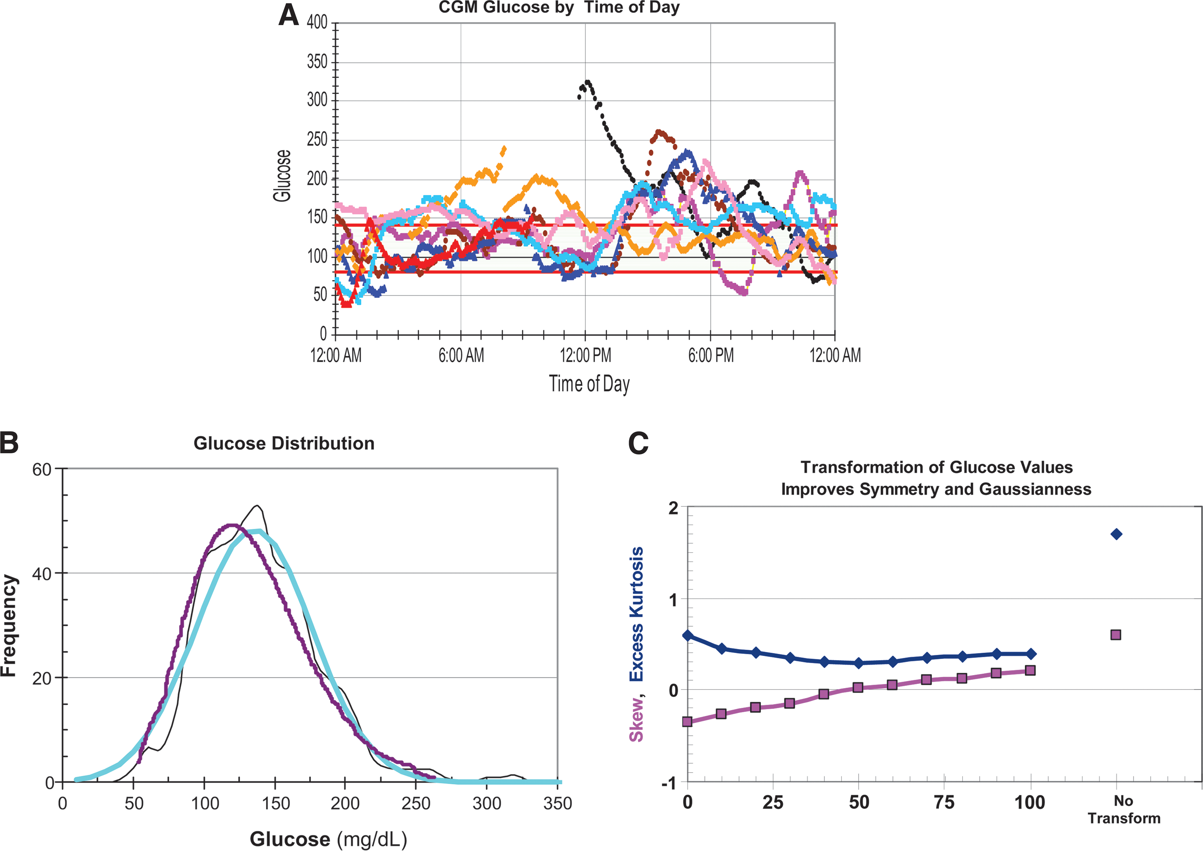
Figures 1 and 2 show results from analysis of CGM data from a single subject. Figure 1A shows representative CGM tracings for a subject for a period of 1 week aligned by time of day as shown in Rodbard et al.¹⁷ However, it is difficult to estimate the risk of hypoglycemia by time of day from this type of “glucose profile”. Figure 1B shows the observed, moderately asymmetrical glucose distribution (frequency histogram) (black curve). A Gaussian distribution with the same mean and SD (blue curve) would systematically overestimate the frequency of hypoglycemia but underestimate the frequency of hyperglycemia. If one transforms the glucose scale so that the glucose distribution becomes more symmetrical, here using log₁₀(Glucose+50 mg/dL), fits a Gaussian distribution to the transformed glucose values, and then redisplays the distribution on the original glucose scale, one can obtain a better approximation to the observed data, especially in the hypoglycemic range (red curve). Figure 1C shows the values for Skew and Excess Kurtosis for the original glucose data (before transformation) and shows how these values change systematically as one adjusts the value of c in the log transformation (Eq. 1). This enables us to identify the value for c that minimizes Skew: c=50 mg/dL in the present example. (In the author's experience with multiple datasets, a value of c between 30 and 50 mg/dL often results in considerably improved symmetry of the glucose distribution.)

FIG. 1.

(A) Representative continuous glucose monitoring (CGM) data for a period of 1 week, with data from successive days superimposed in the form of a “glucose profile.” (B) Histogram (frequency distribution) for glucose from entire dataset (black curve). A Gaussian distribution with the same mean and SD (blue curve) overestimates the probability of glucose values falling below 50 mg/dL and underestimates the probability of glucose values falling above 235 mg/dL. By transforming the glucose scale to achieve a more nearly symmetrical and Gaussian distribution, one obtains and improved fit to the observed distribution (purple curve). (C) Relationship of Skew and Excess Kurtosis to the adjustable parameter c when transforming the glucose scale using the equation G ^′=log₁₀(Glucose+c). For a Gaussian distribution Skew and Excess Kurtosis would both be zero. In this example, it was possible to achieve a Skew of zero and a minimal value of Excess Kurtosis when c is set to 50 mg/dL. Skew and Excess Kurtosis are also shown for the original glucose data (“No Transform”). In this manner, one can select parameters for a transformation to optimize symmetry and gaussianness. The optimal value for c is likely to vary between patients and may vary between datasets within patients, between days, or even between different time segments during the day. Ideally both Skew and Excess Kurtosis would be zero. It is more important to minimize Skew than to minimize Excess Kurtosis, in part because Kurtosis has a larger uncertainty (SE) than Skew. (Excess Kurtosis=Kurtosis−3).

FIG. 2.

Calculated probabilities of hypoglycemia and hyperglycemia by time of day, based on the assumption that glucose has a Gaussian distribution and using the observed values for sample mean \documentclass{aastex}\usepackage{amsbsy}\usepackage{amsfonts}\usepackage{amssymb}\usepackage{bm}\usepackage{mathrsfs}\usepackage{pifont}\usepackage{stmaryrd}\usepackage{textcomp}\usepackage{portland, xspace}\usepackage{amsmath, amsxtra}\pagestyle{empty}\DeclareMathSizes{10}{9}{7}{6}\begin{document}$$\overline {{ \rm X}}$$\end{document} and sample SD ( s ). (A) Calculated probabilities that a glucose value will fall below 80, 70, 60, 50, or 40 mg/dL, by time of day (from top downward: green, turquoise, light blue, blue, and black, respectively). Note the similar patterns observed for all five thresholds. (B) Calculated probabilities that a glucose value will be above 140, 180, or 250 mg/dL, by time of day (from top downward: red, orange, and light orange, respectively). Similar patterns were observed for all three thresholds. (C) Calculated probabilities of hypoglycemia (A) and hyperglycemia (B) are displayed simultaneously: (left axis) probability of a glucose level falling below a specified value and (right scale) probability that a glucose value will fall above a specified value. From top downward: calculated probability that a glucose value is below 250, 180, 140, 80, 70, 60, 50 or 40 mg/dL (red, orange, light orange, green, turquoise, light blue, blue, black, respectively). For the top three curves, the probability of being above the specified threshold is the vertical distance between the position on the curve and the 100% mark. The distance between the green curve (for 80 mg/dL) and the light orange curve (for 180 mg/dL) is the probability of being within a target range of 80–180 mg/dL. This display of predicted risk is closely related to, but distinct from the “stacked bar chart” that has been proposed as a method to display the observed probabilities that a glucose value will fall within any specified range.^18,19 (D) Risk of hypoglycemia <70 mg/dL (left axis) and hyperglycemia >180 mg/dL (right axis) calculated using the observed Mean and SD ( s ) (orange circles and turquoise squares, respectively), the (Mean+1 SEM) or (Mean−1 SEM) (red), [ s +1 SE( s )] or [ s −1 SE ( s )] (green), a logarithmic transform of glucose (blue), and the empirically observed risks of hypo- and hyperglycemia (pink).

Estimation of the risk of hypo- and hyperglycemia based on a Gaussian distribution for glucose (G) or a transformed glucose value (G ^′)

After achieving a Gaussian or nearly Gaussian distribution for glucose (or for a transformed glucose scale), it becomes possible to estimate the probability that a glucose value would be observed below or above any specified threshold.

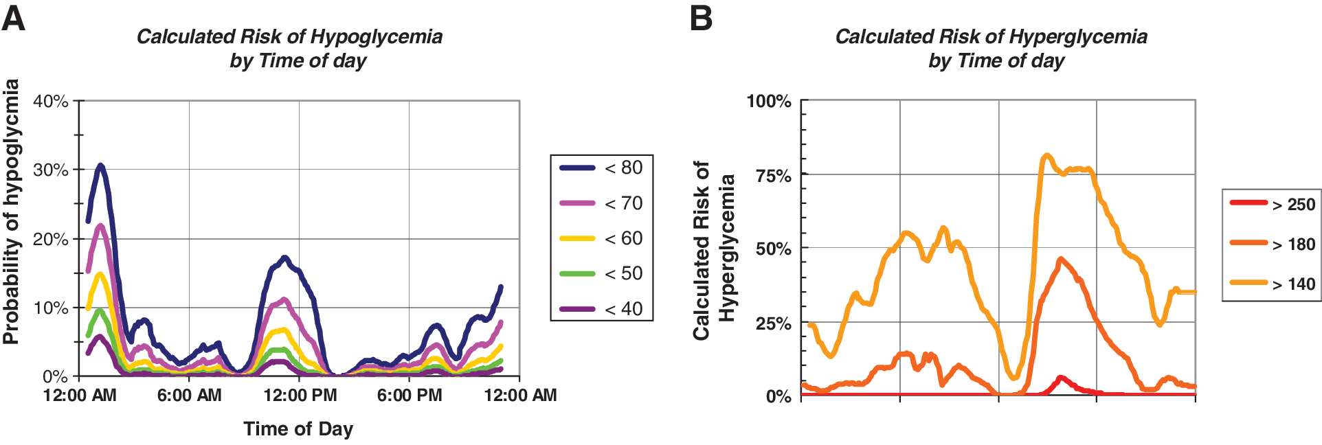
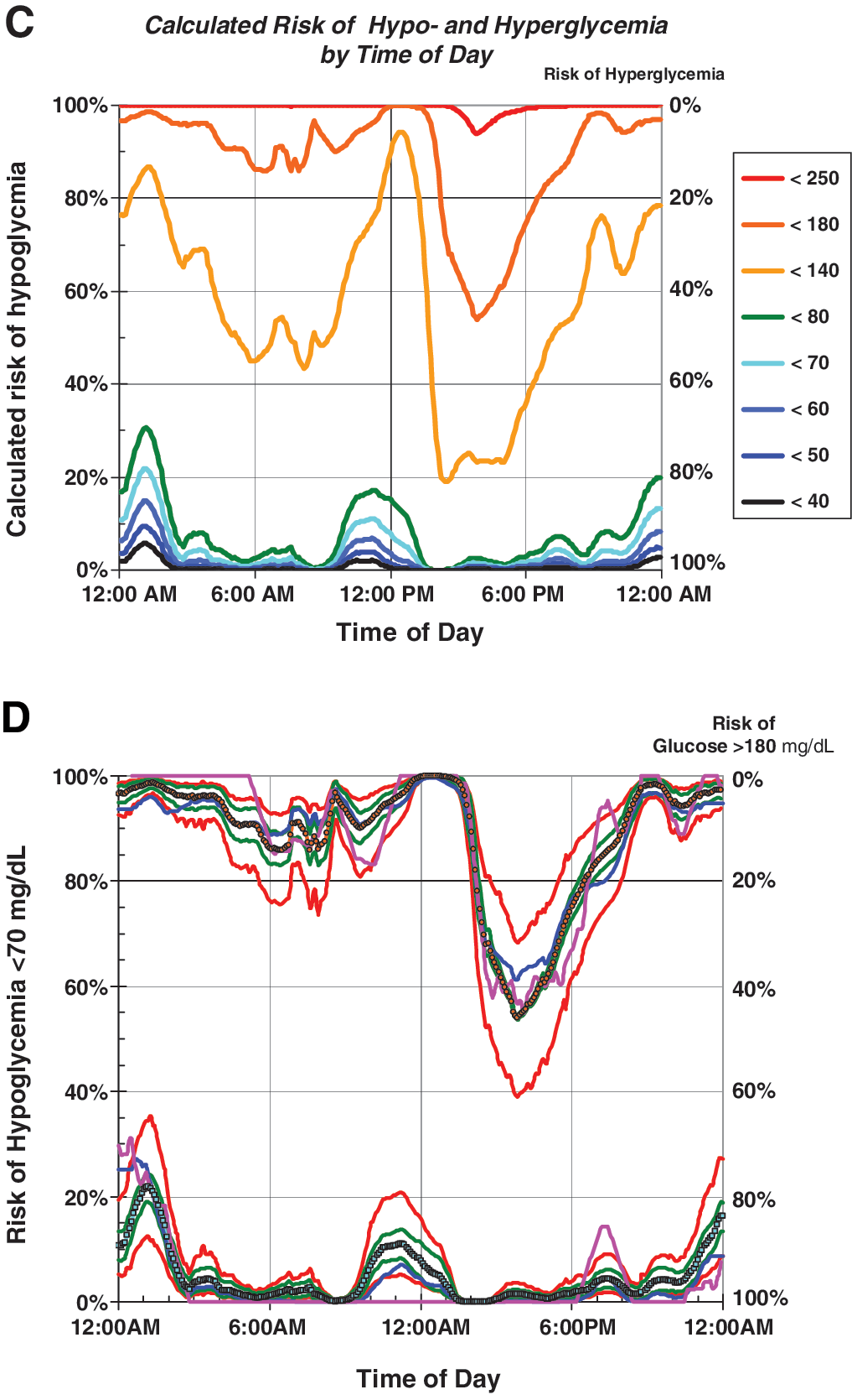
The calculation can be performed using just two instructions in Microsoft^® (Redmond, WA) Excel using Eqs. S1 and S2 (compare Supplementary Data, Appendix). Figure 2A and B shows the calculated probabilities of hypoglycemia and hyperglycemia, respectively, by time of day. One can calculate risks using any arbitrary threshold, including thresholds for which only a few events (or none at all) have been observed. Risks can also be displayed by date or day of the week. The risks of hypo- and hyperglycemia can be displayed simultaneously in one compact graph (Fig. 2C) by inverting the curves for hyperglycemia: rather than showing the expected percentage of glucose values above a given threshold (e.g., glucose >180 mg/dL) (Fig. 2B), one can show the expected percentage of values below the same threshold (glucose<180 mg/dL). This method of display (Fig. 2C) is closely related to the “stacked bar chart” for display of the observed percentages of glucose values within a specified series of ranges of glucose.^18,19

One can use several methods to evaluate the stability, robustness, and accuracy of the proposed method for estimating risk of hypo- and hyperglycemia. First, one can display the best estimates of the risks of hypo- and hyperglycemia graphically versus a variable of interest (e.g., time of day) as obtained using the present method and as observed empirically by counting “events” (Fig. 2D). Second, one can assess the effect of uncertainty in the mean glucose by showing the corresponding risks calculated on the basis of the (Mean+1 SEM) and the (Mean−1 SEM). Similarly, we can assess the magnitude of error likely to be introduced by random sampling error in the SD, using [ s +1 SE( s )] and [ s −1 SE( s )], where SE( s ) is the expected SE of the sample SD, calculated using available formulas.⁸ Figure 2D shows one example of the effects of those types of uncertainties on the estimated patterns for risk of hypo- and hyperglycemia. Finally, one can examine the effects of the choice of transformation to achieve a Gaussian distribution. One can address this by considering two of the extreme cases: use of c=0, which corresponds to a simple log transform, and c=“infinity,” which is mathematically equivalent to assuming that the original glucose values have a Gaussian distribution. If these two extremes produce similar results, then the results can be deemed to be largely independent of the choice of transformation. In the present example, similar results were obtained with or without the use of the log transform applied to the glucose data (Fig. 2D).

Analysis of a patient population

Utilizing data from 81 subjects using masked CGM for a period of 1 week¹⁷ where the mean, SD, and observed rates of hypo- and hyperglycemia were available for each subject, we compared the predicted probabilities with the observed number of events for hypo- and hyperglycemia using multiple specified thresholds (Fig. 3). The correlation of predicted and observed rates for hyperglycemia at 180 and 250 mg were particularly good (both r=0.98). The correlation of observed and predicted rates for hypoglycemia at 80 mg/dL was fair (r=0.86), but the correlation using a threshold of 50 mg/dL was lower (r=0.65), in part because of a nearly 10-fold smaller number of observed events. These calculations were performed assuming that the original glucose distributions were Gaussian without transformation of the glucose scale. Better correlations might have been obtained if one were to optimize the symmetry of the distributions using transformations such as Eqs. 1 and 2 above.

FIG. 3.

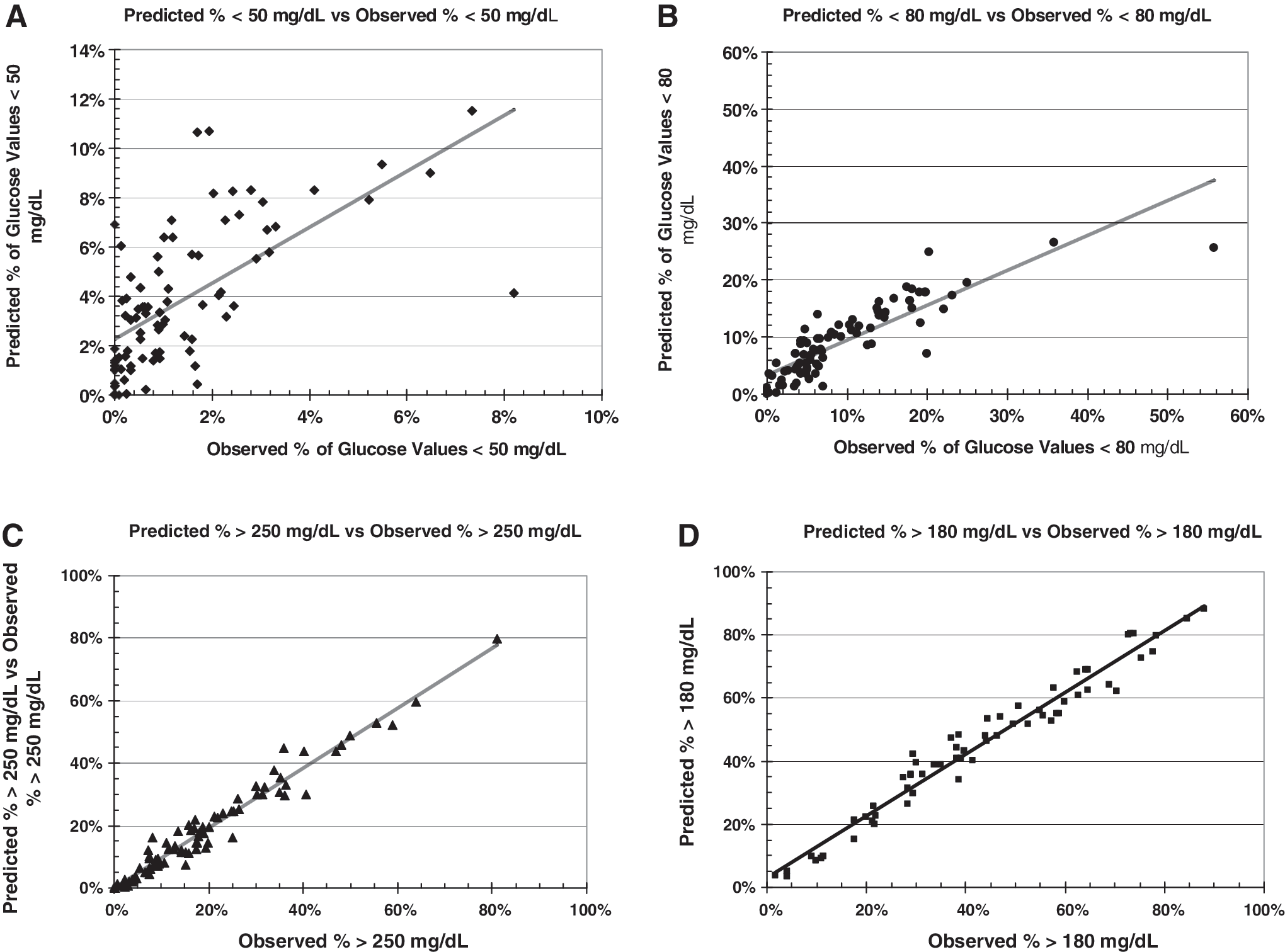
Correlation of calculated risks of hypo- and hyperglycemia assuming a Gaussian distribution (without transformation) (vertical axis) and observed risks (horizontal axis) based on observed events. Data are from Rodbard et al.¹⁷ for 81 subjects (64 with type 1 diabetes, 17 with type 2 diabetes, all receiving basal-bolus therapy with continuous subcutaneous insulin infusion or multiple daily injections, studied for 1 week with masked continuous glucose monitoring). Thresholds were (A) 50 mg/dL (r=0.65), (B) 80 mg/dL (r=0.86), (C) 250 mg/dL (r=0.98), and (D) 180 mg/dL (r=0.98). The correlation shown in Fig. 3B using the present proposed method using a Gaussian model (r=0.86) was superior to the correlation using several empirical models, for example, using simple linear regression versus percentage coefficient of variation (r=0.53), multiple regression of percentage of glucose values <80 mg/dL versus Mean and s (r=0.54), or multiple regression versus Mean and percentage coefficient of variation (r=0.58), or versus log(Mean) and log( s ) (r=0.59).

Potential use of surrogate markers for hypo- and hyperglycemia: correlation of risks of hypoglycemia at two thresholds (80 and 50 mg/dL) and of risks of hyperglycemia at two thresholds (180 and 250 mg/dL)

Figure 4A examines the relationship between the observed rates of hypoglycemia using two thresholds: <50 and <80 mg/dL. Figure 4B displays the relationship of observed rates of hyperglycemia using two thresholds: >180 and >250 mg/dL. There is a high correlation in both cases, confirming that the higher threshold (80 mg/dL) might be suitable for use as a proxy to estimate the risk of more severe hypoglycemia (50 mg/dL). The risk of events below 80 mg/dL can be measured much more accurately than the risk of events <50 mg/dL because of the much larger number of events when using the higher threshold (<80 mg/dL). Similarly, the risk of hyperglycemia using a threshold of >180 mg/dL can be regarded as a proxy for the risks of events at higher levels (e.g., >250, >300, or >400 mg/dL).

FIG. 4.

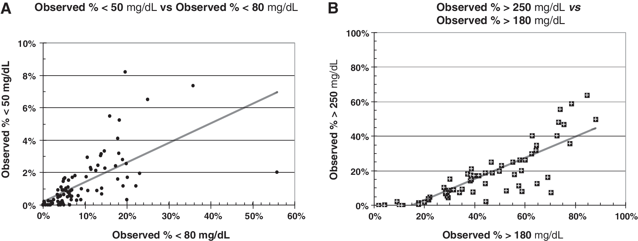
Use of surrogate markers for more severe levels of hypo- and hyperglycemia. Data are from Rodbard et al.¹⁷ for 81 subjects (64 with type 1 diabetes, 17 with type 2 diabetes, all receiving basal-bolus therapy with continuous subcutaneous insulin infusion or multiple daily injections, studied for 1 week with masked continuous glucose monitoring). (A) Correlation of observed frequency of events with glucose <50 mg/dL with observed frequency of events with glucose <80 mg/dL (r=0.64). Note the sixfold difference of numerical scales. (B) Correlation of observed frequency of events when glucose >250 mg/dL with observed frequency of events when glucose >180 mg/dL (r=0.84).

Correlation of risk of hypoglycemia and %CV for glucose

Figure 5 shows the relationship between risk of hypoglycemia in the same 81 subjects (data of Rodbard et al.¹⁷) versus the %CV for glucose (%CV=100 s /Mean), utilizing the Mean, s, and observed frequency of hypoglycemia for each subject. Highly significant correlations were obtained, consistent with previous findings.^3
–5

FIG. 5.

Relationships between percentage coefficient of variation (%CV) and risk of hypoglycemia using thresholds of glucose <80 mg/dL (black solid diamonds and black solid line) and <50 mg/dL (blue open circles and blue dashed line), for data for 81 subjects studied for 1 week using masked continuous glucose monitoring.¹⁷ Highly significant correlations were observed (r=0.53 for a threshold of <80 mg/dL; r=0.49 for a threshold of 50 mg/dL).

Conclusions

The present study demonstrates that one can obtain reasonably reliable estimates of the historical risks of hypo- or hyperglycemia for any desired arbitrary glucose threshold by transforming glucose values to achieve a (nearly) Gaussian distribution. If we assume that the patient's pattern remains stable over time, then one can use retrospective data to predict future risks by time of day (Fig. 2) or day of the week for individuals and groups of subjects. The results can be insensitive to the choice of transformation for the glucose values, indicating robustness of the method (Fig. 2D). The present method can be used to estimate the risk of rare events (e.g., severe hypoglycemia), even when such events have not been observed.

There was excellent agreement between observed and calculated risks of hypo- and hyperglycemia using a large dataset, assuming a Gaussian glucose distribution for each subject (Fig. 3), with thresholds of 50, 80, 180, and 250 mg/dL. Even better correlations might have been obtained with use of nonlinear transformations of the glucose scale.

Surrogate markers for hypoglycemia

In view of the relative infrequency of severe hypoglycemic events (e.g., <50 mg/dL or lower thresholds), Rodbard et al.²⁰ suggested that there was a need for surrogate markers and further suggested that the frequency of glucose values below 100 mg/dL might be a useful surrogate for clinically significant hypoglycemia at lower thresholds (e.g., <70 or <50 mg/dL). The calculated patterns of risk for hypoglycemia often have a very similar shape for a wide range of thresholds (e.g., 40–80 mg/dL) (Fig. 2A). Figure 3 confirms these relationships between risks calculated with different thresholds, using data from masked CGM of 1-week duration,¹⁷ where each data point represents a different study participant. These results support the use of the much larger (and thus more accurately and precisely measured) risks of glucose below 80 mg/dL as an effective surrogate marker to predict the risks of more severe hypoglycemia (e.g., for evaluation of the relative risk of hypoglycemia associated with different forms of therapy).²⁰

It would be desirable to conduct larger-scale studies to assess the performance of this approach applied to both CGM and self-monitoring of blood glucose specifically to examine the effects of differing categories of patients, differing types of treatments, differing amounts of data for each subject, and differing types of glucose distributions. The computational methods required are simple and can be readily implemented utilizing spreadsheets. However, it would be desirable to have these methods incorporated into fully automated software to reduce the risk of user errors. Furthermore, it would be desirable to compare the performance of the method proposed here with alternative methods for prediction of hypo- and hyperglycemia such as Low Blood Glucose Index,² High Blood Glucose Index, Hypoglycemia Index, Hyperglycemia Index,^15,16 GRADE_Hypoglycemia, GRADE_{Hyperglycemia},²¹ and %CV.

The present analysis emphasizes the critical importance of glycemic variability in determining the risks of hypo- and hyperglycemia and makes it possible to predict the relationships of the Mean, SD, and %CV of glucose to those risks. The Supplementary Data illustrate the interaction of the Mean and SD in determining the risks of hypo- or hyperglycemia. If there is a low Mean glucose and a large SD and hence a large %CV, the risk of hypoglycemia will be high. In contrast, if both the Mean and SD are high but with a low %CV, the risk of hypoglycemia will be relatively low. Similar kinds of statements can be made for the risk of hyperglycemia: a high Mean will generate a high frequency of hyperglycemia that is relatively insensitive to the magnitude of the SD. A lower mean could generate a high risk of hyperglycemia if the SD is large but not if the SD were small. These inferences can be demonstrated rigorously mathematically and follow directly from Eqs. S1 and S2 (cf. Supplementary Data). These calculations can be performed for any specified shape of the glucose distribution.

We have recently proposed²² that the %CV may be the best parameter to use to characterize glycemic variability in view of the relative constancy of its percentiles irrespective of glycated hemoglobin or mean glucose levels, which avoids the strong dependency of SD and other measures on mean glucose level or glycated hemoglobin. The correlation of %CV with risk of hypoglycemia has been observed empirically (Fig. 5) in the present study, and by others.^3
–5,23 This relationship can be predicted theoretically irrespective of the glucose level chosen as the criterion for hypoglycemia (see Supplementary Fig. S1). These observations enhance the importance of %CV as a parameter to describe glycemic variability.

Footnotes

Author Disclosure Statement

The author has served as a consultant to the following: Amylin, DexCom, Halozyme, LifeScan, Merck, Roche Diagnostics, Sanofi, University of Colorado, and Walter Reed National Medical Center.

References

Kovatchev

, Cox

, Gonder-Frederick

, Clarke

. Symmetrization of the blood glucose measurement scale and its applications. Diabetes Care, 1997; 20:1655–1658.

Kovatchev

, Cox

, Gonder-Frederick

, Young-Hyman

, Schlundt

, Clarke

. Assessment of risk for severe hypoglycemia among adults with IDDM: validation of the Low Blood Glucose Index. Diabetes Care, 1998; 21:1870–1875.

Monnier

, Wojtusciszyn

, Colette

, Owens

. The contribution of glucose variability to asymptomatic hypoglycemia in persons with type 2 diabetes. Diabetes Technol Ther, 2011; 13:813–818.

, Jacober

, Zhang

, Wolka

, DeVries

. The effect of glucose variability on the rate of hypoglycemic events [abstract 479-P] Diabetes, 2011; 60,Suppl 1:A133.

Inzucchi

, Umpierrez

, DiGenio

, Zhou

, Kovatchev

. Association of measures of glycemic variability with glycemic control and hypoglycemic events [abstract] Diabetes, 2012; 61,Suppl 1:A291.

Swinnen

SGHA

, Mullins

, Miller

, Hoekstra

JBL

, Holleman

. Changing the glucose cut-off values that define hypoglycaemia has a major effect on reported frequencies of hypoglycaemia. Diabetologia, 2009; 52:38–41.

Rodbard

. Optimizing display, analysis, interpretation and utility of self-monitoring of blood glucose (SMBG) data for management of patients with diabetes. J Diabetes Sci Technol, 2007; 1:62–71.

Ahn

, Fessler

. Standard Errors of Mean, Variance, Standard Deviation Estimators. www.eecs.umich.edu/∼fessler/papers/files/tr/stderr.pdf. 2012 February 2.

Rodbard

. Predicting the risk of hypo- and hyperglycemia by time of day, date, and day of the week—new methods for calculation and graphical display [abstract 491-P] Diabetes, 2010; 59,Suppl 1:A132.

10.

Shapiro

, Wilk

. An analysis of variance test for normality (complete samples) Biometrika, 1965; 52:591–611.

11.

Abramowitz

, Stegeun

. National Institute of Science and Technology: Engineering Statistics Handbook. 1.3.3.24. NIST/SEMATECH e-Handbook of Statistical Methods. www.itl.nist.gov/div898/handbook/eda/section3/qqplot.htm. 2012 July 23.

12.

Wikipedia: Q-Q Plot. http://en.wikipedia.org/wiki/Q%E2%80%93Q_plot. 2012 August 16.

13.

Finney

. Probit Analysis, 3 ^rd. Cambridge, UK: Cambridge University Press, 1971. http://en.wikipedia.org/wiki/International_Standard_Book_Number. 2012 July 23.

14.

Abramowitz

, Stegun

. Handbook of Mathematical Functions with Formulas Graphs, Mathematical Tables. New York: Dover, 1965; 297. www.math.sfu.ca/∼cbm/aands/page_297.htm. 2012 July 23.

15.

Rodbard

. Interpretation of continuous glucose monitoring data: glycemic variability, quality of glycemic control. Diabetes Technol Ther, 2009; 11,Suppl 1:S-55–S-57.

16.

Rodbard

. New and improved methods to characterize glycemic variability using continuous glucose monitoring. Diabetes Technol Ther, 2009; 11:551–565.

17.

Rodbard

, Bailey

, Jovanovic

, Zisser

, Kaplan

, Garg

. Improved quality of glycemic control and reduced glycemic variability with use of continuous glucose monitoring. Diabetes Technol Ther, 2009; 11:717–723.

18.

Levetan

, Want

, Weyer

, Strobel

, Crean

, Wang

, Maggs

, Kolterman

, Chandran

, Mudaliar

, Henry

. Impact of pramlintide on glucose fluctuations and postprandial glucose, glucagon, and triglyceride excursions among patients with type 1 diabetes intensively treated with insulin pumps. Diabetes Care, 2003; 26:1–8.

19.

Rodbard

. Display of glucose distributions by date, time of day, and day of week: new and improved methods. J Diabetes Sci Technol, 2009; 3:1388–1394.

20.

Rodbard

, Berger

, Pernick

. Computer, networking, and information systems to facilitate delivery of health care to patients with diabetes. Baba

, Kaneko

. Diabetes 1994, Proceedings of the 15th International Diabetes Federation Congress, Kobe, November 6–11, 1994. Amsterdam: Elsevier, 1995; 800–803.

21.

Hill

, Hindmarsh

, Stevens

, Stratton

, Levy

, Matthews

. A method for assessing quality of control from glucose profiles. Diabet Med, 2007; 24:753–758.

22.

Rodbard

. Clinical interpretation of indices of quality of glycemic control and glycemic variability. Postgrad Med, 2011; 123:107–118.

23.

, Jacober

, Zhang

, Wolka

, DeVries

. Rate of hypoglycemia in insulin-treated patients with type 2 diabetes can be predicted from glycemic variability data. Diabetes Technol Ther, 2012in press.

Supplementary Material

Please find the following supplemental material available below.

For Open Access articles published under a Creative Commons License, all supplemental material carries the same license as the article it is associated with.

For non-Open Access articles published, all supplemental material carries a non-exclusive license, and permission requests for re-use of supplemental material or any part of supplemental material shall be sent directly to the copyright owner as specified in the copyright notice associated with the article.

0.00 MB

0.13 MB

Hypo- and Hyperglycemia in Relation to the Mean,Standard Deviation,Coefficient of Variation,and Nature of the Glucose Distribution

Abstract

Aims:

Materials and Methods:

Results:

Conclusions:

Introduction

Principle of the present method

Materials and Methods

Box 1. Simplified Schematic of the Proposed Method to Estimate the Probabilities of Hypo- or Hyperglycemia Using Any Desired Threshold

Results

Estimation of the risk of hypo- and hyperglycemia based on a Gaussian distribution for glucose (G) or a transformed glucose value (G ′)

Analysis of a patient population

Potential use of surrogate markers for hypo- and hyperglycemia: correlation of risks of hypoglycemia at two thresholds (80 and 50 mg/dL) and of risks of hyperglycemia at two thresholds (180 and 250 mg/dL)

Correlation of risk of hypoglycemia and %CV for glucose

Conclusions

Surrogate markers for hypoglycemia

Footnotes

Author Disclosure Statement

References

Supplementary Material

Estimation of the risk of hypo- and hyperglycemia based on a Gaussian distribution for glucose (G) or a transformed glucose value (G ^′)