Mathematical Modeling of the Transmission and Control of Foodborne Pathogens and Antimicrobial Resistance at Preharvest

Abstract

Foodborne diseases are a significant health-care and economic burden. Most foodborne pathogens are enteric pathogens harbored in the gastrointestinal tract of farm animals. Understanding the transmission of foodborne pathogens and the dissemination of antimicrobial resistance at the farm level is necessary to design effective control strategies at preharvest. Mathematical models improve our understanding of pathogen dynamics by providing a theoretical framework in which factors affecting transmission and control of the pathogens can be explicitly considered. In this review, we aim to present the principles underlying the mathematical modeling of foodborne pathogens and antimicrobial resistance at the farm level to a broader audience.

Introduction

F oodborne diseases are a significant health-care and economic burden. In 2008, the CDC's Foodborne Diseases Active Surveillance Network (FoodNet) estimated that the incidence of illnesses caused by foodborne pathogens in the United States had not decreased since 2004 as far as Campylobacter, Listeria, Escherichia coli O157, Salmonella, Shigella, Vibrio, and Yersinia infections were concerned, whereas Cryptosporidium infections increased by 44% (CDC, 2008). Most of these foodborne pathogens are enteric pathogens that are harbored in the gastrointestinal tract of farm animals and found in their associated farm environments (Oliver et al., 2009). Antimicrobial resistance is also considered a food safety issue because infections with multidrug-resistant (MDR) foodborne pathogens can be particularly serious. For example, patients infected with MDR Salmonella strains are at greater risk of bacteremia, hospitalization, and death than patients infected with susceptible strains (Varma et al., 2005). Although the dissemination of antimicrobial resistance among commensal enteric bacteria is poorly understood, it has been postulated that the food supply may be a source of antimicrobial resistance genes as commensal bacteria can harbor resistance genes that can be potentially transferred to pathogenic bacteria (Levy and Marshall, 2004). Emergence and dissemination of antimicrobial resistance have proved to be ubiquitous processes; reservoirs of resistance genes have been described in several environments, including commensal bacteria in human and animal gastrointestinal tracts (Salyers et al., 2004).

Understanding the transmission of foodborne pathogens and dissemination of antimicrobial resistance at the farm level is necessary to design effective control strategies. Advances in microbiological methods and epidemiological research have significantly progressed our understanding of foodborne diseases and the impact of implementing control programs at preharvest (Torrence, 2005). Epidemiological studies have measured the prevalence of foodborne pathogens at the farm level and studied the association between carriage of foodborne pathogens and animal and herd level variables using risk factor analysis (Fossler et al., 2005a, 2005b). Molecular epidemiology has unraveled the complex dynamics underlying zoonotic enteric pathogen presence at the farm level. It has aided the identification of both host and environmental reservoirs and provided evidence of multiple introductions and transmission (Weigel et al., 2007). Further elucidation of effective control strategies requires methods that are able to explicitly consider transmission pathways and the ecology of the zoonotic enteric pathogens at the farm level. In recent years, mathematical models of infection transmission have been incorporated in the epidemiologist repertoire. Mathematical models provide a conceptual framework for understanding pathogen ecology and quantifying the effects of intervention strategies (Anderson and May, 1992). Mathematical models have been used (1) to interpret and identify processes underlying epidemiological data, (2) to identify knowledge gaps and guide new data collection, and (3) to identify, design and optimize control interventions. In this article, we introduce the principles underlying the mathematical models used to understand foodborne pathogens transmission and to design and evaluate control strategies at the farm level. The review is organized as follows. In the Introduction to Mathematical Modeling section, we introduce the basic steps in modeling and refer the reader to further sources of modeling information. In the following four sections, we review the key common aspects underlying the transmission dynamics of foodborne pathogens at the farm level. We discuss how different sources of variation that affect transmission and control strategies can be included and studied using epidemiological models. Finally, we address the use of mathematical models to study antimicrobial resistance.

Introduction to Mathematical Modeling

Mathematical modeling is the process of constructing, testing, and improving mathematical models, which are representations of systems or hypotheses in a mathematical language. The steps in mathematical modeling parallel those of the scientific method. We formulate the research question, develop the mathematical model, analyze and validate the mathematical model, and, finally, relate the model back to the research question (Otto and Day, 2007). The research question or intended use of the model is one of the most important aspects guiding the development of the models because the model structure needs to be adequate to address our objectives. The need to understand the mechanisms that cause the patterns present in observed data is often the objective that initiates the modeling process.

The existent literature in mathematical modeling is very extensive. Here we review its application in studying foodborne pathogens. We refer the reader to several books that provide a more general overview of mathematical modeling and its use in infectious disease modeling. Otto and Day (2007) provide a comprehensive review of the different mathematical methods used in biological modeling. Anderson and May (1992) and Keeling and Rohani (2008) provide an overview of the use of mathematical models in infectious disease epidemiology.

Transmission of Foodborne Pathogens at the Farm Level

While each foodborne pathogen has its own population dynamics and specific interactions with their hosts, there are common aspects underlying their transmission at the farm level. Most of the foodborne pathogens live in the gastrointestinal tract of animals; therefore, fecal shedding is the main route of pathogen excretion. There is large variation in the pathogen shedding level among animals, as well as fluctuations in the level shed by a single animal. For example, counts of E. coli O157:H7 in cattle feces ranged from 1 CFU to 1.6 × 10⁶ CFU/g of feces; this variation was attributed mostly to within-animal differences in the shedding level over time (Robinson et al., 2009). In addition, foodborne pathogens often behave as commensals in the animal reservoirs, and therefore the animals are asymptomatically colonized. Foodborne pathogens can often survive and even grow in the farm environment (e.g., in water troughs and feedbunks) and in animal reservoirs other than farm animals (e.g., in pest and wildlife animals) (Lejeune et al., 2001; Oliver et al., 2007). As a consequence, there are multiple direct (e.g., fecal–oral and oral–oral) and indirect (e.g., through environment or mechanical vectors) routes of transmission.

A conceptual model for foodborne pathogens transmission that incorporates some of the above aspects is presented in Figure 1. The most widely used mathematical models for infectious diseases are the so-called susceptible-infectious-recovered (SIR) compartmental models. In SIR models, the host population is divided into compartments according to its epidemiological status (e.g., susceptible, infectious, and recovered). Susceptible animals are those not infected, but which may become infected later. Infectious animals are infected animals that shed the pathogen and, therefore, can infect other animals. Recovered animals have immunity against the pathogen. Immunity lasts for a limited period after which animals become susceptible again. Infection with the pathogen can result in clinical disease or subclinical carriage, and thus we consider two types of infectious animals: clinically infectious (I _c) and subclinically infectious (I _s) animals (Fig. 1). Infectious animals shed the pathogen into the environment (W). 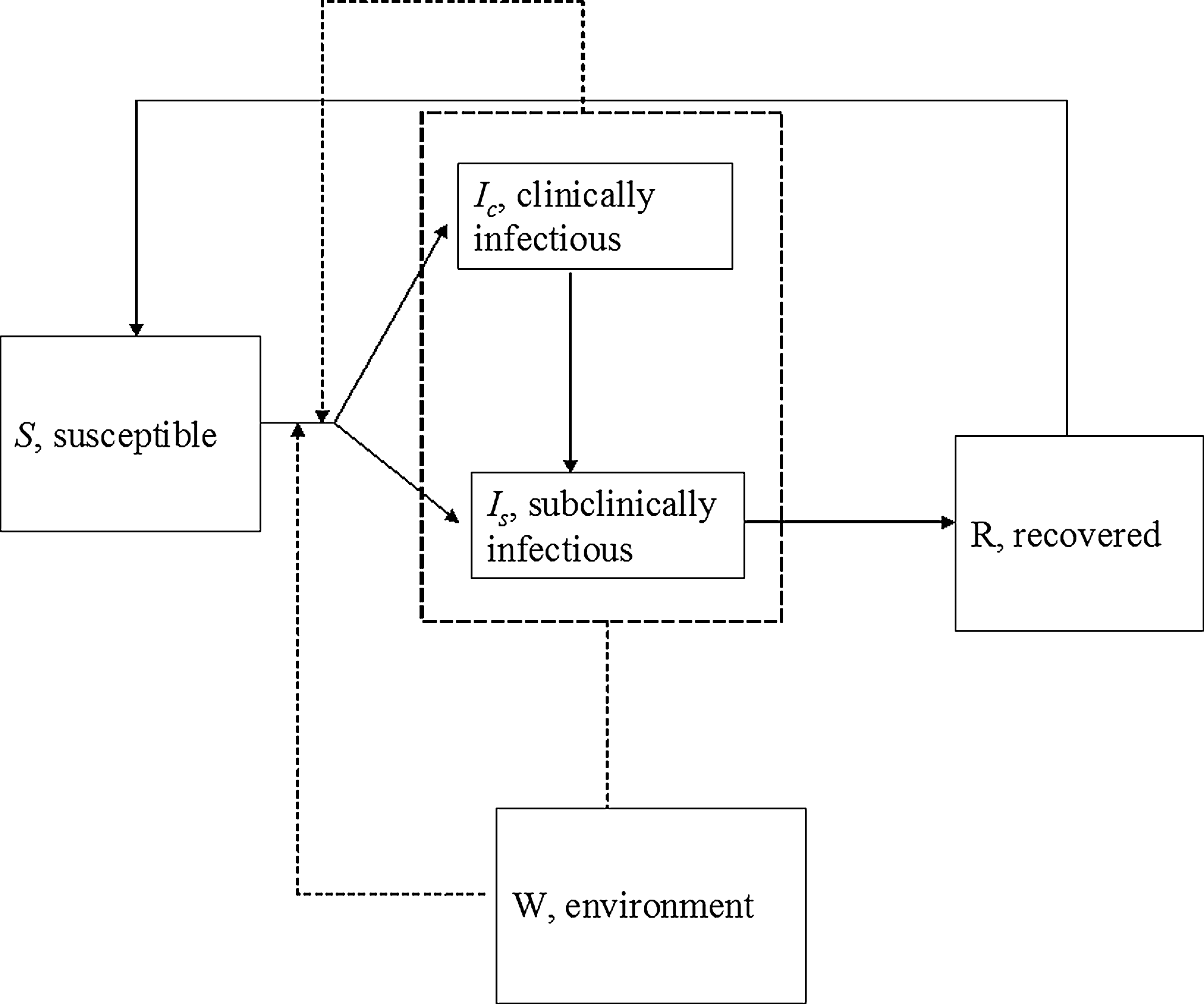The Supplemental Material (available online at www.liebertonline.com) describes the differential equations that define the state transition model in Figure 1. The differential equations describe the change over time in the number of animals in each compartment.

FIG. 1.

Conceptual model for foodborne pathogens transmission within animal populations. Transition states for the animals include S (susceptible), I _c (clinically infectious), I _s (subclinically infectious), and R (recovered). Pathogens are shed to the environment, W. Transmission takes place directly, through contact with infectious animals, or indirectly, through the contact with the free-living pathogen in the environment. Solid arrows indicate movement of animals through the different transition states. Dashed arrows indicate sources of new infections.

Not all the transition states in Figure 1 are applicable for all foodborne pathogens. The choice of which transition states to include in a model depends on the host–pathogen being modeled and the purpose of the model. Table 1 shows the epidemiological compartments commonly considered for some foodborne pathogens. For bacteria that behave as commensals (e.g., Campylobacter jejuni in poultry), the susceptible and infectious states are often the only epidemiological states considered in the model. Differences in infectiousness because of different levels of pathogen shedding can be accounted for by including two infectious states, high and low level shedders. A carrier status may be included to describe those animals carrying the pathogen, but not shedding it (Lurette et al., 2008). In addition to their epidemiological status, animals can be classified in age or group classes if there are differences in risk of acquiring and spreading the foodborne pathogen (discussed in the next section).

Table 1.

Most Common Epidemiological Status Considered for Some Foodborne Pathogens Found in Farm Animals

Pathogen	Animal reservoirs	Epidemiological status
Campylobacter spp.	Poultry, cattle, swine	S, I
Escherichia coli O157:H7	Cattle	S, I
Mycobacterium ^a	Cattle	S, I _t, I _l, I _ls, I _hs
Salmonella nontyphoidal	Poultry, cattle, swine	S, I _c, I _s, C, R
Yersinia enterocolitica	Swine	S, I, C

While Mycobacterium avium subsp. paratuberculosis (MAP) has not been definitively shown to be a zoonotic agent, there are a number of studies linking MAP to Crohn's disease, a chronic intestinal disease in humans (Collins, 1997).

S, susceptible; C, carrier; I, infectious; I _t, infectious transient shedder; I _l, latent infectious; I _ls, infectious low shedder; I _hs, infectious high shedder; I _c, clinically infectious; I _s, subclinically infectious; R, recovered.

Transmission is the key process underlying infectious disease models. The transmission term of an epidemiological model describes how animals acquire the pathogen. For a pathogen that is transmitted directly from animal to animal, its transmission depends on the prevalence of infectious animals (I/N, where I = infectious and N = total population), the population contact structure, and the probability of transmission given contact between a susceptible and an infectious animal (Keeling and Rohani, 2008). If the rate of contact increases directly with the population size, transmission is said to be “density dependent,” whereas if the rate of contact does not increase with population size, transmission is “frequency dependent” (Keeling and Rohani, 2008). Susceptible animals may get infected upon contact with an infectious individual (i.e., direct contact) or with free-living bacteria present in the environment (i.e., indirect contact). The transmission term for the model in Figure 1 is density dependent (Keeling and Rohani, 2008) and includes both direct and indirect transmission pathways and is described as follows, \documentclass{aastex}\usepackage{amsbsy}\usepackage{amsfonts}\usepackage{amssymb}\usepackage{bm}\usepackage{mathrsfs}\usepackage{pifont}\usepackage{stmaryrd}\usepackage{textcomp}\usepackage{portland, xspace}\usepackage{amsmath, amsxtra}\pagestyle{empty}\DeclareMathSizes{10}{9}{7}{6}\begin{document}\begin{align*}(\beta_{c}I_{c} + \beta_{s}I_{s} + \pi \eta W) S \tag{1}\end{align*}\end{document}

where β _c and β _s are the transmission coefficients for clinically and subclinically infectious animals (animal⁻¹ day⁻¹). The term βI is the per capita rate of transmission (day⁻¹) and captures the product of the rate of contact between individuals, the probability that the contact is with an infectious individual, and the probability that the contact with an infectious individual leads to infection as explained above (Begon et al., 2002). The indirect transmission is represented by the term πηW, where W is the environmental compartment representing the free-living bacteria in the environment, η is the contact rate between animals and free-living bacteria, and π is the probability of infection from contact with free-living bacteria. Another important parameter in infectious disease models is the recovery rate. The recovery rate is the rate at which individuals leave the infectious compartment and equals the inverse of the infectious period. The infectious period is the time period during which an infectious individual sheds the pathogen; for pathogens that transmit through oral–fecal route, the duration of fecal shedding is used as an estimate of the infectious period (Lanzas et al., 2008a).

To evaluate whether the pathogen would propagate within a population or not, the basic reproduction number (R ₀) is often estimated using mathematical models (Heffernan et al., 2005). The basic reproduction number is the expected number of secondary cases produced by a typical infected individual during its infectious period in a completely susceptible population (Anderson and May, 1992). For a SIR model with one category of infectious individuals and direct contact transmission, R ₀ is the product of the transmission rate and the mean duration of the infectious period. The basic reproduction number is a threshold quantity because if R ₀ is greater than one, on average one case leads to more than one secondary case, and therefore the number of cases will grow in the population. If R ₀ is less than one, on average one case leads to less than one secondary case, and the infection will die out in the population. The greater the R ₀, the greater are the efforts necessary to control the pathogen in the population. The basic reproduction number has been estimated for some foodborne pathogens; for E. coli O157, R ₀ has been estimated to be 4.3 in beef cattle populations (Laegreid and Keen, 2004), 1.3–5.8 for Salmonella in dairy cow populations (Van Schaik et al., 2007; Chapagain et al., 2008), and 2.8 for Salmonella in laying hens populations (Thomas et al., 2009).

Indirect transmission of foodborne pathogens can also take place through contaminated fomites and mechanical vectors. With individually penned animals, this cross-infection (indirect transmission) between infected animals and contaminated fomites and vectors represents an important route of transmission (Hardman et al., 1991). The SIR model framework used for vector-borne diseases such as malaria (Anderson and May, 1992) can be adopted to make the role that personnel and equipment play in the transmission of foodborne pathogens more explicit. Lanzas et al. (2008b) developed an indirect transmission model to address Salmonella transmission in a calf-raising operation. In the model, calves (host population) contaminated the workers/equipment (defined in the model as vector population), and contaminated vectors then infected calves, completing the transmission cycle (Fig. 2). For this model, the basic reproduction number is \documentclass{aastex}\usepackage{amsbsy}\usepackage{amsfonts}\usepackage{amssymb}\usepackage{bm}\usepackage{mathrsfs}\usepackage{pifont}\usepackage{stmaryrd}\usepackage{textcomp}\usepackage{portland, xspace}\usepackage{amsmath, amsxtra}\pagestyle{empty}\DeclareMathSizes{10}{9}{7}{6}\begin{document}\begin{align*}R_{0} = \sqrt \frac {c^ {2} p_{i} p_{c}}{(m + \gamma) \alpha} \tag {2} \end{align*}\end{document}

FIG. 2.

Indirect transmission model flow chart (adapted from Lanzas et al., 2008b). Individuals (host population) contaminated the workers/equipment (vector population), and contaminated vectors then infected individuals completing the transmission cycle. The transition states for the animals are susceptible (S), infectious (I), and recovered (R). The transition states for the vector population are free (V ⁻) or contaminated (V ⁺) with the pathogen. Solid arrows indicate movement of individuals and workers through the different transition states. Animals can enter and exit the facility in any of the three states. Dashed arrows indicate sources of new infection and contamination.

where α is the decontamination rate (day⁻¹), c is the contact rate per animal per vector (day⁻¹), γ is the recovery rate (day⁻¹), m is the pathogen-induced mortality rate (day⁻¹), p _i is the proportion of contacts between contaminated vectors and susceptible animals leading to animal infection, and p _c is the proportion of contacts between infected animals and uncontaminated vectors leading to contaminated vectors. The basic reproduction number was estimated to be 2.4 (Lanzas et al., 2008b). In this model, R ₀ is a function of the squared contact rate (see Equation 3) because two contacts are necessary for animal to animal transmission. Therefore, decreasing the contact between fomites and animals (e.g., use of separate set of clothing and boots for different animal groups) is an effective way of reducing R ₀.

Sources of Heterogeneity in the Transmission of Foodborne Pathogens at the Farm Level

The contribution of different infectious individuals to the R ₀ can vary because differences in contacts, transmission routes, or pathogen shedding among individuals results in different infectious individuals producing different numbers of secondary cases. The infectiousness of an individual may vary because differences in host–pathogen interactions and host characteristics such as vaccination status, age, and stress levels may result in different levels of pathogen excretion and duration of shedding. An important implication of the presence of infectious individuals contributing differently to new cases is that individual-specific control measures designed to target the most infectious individuals (e.g., isolation and culling) may be more efficient at controlling pathogen transmission than are population-wide control measures (e.g., vaccination at random) (Woolhouse et al., 1997; Lloyd-Smith et al., 2005b).

Mathematical models provide a framework to study the effect that different sources of heterogeneity have on transmission. In the models, the host population can be structured in distinct categories (e.g., different levels of infectiousness or mixing patterns). The next-generation matrix method allows us to quantify the contribution of different infectious categories to new cases and express R ₀ as a function of model parameters for infectious disease models that include different host types and transmission routes (Diekmann and Heesterbeek, 2000; van den Driessche and Watmough, 2002). The Supplemental Material presents the derivation of the next-generation matrix (K) for the model in Figure 1. The entries in the matrix K are reproduction numbers for pair of types. Thus, the entries (i, j) of the next-generation matrix K have a clear biological meaning; it is the expected number of secondary infections in compartment i produced by individuals initially in compartment j. For example, the entry K _cc represents the contribution of individuals that were initially clinically infectious to new clinical cases. \documentclass{aastex}\usepackage{amsbsy}\usepackage{amsfonts}\usepackage{amssymb}\usepackage{bm}\usepackage{mathrsfs}\usepackage{pifont}\usepackage{stmaryrd}\usepackage{textcomp}\usepackage{portland, xspace}\usepackage{amsmath, amsxtra}\pagestyle{empty}\DeclareMathSizes{10}{9}{7}{6}\begin{document}\begin{align*}K_{cc} = \frac {f \beta_{c} S_{0}} {(e + \mu)} + \frac {ef \beta_{s} S_{0}} {(e + \mu) (h + \mu)} + \frac {f \pi \eta S_{0} [\lambda_{s} e + \lambda_{c} (h + \mu) ]} {(e + \mu) (h + \mu) \varphi} \tag {3} \end{align*}\end{document}

The first term, \documentclass{aastex}\usepackage{amsbsy}\usepackage{amsfonts}\usepackage{amssymb}\usepackage{bm}\usepackage{mathrsfs}\usepackage{pifont}\usepackage{stmaryrd}\usepackage{textcomp}\usepackage{portland, xspace}\usepackage{amsmath, amsxtra}\pagestyle{empty}\DeclareMathSizes{10}{9}{7}{6}\begin{document}$$\frac {f \beta_{c} S_{0}} {(e + \mu)}$$\end{document} , indicates the new clinical cases caused by a clinical case while remaining in the clinically infectious state, through direct transmission. The second term, \documentclass{aastex}\usepackage{amsbsy}\usepackage{amsfonts}\usepackage{amssymb}\usepackage{bm}\usepackage{mathrsfs}\usepackage{pifont}\usepackage{stmaryrd}\usepackage{textcomp}\usepackage{portland, xspace}\usepackage{amsmath, amsxtra}\pagestyle{empty}\DeclareMathSizes{10}{9}{7}{6}\begin{document}$$\frac {ef \beta_{s} S_{0}} {(e + \mu) (h + \mu)}$$\end{document} , indicates the new clinical cases caused by a clinical cause after clinical recovery, while it is subclinically infectious, through direct transmission. The third term, \documentclass{aastex}\usepackage{amsbsy}\usepackage{amsfonts}\usepackage{amssymb}\usepackage{bm}\usepackage{mathrsfs}\usepackage{pifont}\usepackage{stmaryrd}\usepackage{textcomp}\usepackage{portland, xspace}\usepackage{amsmath, amsxtra}\pagestyle{empty}\DeclareMathSizes{10}{9}{7}{6}\begin{document}$$\frac {f \pi \eta S_{0} [\lambda_{s} e + \lambda_{c} (h + \mu) ]} {(e + \mu) (h + \mu) \varphi}$$\end{document} , represents the contribution of the clinical case through indirect transmission (see Supplemental Material for parameter definitions).

Transmission of Salmonella in dairy herds is influenced by differences in contagiousness and duration of the infectious periods among infectious individuals. Lanzas et al. (2008a) developed three SIR-type models to address the contribution of four different types of infectious animals (clinically and subclinically infectious, long-term shedders, and super-shedders) to Salmonella transmission. Long-term shedders are animals that shed low bacteria counts for long periods. Super-shedders are animals that shed high bacteria counts. The next-generation matrix method was used to estimate the contribution of the four infectious types. The contribution of the long-term shedders (individuals with low contagiousness but long infectious periods) to the newly infected cases was 0.21 cases, suggesting that long-term shedders had a small impact on the transmission of the infection. The contribution of the super-shedders was 3.32 new cases. The presence of super-shedders increased R ₀ and decreased the effectiveness of population-wise strategies to reduce infection, making necessary the application of strategies that target this specific group (Lanzas et al., 2008a).

Group structure (e.g., pen and age divisions) causes differences in the mixing pattern of animals. Farm structure has been included in models for foodborne pathogens for dairy farms (Turner et al., 2003) and pig farms (Lurette et al., 2008). To model Salmonella spread in a farrow-to-finish pig farm, Lurette et al. (2008) explicitly modeled the batch farrowing management system and the mix of batches that can take place at the finishing stage. Models that incorporate group structure have shown that reducing the transmission between groups (controlling either indirect transmission or the movement of infectious animals) is necessary to reduce within herd prevalence (Turner et al., 2003).

Stochastic Transmission Dynamics

If an outbreak was to be repeated, we would not observe the same number of animals becoming infected at exactly the same times. Stochasticity (or randomness) causes fluctuations in the observed prevalence, and thus stochasticity needs to be taken into account when interpreting field data. We develop stochastic models to mimic the observed stochasticity in real observations. Transmission can be influenced by two sources of stochasticity (or variability), demographic and environmental stochasticity. Demographic stochasticity results from the probabilistic nature of individual processes such as birth, death, transmission, and recovery, and therefore it has a greater impact on small populations such as farms or when the number of infectious individuals is low (i.e., during the early phases of an outbreak or when the outbreak is dying out). The smaller the population, the greater the weight each individual carries in the population. Demographic stochasticity can be accounted for in the stochastic models by recasting the rates that appear in the deterministic models, whose predictions depend entirely on the model structure and initial values, in terms of probabilities. The stochastic model can then be simulated using event-driven methods (Gillespie, 1976). The event-driven simulation methods have been reviewed in Gillespie (2007). For the model depicted in Figure 1, the average subclinically and clinically infected animals predicted by the deterministic model and a stochastic realization of the model simulated using an event-driven method are presented in Figure 3. The stochastic realization depicts fluctuations in the number of infected animals. Simulating stochastic models is like performing an in silico experiment; a large number of simulations have to be undertaken to observe all the plausible trajectories.

FIG. 3.

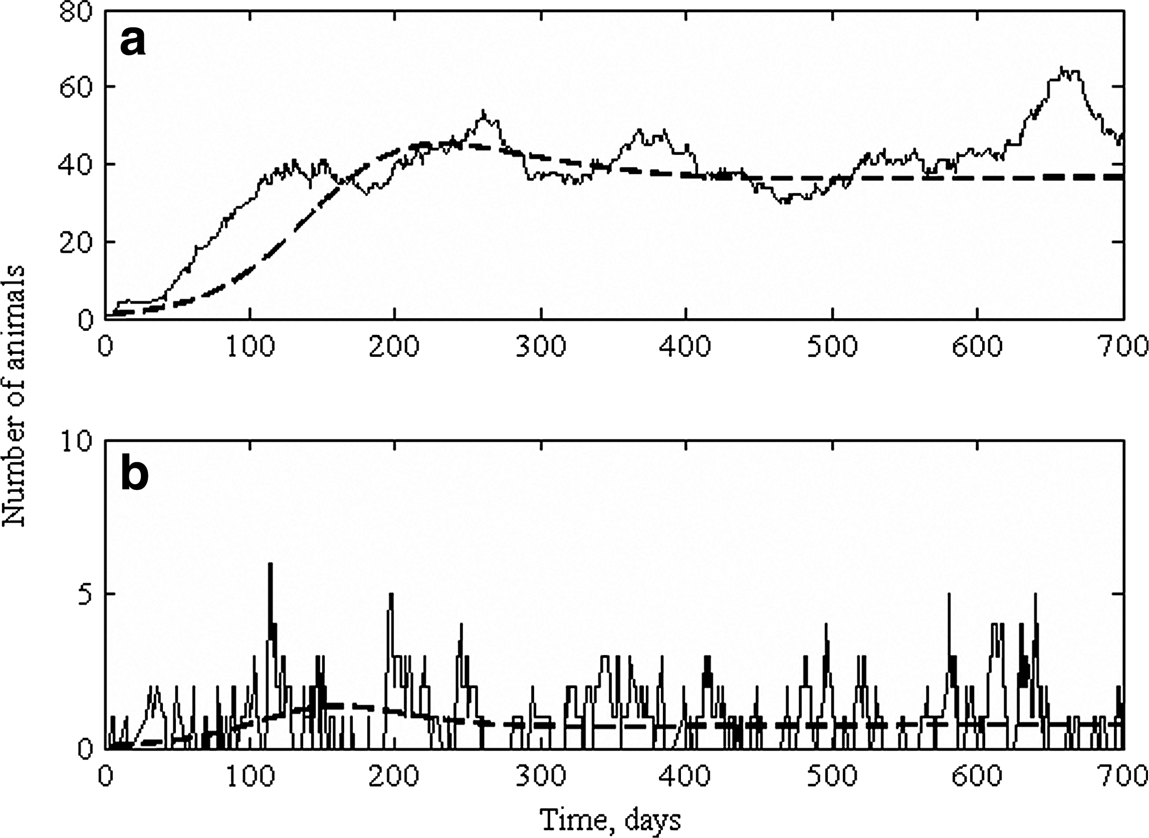
Simulated number of subclinically infectious individuals (a) and clinically infectious individuals (b) predicted by the deterministic version of the model depicted in Figure 1 (dashed lines). A stochastic realization illustrates the fluctuations that the demographic stochasticity causes in the number of infectious individuals (solid lines).

Demographic stochasticity, in addition to causing fluctuations in prevalence, increases the probability of breaking the chain of transmission (i.e., infectious animals fail to transmit to susceptible animals) and the probability that the pathogen goes extinct in the herd, with only a few infected animals as a final outbreak size. Stochastic models show us that a pathogen can fail to invade a population even when R ₀ > 1. Even with a large R ₀, “failure” outbreaks, also called fade-outs, can occur (Lloyd-Smith et al., 2005a). Small salmonellosis outbreaks are the most common presentation of MDR Salmonella infection in dairy herds (Cummings et al., 2009). Simulation studies indicated that the extinction of pathogens on the premises due to demographic stochasticity during the early phase of the outbreak was the most likely cause of the short-lived, small outbreaks (Lanzas et al., 2010). Similarly, demographic stochasticity may help to explain why herd size is often identified as a risk factor for foodborne pathogens shedding (Kabagambe et al., 2000) and salmonellosis (Cummings et al., 2009). The positive association between herd size and pathogen shedding has often been explained by management differences between large and small herds such as the higher tendency of a large operation to bring in new cattle (Kabagambe et al., 2000). However, demographic stochasticity and the scaling of transmission with population density if the transmission is density dependent can result in an increase in the persistence of the pathogen in larger herds, independent of management differences.

Environmental stochasticity arises from fluctuations in the environment (e.g., temperature and humidity can influence the survival of pathogens) and can influence seasonal foodborne pathogens shedding and prevalence trends (Stanford et al., 2005). Changes in temperatures can result in variation in the parameters related to the environmental compartment (e.g., ϕ, rate of removing free-living bacteria from the environment). In addition to seasonal changes in temperature, seasonality can have other causes. For example, moving animals from pasture to confinement (Ogden et al., 2004) can cause seasonal variation in the prevalence because the contact rate among animals changes, which subsequently affects transmission. This can be explored by including time-dependent transmission coefficients (β) in the models. Large and small populations are equally influenced by environmental stochasticity.

Control Strategies

Control strategies to reduce foodborne pathogen transmission can be classified as those strategies that aim to change management or to target the foodborne pathogen within the gastrointestinal tract. Management control strategies include test-and-cull intervention, improved hygiene, and isolation. Control strategies that target the foodborne pathogen at the gastrointestinal tract level include vaccination, probiotics, therapeutic treatments, and nutritional control strategies (Callaway et al., 2003). The effect of control strategies on foodborne pathogens transmission can be evaluated in mathematical models by predicting the R ₀, the duration and size of outbreaks, or the change in prevalence over time in the presence and absence of the interventions. The R ₀ is known as the effective reproductive number, R _e, when the population is partially immune or control strategies are applied to the population. The change in R _e can be evaluated both before and after a control measure is applied with the aim of determining which measures, at what level and in which combinations are able to reduce R _e to a value less than one (its threshold value) (Heffernan et al., 2005). The models can include specific details and parameters necessary to better capture and evaluate the effect of control measures in transmission. As examples, we discuss below how mathematical models are modified and used to address vaccination and test-and-cull strategies.

Vaccination

Vaccines have multiple biological effects. At the individual level, vaccines may reduce infectiousness or colonization, or protect against infection (Halloran et al., 2009). At the population level, the reduction in transmission due to widespread vaccination has indirect protective effects (i.e., herd immunity) for unvaccinated animals as well as for vaccinated animals (Halloran et al., 2009). The epidemiologic measure of protection induced by vaccination is known as vaccine efficacy (VE) and is expressed as a measure of relative risk (RR) in the vaccinated group compared with the unvaccinated group (Halloran et al., 1999), VE = 1 − RR. We may estimate different measures of VE to capture the multidimensional effect of vaccines (e.g., VE_col is vaccine efficacy for colonization and VE_I is vaccine efficacy for infectiousness). For foodborne pathogens, the desired outcomes often include the ability to decrease the foodborne pathogen colonization and infectiousness (i.e., fecal shedding). For example, some of the existent vaccines against E. coli O157 target the type III secretory proteins, which mediate O157 colonization, decrease colonization, and pathogen shedding (Smith et al., 2009).

When vaccines do not provide complete protection (i.e., VE < 1) and/or the protection wanes over time, vaccines are considered imperfect. Mathematical models can be used to assess the effect of imperfect vaccines with multiple vaccine effects and different vaccine strategies (e.g., pulse and continuous vaccination). To model imperfect vaccines, animals are classified based on both their epidemiological and vaccination status (e.g., susceptible and susceptible vaccines) and the vaccine effects are explicitly included in the model. Several studies indicate that available Salmonella vaccines are imperfect (Zhang-Barber et al., 1999; House et al., 2001; Denagamage et al., 2007; Heider et al., 2008). For example, some vaccines decrease susceptibility to infection, whereas others shorten the infectious period or reduce fecal shedding. Lu et al. (2009) evaluated the potential impact of imperfect vaccines in Salmonella transmission on a dairy herd. The model included six states: susceptible, infectious, recovered, susceptible vaccines, infected vaccines, and recovered vaccines. The vaccine effects on susceptibility, infectiousness, and duration of the infectious period were evaluated. The study showed that vaccine effect on infectious period had a larger impact on the reduction of endemic prevalence than vaccine effects on susceptibility or infectiousness, and that the vaccine coverage should be adjusted at different stages of infection (Lu et al., 2009).

Test-based culling

Interventions such as test-and-treat and test-and-cull specifically target infectious individuals and therefore rely on the likelihood of identifying those individuals. The effectiveness of test-and-cull interventions depends on the test performance, test turnaround time, and producer decisions such as testing interval and the period until implementing culling. Johne's disease is a chronic progressive enteric disease caused by Mycobacterium avium subsp. paratuberculosis (MAP) for which there is no treatment available (NRC, 2003). Once animals begin to shed the bacteria, generally as adults, the amount of the shed pathogen gradually increases. To control Johne's spread, test-based culling interventions are generally applied. Lu et al. (2008) evaluated the effectiveness of culling high and/or low shedders by deriving culling rates as a function of test characteristics and evaluating their impact on Johne's transmission. The culling rate for an infectious compartment is the inverse of the average detection time, which Lu et al. (2008) derived as follows, \documentclass{aastex}\usepackage{amsbsy}\usepackage{amsfonts}\usepackage{amssymb}\usepackage{bm}\usepackage{mathrsfs}\usepackage{pifont}\usepackage{stmaryrd}\usepackage{textcomp}\usepackage{portland, xspace}\usepackage{amsmath, amsxtra}\pagestyle{empty}\DeclareMathSizes{10}{9}{7}{6}\begin{document}\begin{align*}T_{\rm av} = \bigg(\frac {1} {Se} - (1 - \omega)\bigg) T_{\rm ti} + T_{\rm tt} \tag {4} \end{align*}\end{document}

where T _av is the average detection time, Se is the sensitivity of the test used, ω is the average time from compartment entrance to diagnosis, T _ti is the test interval, and T _tt is the test turn-around time. The study by Lu et al. (2008) suggested that culling only the animals that shed high levels of MAP was enough to control transmission of Johne's disease if a fast, high sensitivity test (e.g., enzyme-linked immunosorbent assay or polymerase chain reaction) was implemented using a short testing interval (e.g., 3 months). For longer testing intervals, culling of high shedders was found insufficient to reduce transmission below R _e = 1. This study is an example of how a simulation model helps to identify areas in which further research are needed. If farmers want to cull only high shedding animals, faster MAP detection tests with high sensitivity, such as enzyme-linked immunosorbent assay, are needed. To investigate the impact of test-based culling on the extinction of MAP infection, a multigroup (including calves, heifers, and cows) stochastic model was developed by Lu et al. (2010). The stochastic model showed that (1) the probability of fadeout of MAP infection generally increased over time with test-based culling of infectious cows using fecal culture test, (2) the within herd prevalence had a large variance, and (3) the effective control of MAP transmission should combine both test-based culling and improved calf management (aiming to reduce the contact between susceptible calves and shedding animals).

Modeling Antimicrobial Resistance Dissemination

Epidemiological models are often formulated at the host level (e.g., SIR models) because transmission of the pathogen between hosts is the key process for pathogen dissemination. Dissemination of antimicrobial resistance genes takes place at several scales (within bacterial populations through horizontal gene transmission and within and between hosts through clonal bacteria dissemination) and it is influenced by several factors, including selection pressures, genetic basis of resistance, mechanisms of genetic exchange, and fitness of the resistant organisms relative to the sensitive strains (Andersson and Hughes, 2010). An example of resistant bacteria transmission between hosts is the clonal MDR Salmonella Typhimurium definitive type 104, which emerged from an unknown location and was disseminated globally during the 1980s and 1990s (Davis et al., 2002). Within a host, bacteria acquire new antimicrobial resistance genes through horizontal gene transfer, with conjugative plasmids and transposons as the most common transmission vectors (Boerlin and Reid-Smith, 2008). At the gut level, this trafficking of antimicrobial resistance genes through horizontal gene transfer can involve commensal and pathogenic organisms (Salyers et al., 2004).

Mathematical models can specifically address the emergence and dissemination of antimicrobial resistance at the bacteria level during the use of antimicrobial treatments. Here we present some of the elements that are often included in such models. The main factor in the emergence of antimicrobial resistance is the use of antimicrobials, and the administration of antimicrobial agents results in residual levels in the gastrointestinal tract in treated animals that may select for resistant bacteria at the gut level (Yan and Gilbert, 2004). Models that combine pharmacokinetics and pharmacodynamics with bacteria population dynamics can predict the effect of antimicrobial selection pressure on antimicrobial resistance dissemination. In Figure 4, we present a flow chart for a mathematical model that combines a population dynamic model of the resistant (plasmid bearing) and sensitive bacteria populations with a pharmacokinetic–pharmacodynamic model that predicts antimicrobial concentration and its effect on bacterial populations (the Supplemental Material further describes the model). Spread of resistant bacteria takes place through bacterial growth (Fig. 4). Horizontal gene transfer can be modeled as a contagious process (Lili et al., 2007). The term that describes how sensitive bacteria acquire the plasmid by contact with resistant bacteria is similar to the transmission term use for the SIR models; \documentclass{aastex}\usepackage{amsbsy}\usepackage{amsfonts}\usepackage{amssymb}\usepackage{bm}\usepackage{mathrsfs}\usepackage{pifont}\usepackage{stmaryrd}\usepackage{textcomp}\usepackage{portland, xspace}\usepackage{amsmath, amsxtra}\pagestyle{empty}\DeclareMathSizes{10}{9}{7}{6}\begin{document}$$\beta \frac {N_{\rm s} N_{\rm r}} {N}$$\end{document} , where β is the conjugate rate and N _s, N _r, and N are the sensitive, resistant, and total bacteria populations, respectively. Most antimicrobial resistance mechanisms are associated with a fitness cost (α) that is typically observed as a reduced bacterial growth rate (r), and can be included in the model by assuming that the growth of the resistant bacteria is proportional to the growth of the sensitive bacteria times' one minus the cost of the fitness [r(1 − α)]. There is not always a fitness cost associated with antimicrobial resistance (Zhang et al., 2006). Mutations conferring resistance can enhance fitness (e.g., fluoroquinolone resistance in Campylobacter) or further mutations can compensate the fitness cost (Naidan et al., 2005). In addition, genes conferring resistance can hitchhike with other genes that are subject to selective pressures other than antimicrobial use (Khachatryan et al., 2006). In these cases, an enhanced microbial growth [r(1 + ν)] can be modeled. As an example, we evaluated the effect of exposure to cephalosporins (intramuscular administration of ceftiofur following label recommendations, 2.2 mg/kg/day, for 5 days) on the gastrointestinal E. coli population (as representative of gut bacteria) in cattle with the model shown in Figure 5. The model indicated that the presence of residual levels of ceftiofur in the gastrointestinal tract favored the selection and dissemination of ceftiofur-resistant bacteria during treatment. After the last dose of ceftiofur on day 5, the model predicted a reduction of <0.5 log CFU/g in the total bacteria counts and an increase in resistant bacteria during treatment that reached pretreatment levels by day 7 after the beginning of the treatment (Fig. 5). Longitudinal studies have shown a transient increase of ceftiofur-resistant enteric bacteria during treatment (Lowrance et al., 2007). The pharmacokinetic and pharmacodynamic parameters influenced the selection of antimicrobial resistance during treatment, but fitness cost highly determined the persistence of the resistant bacteria after the end of treatment. The fitness cost of resistance is a key factor to successful displacement of the antimicrobial resistance population with bacteria sensitive to the antimicrobial drug. The model does not considered evolutionary changes that may cause changes to the fitness cost or other parameters and that may influence the persistence of resistant bacteria after treatment. Overall, our ability to predict the evolution of antimicrobial resistance is very limited. Mathematical frameworks based on system biology have been proposed to predict antimicrobial resistance evolution (Martinez et al., 2007).

FIG. 4.

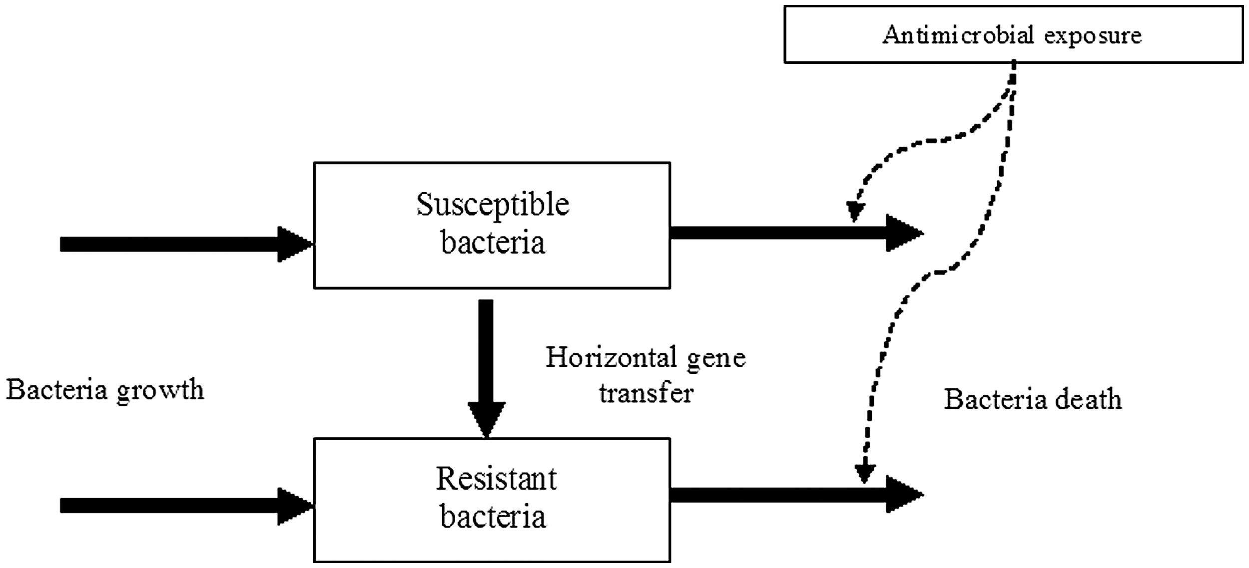
Flow chart for a mathematical model describing antimicrobial resistance dissemination through horizontal gene transfer under antimicrobial exposure. A population dynamic model of the resistant (plasmid-bearing) and susceptible bacteria populations is combined with a pharmacokinetic–pharmacodynamic model that predicts antimicrobial concentration and its effect on bacterial populations. Antimicrobial exposure modifies the bacteria death. Solid arrows indicate flows. Dashed arrows indicate the influence of the antimicrobial exposure on the bacteria death.

FIG. 5.

Simulated change in total bacteria population (solid line) and percentage-resistant bacteria during an antimicrobial treatment (dotted line). The model was parameterized using pharmacokinetic and pharmacodynamic data for the antimicrobial group cephalosporins and Escherichia coli as representative bacteria populations. An intramuscular administration of ceftiofur following label recommendations in cattle was simulated.

Models of antimicrobial resistance dissemination in the host population often assume that infectious individuals are either infected with the sensitive or resistant strain (i.e., they are mutually exclusive). This assumption implies a very strong intraspecific competition among strains. Antimicrobial use and resistance influence competition between sensitive and resistant strains at the host population level. Under treatment, the recovery of hosts that are infected with the sensitive-strain is assumed to be faster. Without antimicrobial exposure, a fitness cost for the resistant strain, which often translates in a faster recovery rate or lower transmissibility, is assumed (Levin, 2001). Abatih et al. (2009) used this approach to evaluate the effect of antimicrobial usage on the transmission of antimicrobial resistant bacteria among pigs. They concluded that control measures that reduce the transmission rate or increase the spontaneous clear-out rate for resistant bacteria would reduce the proportion of pigs with drug-resistant bacteria before transport to slaughter (Abatih et al., 2009). Empirical studies in which transmission of resistant and sensitive strain are measured are needed to validate such conclusions.

Overall, there has been very limited use of mathematical models to understand emergence and dissemination of antimicrobial resistance in food animals. In human medicine, mathematical models have provided useful insights regarding the spread and control of antimicrobial-resistant pathogens in health-care settings (Bonten et al., 2001). A number of independently designed mathematical models have confirmed and quantified the positive effect that general infection control measures such as hand-washing and barrier precautions have in reducing the transmission of antimicrobial resistance bacteria within hospitals (Bergstrom and Feldgarden, 2008). Mathematical models have also demonstrated how some hospital protocols, such as rotating drug classes on a scheduled basis, can actually increase the transmission of antimicrobial-resistant bacteria (Bergstrom et al., 2004).

Conclusions

Mathematical modeling provides a framework to integrate information regarding the transmission and control of foodborne pathogens and antimicrobial resistance. We have shown how mathematical models can be used to (1) understand sources of variation, such as differences in host infectiousness or demographic stochasticity, underlying epidemiological data, (2) evaluate control strategies, and (3) understand mechanisms underlying antimicrobial resistance dissemination.

Linking mathematical models with empirical data provides a robust approach to advance our understanding of foodborne pathogen ecology and evaluate control strategies. Availability of appropriate data to parameterize and validate models has been always one of the most limiting factors in advancing the use of mathematical models. In recent years, advancements in the area of statistical inference and computer science (e.g., Markov chain Monte Carlo methods) have improved the integration between mathematical models and empirical data. These advancements along with a more careful consideration of model data requirements when designing experiments and data collection can readily move forward the application of mathematical models.

Footnotes

Acknowledgments

This project was supported in part by the Cornell University Zoonotic Research Unit of the Food and Waterborne Diseases Integrated Research Network, funded by the National Institute of Allergy and Infectious Diseases, National Institutes of Health, under contract number N01-AI-30054.

Disclosure Statement

No competing financial interests exist.

References

Abatih

, Alban

, Ersbøll

, Lo Fo Wong

. Impact of antimicrobial usage on the transmission dynamics of antimicrobial resistant bacteria among pigs. J Theor Biol, 2009; 256:561–573.

Anderson

, May

. Infectious Diseases of Humans: Dynamics and Control. Oxford: Oxford University Press, 1992.

Andersson

, Hughes

. Antibiotic resistance and its cost: is it possible to reverse resistance? Nat Rev Microbiol, 2010; 8:260–271.

Begon

, Bennett

, Bowers

, French

, Hazel

, Turner

. A clarification of transmission terms in host-microparasite models: numbers, densities and areas. Epidemiol Infect, 2002; 129:147–153.

Bergstrom

, Feldgarden

. The ecology and evolution of antibiotic-resistant bacteria. Evolution in Health and Disease. Stearns

, Koella

. Oxford: Oxford University Press, 2008; 125–137.

Bergstrom

, Lo

, Lipsitch

. Ecological theory suggests that antimicrobial cycling will not reduce antimicrobial resistance in hospitals. Proc Natl Acad Sci U S A, 2004; 101:13285–13290.

Boerlin

, Reid-Smith

. Antimicrobial resistance: its emergence and transmission. Anim Health Res Rev, 2008; 9:115–126.

Bonten

MJM

, Austin

, Lipsitch

. Understanding the spread of antibiotic resistant pathogens in hospitals: mathematical models as tools for control. Clin Infect Dis, 2001; 33:1739–1746.

Callaway

, Anderson

, Edrington

, Elder

, Genovese

, Bischoff

, Poole

, Jung

, Harvey

, Nisbet

. Preslaughter intervention strategies to reduce food-borne pathogens in food animals. J Anim Sci, 2003; 81:E17–E23.

10.

[CDC] Centers for Disease Control and Prevention. Preliminary FoodNet data on the incidence of infection with pathogens transmitted commonly through food-10 states, 2007. Morb Mortal Wkly Rep, 2008; 57:366–370.

11.

Chapagain

, Van Kessel

, Karns

, Wolfgang

, Hovingh

, Nelen

, Schukken

, Grohn

. A mathematical model of the dynamics of Salmonella cerro infection in a US dairy herd. Epidemiol Infect, 2008; 136:263–272.

12.

Collins

. Mycobacterium paratuberculosis: A potential food-borne pathogen? J Dairy Sci, 1997; 80:3445–3448.

13.

Cummings

, Warnick

, Alexander

, Cripps

, Grohn

, McDonough

, Nydam

, Reed

. The incidence of salmonellosis among dairy herds in the Northeastern United States. J Dairy Sci, 2009; 92:3766–3774.

14.

Davis

, Hancock

, Besser

. Multiresistant clones of Salmonella enterica: the importance of dissemination. J Lab Clin Med, 2002; 140:135–141.

15.

Denagamage

, O'Connor

, Sargeant

, Rajić

, McKean

. Efficacy of vaccination to reduce Salmonella prevalence in live and slaughtered swine: a systematic review of literature from 1979 to 2007. Foodborne Pathog Dis, 2007; 4:539–549.

16.

Diekmann

, Heesterbeek

JAP

. Mathematical Epidemiology of Infectious Diseases: Model Building, Analysis and Interpretation. Chichester, UK: John Wiley & Sons, Ltd., 2000.

17.

Fossler

, Wells

, Kaneene

, Ruegg

, Warnick

, Bender

, Eberly

, Godden

, Halbert

. Herd-level factors associated with isolation of Salmonella in a multi-state study of conventional and organic dairy farms: I. Salmonella shedding in cows. Prev Vet Med, 2005a. 70:257–277.

18.

Fossler

, Wells

, Kaneene

, Ruegg

, Warnick

, Bender

, Eberly

, Godden

, Halbert

. Herd-level factors associated with isolation of Salmonella in a multi-state study of conventional and organic dairy farms: II. Salmonella shedding in calves. Prev Vet Med, 2005b. 70:279–291.

19.

Gillespie

. General method for numerically simulating stochastic time evolution of coupled chemical-reactions. J Comput Phys, 1976; 22:403–434.

20.

Gillespie

. Stochastic simulation of chemical kinetics. Annu Rev Phys Chem, 2007; 58:35–55.

21.

Halloran

, Longini

IM.

Jr , Struchiner

. Design and Analysis of Vaccine Studies. New York: Springer, 2009.

22.

Halloran

, Longini

Jr. , Struchiner

. Design and interpretation of vaccine field studies. Epidemiol Rev, 1999; 21:73–88.

23.

Hardman

, Wathes

, Wray

. Transmission of salmonellae among calves penned individually. Vet Rec, 1991; 129:327–329.

24.

Heffernan

, Smith

, Wahl

. Perspectives on the basic reproductive ratio. J R Soc Interface, 2005; 2:281–293.

25.

Heider

, Meiring

, Hoet

, Gebreyes

, Funk

, Wittum

. Evaluation of vaccination with a commercial subunit vaccine on shedding of Salmonella enterica in subclinically infected dairy cows. J Am Vet Med Assoc, 2008; 233:466–469.

26.

House

, Ontiveros

, Blackmer

, Dueger

, Fitchhorn

, McArthur

, Smith

. Evaluation of an autogenous Salmonella bacterin and a modified live Salmonella serotype choleraesuis vaccine on a commercial dairy farm. Am J Vet Res, 2001; 62:1897–1902.

27.

Kabagambe

, Wells

, Garber

, Salman

, Wagner

, Fedorka-Cray

. Risk factors for fecal shedding of Salmonella in 91 US dairy herds in 1996. Prev Vet Med, 2000; 43:177–194.

28.

Keeling

, Rohani

. Modeling Infectious Diseases in Humans and Animals. Princeton, NJ: Princeton University Press, 2008.

29.

Khachatryan

, Besser

, Hancock

, Call

. Use of a nonmedicated dietary supplement correlates with increased prevalence of streptomycin-sulfa-tetracycline-resistant Escherichia coli on a dairy farm. Appl Environ Microbiol, 2006; 72:4583–4588.

30.

Laegreid

, Keen

. Estimation of the basic reproduction ratio (R-0) for Shiga toxin-producing Escherichia coli O157: H7 (STEC O157) in beef calves. Epidemiol Infect, 2004; 132:291–295.

31.

Lanzas

, Brien

, Ivanek

, Lo

, Chapagain

, Ray

, Ayscue

, Warnick

, Grohn

. The effect of heterogeneous infectious period and contagiousness on the dynamics of Salmonella transmission in dairy cows. Epidemiol Infect, 2008a. 136:1496–1510.

32.

Lanzas

, Warnick

, Ivanek

, Ayscue

, Nydam

, Grohn

. The risk and control of Salmonella outbreaks in calf-raising operations: a mathematical modeling approach. Vet Res, 2008b. 39:61.

33.

Lanzas

, Warnick

, James

, Wright

, Wiedmann

, Grohn

. Transmission dynamics of a multi-drug resistant Salmonella typhimurium outbreak in a dairy farm. Foodborne Pathog Dis, 2010; 7:467–474.

34.

Lejeune

, Besser

, Hancock

. Cattle water troughs as reservoirs of Escherichia coli O157. Appl Environ Microbiol, 2001; 67:3053–3057.

35.

Levin

. Minimizing potential resistance: a population dynamics view. Clin Infect Dis, 2001; 33:S161–S169.

36.

Levy

, Marshall

. Antibacterial resistance worldwide: causes, challenges and responses. Nat Med, 2004; 10:S122–S129.

37.

Lili

, Britton

, Feil

. The persistence of parasitic plasmids. Genetics, 2007; 177:399–405.

38.

Lloyd-Smith

, Cross

, Briggs

, Daugherty

, Getz

, Latto

, Sanchez

, Smith

, Swei

. Should we expect population thresholds for wildlife disease? Trends Ecol Evol, 2005a. 20:511–519.

39.

Lloyd-Smith

, Schreiber

, Kopp

, Getz

. Superspreading and the effect of individual variation on disease emergence. Nature, 2005b. 438:355–359.

40.

Lowrance

, Loneragan

, Kunze

, Platt

, Ives

, Scott

, Norby

, Echeverry

, Brashears

. Changes in antimicrobial susceptibility in a population of Escherichia coli isolated from feedlot cattle administered ceftiofur crystalline-free acid. Am J Vet Res, 2007; 68:501–507.

41.

, Grohn

, Smith

, Wolfgang

, Van Kessel

, Schukken

. Assessing the potential impact of Salmonella vaccines in an endemically infected dairy herd. J Theor Biol, 2009; 259:770–784.

42.

, Mitchell

, Smith

, Van Kessel

, Chapagain

, Schukken

, Grohn

. The importance of culling in Johne's disease control. J Theor Biol, 2008; 254:135–146.

43.

, Schukken

, Smith

, Grohn

. Stochastic simulations of a multi-group compartmental model for Johne's disease on US dairy herds with test-based culling intervention. J Theor Biol, 2010; 264:1190–1201.

44.

Lurette

, Belloc

, Touzeau

, Hoch

, Ezanno

, Seegers

, Fourichon

. Modelling Salmonella spread within a farrow-to-finish pig herd. Vet Res, 2008; 39:49.

45.

Martinez

, Baquero

, Andersson

. Predicting antibiotic resistance. Nat Rev Microbiol, 2007; 5:958–965.

46.

Naidan

, Sonia

, Orhan

, Jun

, Shouxiong

, Linda

, Qijing

. Enhanced in vivo fitness of fluoroquinolone-resistant Campylobacter jejuni in the absence of antibiotic selection pressure. Proc Natl Acad Sci U S A, 2005; 102:541–546.

47.

[NRC] National Research Council. Diagnosis and Control of Johne's Disease. Washington, DC: The National Academies Press, 2003.

48.

Ogden

, MacRae

, Strachan

. Is the prevalence and shedding concentrations of E. coli O157 in beef cattle in Scotland seasonal? FEMS Microbiol Lett, 2004; 233:297–300.

49.

Oliver

, Wiedmann

, Boor

. Environmental reservoir and transmission into the mammalian host. In: Listeria monocytogenes. Pathogenesis and Host Response. Goldfine

, Shen

. New York: Springer, 2007; 111–137.

50.

Oliver

, Patel

, Callaway

, Torrence

. ASAS Centennial Paper: developments and future outlook for preharvest food safety. J Anim Sci, 2009; 87:419–437.

51.

Otto

, Day

. A Biologist's Guide to Mathematical Modeling in Ecology and Evolution. Princeton, NJ: Princeton University Press, 2007.

52.

Robinson

, Brown

, Wright

, Hart

, French

. Quantifying within- and between-animal variation and uncertainty associated with counts of Escherichia coli O157 occurring in naturally infected cattle faeces. J R Soc Interface, 2009; 6:169–177.

53.

Salyers

, Gupta

, Wang

. Human intestinal bacteria as reservoirs for antibiotic resistance genes. Trends Microbiol, 2004; 12:412–416.

54.

Smith

, Moxley

, Peterson

, Klopfenstein

, Erickson

, Bretschneider

, Berberov

, Clowser

. A two-dose regimen of a vaccine against type III secreted proteins reduced Escherichia coli O157:H7 colonization of the terminal rectum in beef cattle in commercial feedlots. Foodborne Pathog Dis, 2009; 6:155–161.

55.

Stanford

, Croy

, Bach

, Wallins

, Zahiroddini

, McAllister

. Ecology of Escherichia coli O157:H7 in commercial dairies in Southern Alberta. J Dairy Sci, 2005; 88:4441–4451.

56.

Thomas

, Klinkenberg

, Ejeta

, Van Knapen

, Bergwerff

, Stegeman

, Bouma

. Quantification of horizontal transmission of Salmonella enterica Serovar Enteritidis bacteria in pair-housed groups of laying hens. Appl Environ Microbiol, 2009; 75:6361–6366.

57.

Torrence

. Epidemiology and food safety. Foodborne Pathog Dis, 2005; 2:2–11.

58.

Turner

, Begon

, Bowers

, French

. A model appropriate to the transmission of a human food-borne pathogen in a multigroup managed herd. Prev Vet Med, 2003; 57:175–198.

59.

van den Driessche

, Watmough

. Reproduction numbers and sub-threshold endemic equilibria for compartmental models of disease transmission. Math Biosci, 2002; 180:29–48.

60.

Van Schaik

, Klinkenberg

, Veling

, Stegeman

. Transmission of Salmonella in dairy herds quantified in the endemic situation. Vet Res, 2007; 38:861–869.

61.

Varma

, Molbak

, Barrett

, Beebe

, Jones

, Rabatsky-Ehr

, Smith

, Vugia

, Chang

HGH

, Angulo

. Antimicrobial-resistant nontyphoidal Salmonella is associated with excess bloodstream infections and hospitalizations. J Infect Dis, 2005; 191:554–561.

62.

Weigel

, Nucera

, Qiao

, Teferedegne

, Suh

, Barber

, Bahnson

, Isaacson

, White

. Testing an ecological model for transmission of Salmonella enterica in swine production ecosystems using genotyping data. Prev Vet Med, 2007; 81:274–289.

63.

Woolhouse

MEJ

, Dye

, Etard

, Smith

, Charlwood

, Garnett

, Hagan

, Hii

JLK

, Ndhlovu

, Quinnell

, Watts

, Chandiwana

, Anderson

. Heterogeneities in the transmission of infectious agents: implications for the design of control programs. Proc Natl Acad Sci U S A, 1997; 94:338–342.

64.

Yan

, Gilbert

. Antimicrobial drug delivery in food animals and microbial food safety concerns: an overview of in vitro and in vivo factors potentially affecting the animal gut microflora. Adv Drug Delivery Rev, 2004; 56:1497–1521.

65.

Zhang-Barber

, Turner

, Barrow

. Vaccination for control of Salmonella in poultry. Vaccine, 1999; 17:2538–2545.

66.

Zhang

, Sahin

, McDermott

, Payot

. Fitness of antimicrobial-resistant Campylobacter and Salmonella. Microb Infect, 2006; 8:1972–1978.

Supplementary Material

Please find the following supplemental material available below.

For Open Access articles published under a Creative Commons License, all supplemental material carries the same license as the article it is associated with.

For non-Open Access articles published, all supplemental material carries a non-exclusive license, and permission requests for re-use of supplemental material or any part of supplemental material shall be sent directly to the copyright owner as specified in the copyright notice associated with the article.

0.00 MB

0.35 MB