
Abstract
Abstract
Youk, Ada O., Jeanine M. Buchanich, Jon Fryzek, Michael Cunningham, Gary M. Marsh. An ecological study of cancer mortality rates in high altitude counties of the United States. High Alt. Med. Biol. 13:98–104.—To test the hypothesis that sustained, increased hemoglobin levels as measured by residence in high altitudes lead to an increase of malignant cancer deaths, we performed an assessment of U.S. cancer mortality rates for people residing in high altitude counties compared with those in counties with altitudes close to sea level. This included a graphical analysis of mortality rates for all cancers, female breast cancer, respiratory system cancer (RSC) and non-Hodgkin lymphoma (NHL), computation of standardized mortality ratios (SMRs) and Poisson regression modeling. Overall, our ecological evaluation showed statistically significantly reduced SMRs and rate ratios (RRs) for high altitude residents compared to sea level residents. For the causes of death categories examined, we found no evidence that persons residing in high altitude counties are at an elevated risk of cancer mortality compared with persons living close to sea level. Our results corroborate previous altitude studies of cancer mortality.
Introduction
Elevation is defined as the height of the natural land above sea level although there is no standard definition for what elevations are considered “high” altitude. Most sources consider high altitude as any elevation greater than 1524 m (Zafren & Honigman, 1997; Heinicke et al., 2005; Leon-Velardi et al., 2005). Minor physiological effects are seen at around 1524 m, start to worsen around 2134 m and large effects (severe altitude sickness) are seen at greater than 3505 m. One of the physiological effects of living in a high altitude area is an increased level of hemoglobin (Zafren & Honigman, 1997; Leon-Velardi et al., 2005). To test the hypothesis that increased, sustained hemoglobin levels as measured by residence at high altitudes lead to death from cancer, we performed an assessment of cancer mortality rates for individuals residing in high altitude counties compared to those who reside in counties with altitudes close to sea level. We show here the results of this ecological evaluation of United States (U.S.) cancer mortality for all cancers, breast cancer, respiratory system cancer and non-Hodgkin lymphoma (NHL). These cancers were chosen as they have been associated with adverse events in several recent clinical trials of ESAs (Khuri, 2007; Bennet et al., 2008).
Methods
Determine the U.S. counties at high altitudes
We defined high altitude as elevations greater than 2134 m, the point at which physiological effects start to worsen. We first screened the contiguous United States for states with high point (peak) elevations greater than 2134 m (US Geological Survey, 1983). There are 13 states in the contiguous United States with a high point elevation above 7000 feet (Arizona, California, Colorado, Idaho, Montana, Nevada, New Mexico, Oregon, South Dakota, Texas, Utah, Washington and Wyoming). From these 13 states, we determined which counties were considered to be high altitude.
While mean elevations by U.S. county are available by merging latitude and longitude coordinates of the center of each U.S. county with the National Elevation Database, they do not take population size into consideration. Because of our focus on cancer mortality rates, we used the mean elevation of the most populous city in every county in each of the 13 states to estimate the altitude of the county (Amsel et al., 1982). Utilizing the most populous city (versus the overall mean county elevation) based our estimate of altitude on where people lived. There were 31 counties that met the high altitude criteria of elevation greater than 2134 m. Estimates of elevations were abstracted from the U.S. Census (American Fact Finder, 2008) and the U.S. Geological Survey (1983).
Selection of comparison counties
Per the U.S. Census Bureau, there are 3,144 counties in the United States. Comparison counties were defined as those counties with estimated mean elevation less than 1000 ft. Because areas close to sea level are more densely populated than those at high altitudes, we used 305 m as the cutoff for low altitude to allow for more potential matches in the possible comparison counties. Using altitudes less than 305 m, provided us with a comparison group which was free of altitude related physiological changes as these usually start to occur at altitudes greater than 1524 m (Leon-Velarde et al., 2005). Comparison county elevations were estimated using the same process as the high altitude counties. To attempt some control for possible confounding, we selected comparison counties based on county to county frequency matching controlling for geographical area and socioeconomic status (SES). For the geographical area criteria, we attempted to get a same state or adjacent state match; however that was not always possible. Comparison counties were at most two states away from their high altitude county match. We used median household income and percent population below the poverty level (both based on the 2000 U.S. census via American Fact Finder) as surrogates for SES. We chose the first county that met the criteria of the matching for the comparison county. A similar selection process was performed successfully in an ecologic study of cancer in Kanawha county West Virginia (Day et al., 1992; Talbott et al., 1992).
Generation of cancer mortality rates
We used the Mortality and Population Data System (MPDS) (Marsh et al., 2007) to generate the cancer mortality rates for the a priori causes of interest (mortality from all cancers (International Classification of Disease (ICD) 9th revision codes 140-209), respiratory system cancer (ICD 9th revision codes 160-165), female breast cancer (ICDA 9th revision code 174), and non-Hodgkin lymphoma (ICD 9th revision codes 200, 202.0-202.1, 202.8-202.9). Since 1980, the Department of Biostatistics at the University of Pittsburgh has maintained a data repository and retrieval system for detailed mortality data provided by the National Center for Health Statistics and the U.S. Census Bureau. This Mortality and Population Data System (MPDS) contains the underlying cause of death code (using International Classification of Diseases (ICD) four-digit codes in effect at the date of death) for all persons who died in the United States between 1950 and 2004. Individual death records include codes for sex, race, age of death, year of death and geographic location (county and state of residence at time of death). The MPDS contains over 110 million deaths in the United States. In MPDS, individual death records are categorized and linked with the corresponding population data to form death rates specific for five-year age groups, five-year time periods, race (white and non-white), sex, geographic location, and cause of death.
For the graphical analyses, age-adjusted rates were generated for each cause of interest along with associated estimates of standard error. Rates were generated for the aggregates of counties within each altitude group (high altitude vs low altitude). The age-adjusted rates were computed using the U.S. 2000 total population as the weighting population. For the statistical analyses, we generated unadjusted age-time-sex-race specific rates for each cause of interest. The time period covered by the rates was 1950–2004.
Data analysis
The analysis was comprised of descriptive and statistical analyses of the cancer mortality rates in high altitude counties compared to low altitude counties with control for potential confounding factors such as age, time, race, sex, SES, and geographic area.
We performed a graphical analysis of the age-adjusted cancer mortality rates in the high altitude counties as compared to the low altitude counties for each of the 5-year time periods. Graphs were created over all race/sex groups for each cause of interest and included 95% confidence intervals for the age-adjusted rates for each time period. These comparisons do not account for the matching of low altitude county to high altitude county.
To facilitate comparisons of the mortality rates (expressed as mortality excesses and deficits) and to utilize the matching, we computed Standardized Mortality Ratios (SMRs). The expected number of deaths used in the SMR was computed as the product of the age-time-race-sex specific cancer mortality rates of the low altitude county and the population of the high altitude county. SMRs for total cancer and cause-specific cancer mortality were computed overall and for subcategories based on race/gender, age group, time period, and categories of high altitude (2134–2438 m, 2439–2742 m, 2743 m+). We used the exact Poisson distribution to assess the statistical significance of SMRs that deviated from their null (baseline) value of 1.0 (where the observed and expected numbers of cases or deaths are equal).
Multi-variate analyses of the cancer mortality rates were also performed. We used Poisson regression (Breslow & Day, 1987; Frome & Checkoway, 1985) to estimate adjusted risk (rate) ratios. Altitude level was the predictor of interest and was treated several ways. We dichotomized altitude as high and low and also formed ordinal categories of the high altitude group.
In Poisson regression, the observed number of deaths in a particular cross-classification of the variables is assumed to follow a Poisson distribution with a mean that depends on the persons at risk and the effects of the classification factors. A multiplicative model for the mortality rates is given by: log E (observed deaths)=log (persons)+β’x, where E denotes statistical expectation, log denotes natural logarithm, β is a p-dimensional vector of regression coefficients to be estimated and x is the corresponding vector of covariates. The persons at risk are treated as an offset (known quantity) in the models.
We fit multivariate models for altitude adjusting for the effects of the potential confounders (sex, race, age group, and time period) for each cause of interest. We obtained maximum likelihood estimates of Poisson regression parameters using STATA (STATA, 2007). We adjusted SMRs for multiple comparisons using Bonferroni-adjusted significance levels (Miller, 1991).
Results
Graphical analysis
Figures 1–4 show the age-adjusted rates by five year time periods for the high altitude counties and the comparison counties for each cause of death of interest. In Fig. 1, the rates of all cancer mortality are consistently lower for the high altitude counties than the comparison counties across the full time period. These differences are statistically significant as the confidence intervals do not overlap. The graph for female breast cancer (Fig. 2) also shows that the rates are consistently lower for the high altitude counties. However, only the rate differences between high altitude and low altitude counties are statistically significant in the 1955–1959, 1965–1969 and 1970–1974 time periods. The confidence intervals are wider than all cancer mortality due to the smaller numbers of observed deaths in each time period. Figure 3 shows the NHL rates consistently increase over time for both the high altitude and low altitude groups. The differences between the two county groups are lower for high altitude across the entire time period. These are statistically significant for time periods 1975–1979, 1980–1984 and 1995–1999 time periods. Figure 4 shows the RSC rates are consistently lower for the high altitude counties when compared to the low altitude counties for the time period 1950–2004. As with all cancer, these differences are statistically significant as shown by the non overlapping confidence intervals. The rates in the low altitude group consistently increase up to 1995, when they start to eventually decline. However, in the high altitude group, the rates increase to 1980 and then are consistently level.
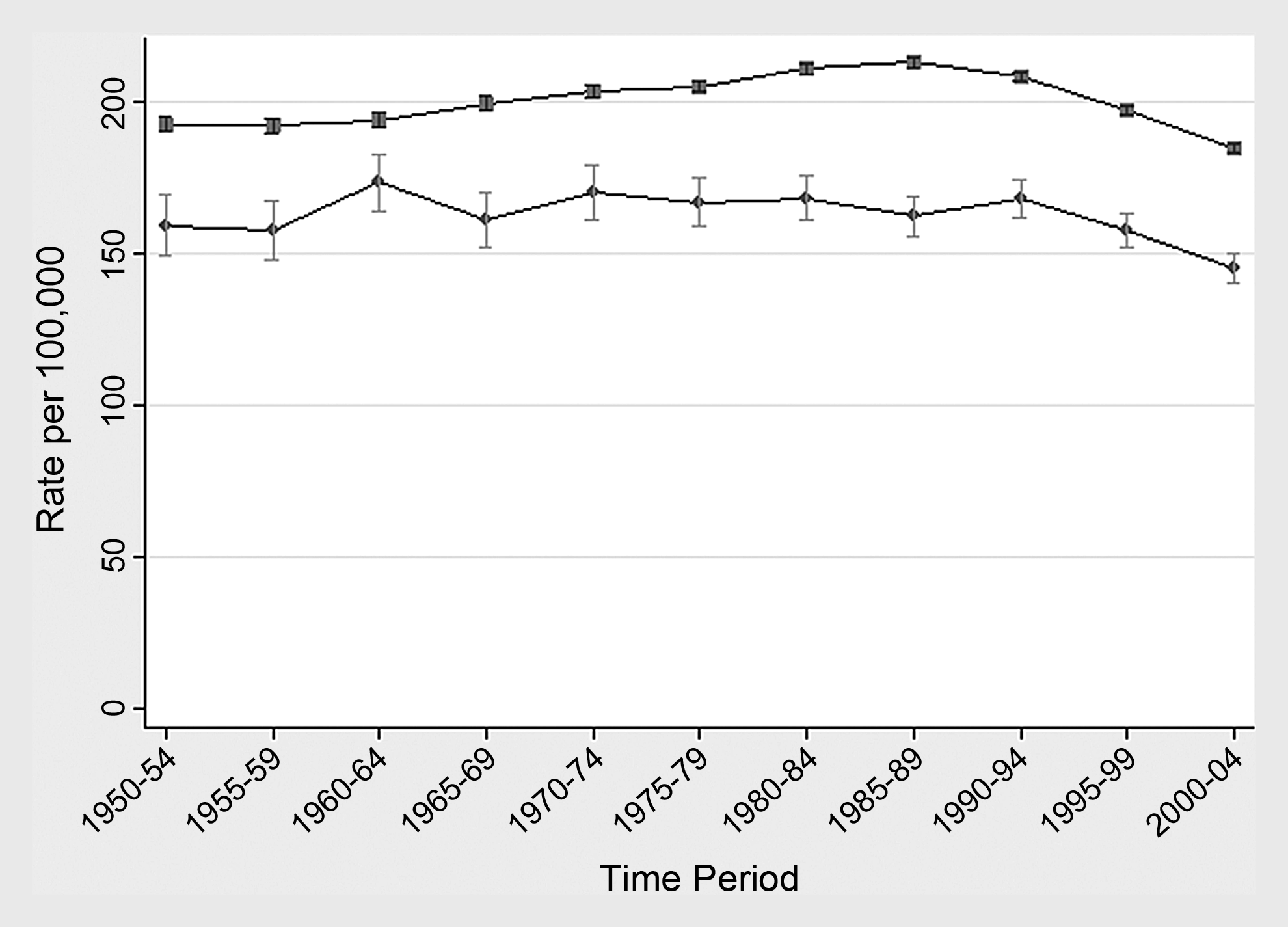
Comparison of age-adjusted all cancer mortality rates with 95% confidence intervals for U.S. counties at elevations greater than 2134 m to matched control counties at elevations less than 305 m. Control counties were matched on geographic area and two surrogates of socioeconomic status (median household income and % below the poverty level; both based on the 2000 U. S. Census). County elevation: • 2134 m+, ▪<305 m.
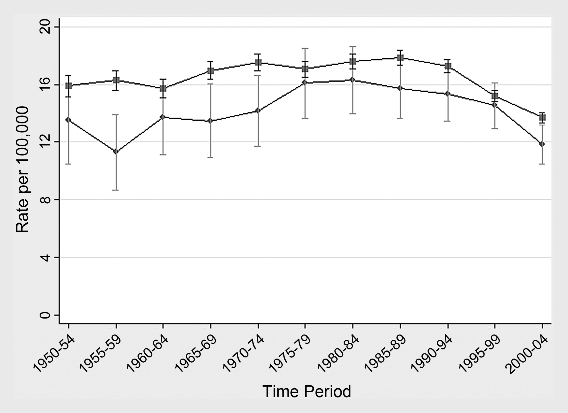
Comparison of age-adjusted breast cancer mortality rates with 95% confidence intervals for U.S. counties at elevations greater than 2134 m to matched control counties at elevations less than 305 m. Control counties were matched on geographic area and two surrogates of socioeconomic status (median household income and % below the poverty level; both based on the 2000 U. S. Census). County elevation: • 2134 m+, ▪<305 m.
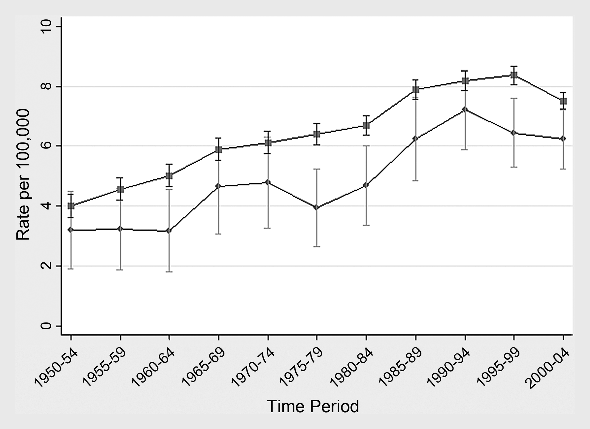
Comparison of age-adjusted non-Hodgkin's lymphoma mortality rates with 95% confidence intervals for U.S. counties at elevations greater than 2134 m to matched control counties at elevations less than 305 m. Control counties were matched on geographic area and two surrogates of socioeconomic status (median household income and % below the poverty level; both based on the 2000 U. S. Census). County elevation: • 2134 m+, ▪<305 m.
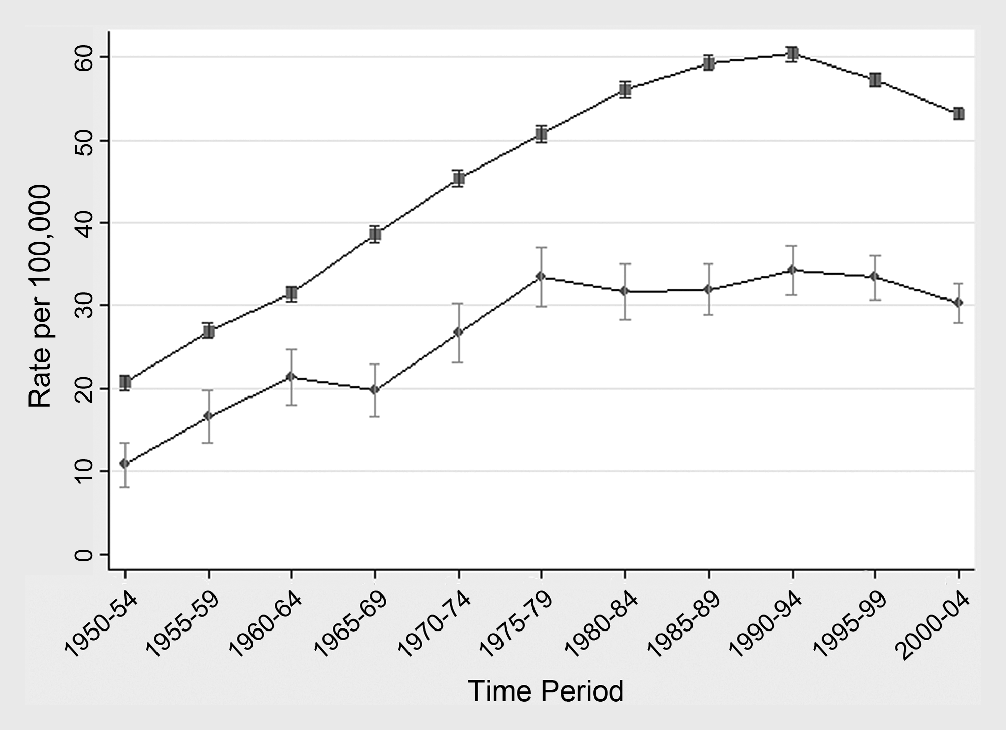
Comparison of age-adjusted respiratory system cancer mortality rates with 95% confidence intervals for U.S. counties at elevations greater than 2134 m to matched control counties at elevations less than 305 m. Control counties were matched on geographic area and two surrogates of socioeconomic status (median household income and % below the poverty level; both based on the 2000 U. S. Census). County elevation: • 2134 m+, ▪<305 m.
Standardized mortality ratios
Tables 1–4 show the SMRs by study factor. For all cancer (Table 1), the high altitude counties have consistently lower all cancer mortality when compared with the low altitude counties and there appears to be no patterns across the levels of high altitude. There was a slight increasing trend in SMRs across levels of age at risk for altitude group 2439–2742 m, however all of the SMRs were statistically significantly reduced. There were several small elevations by time period in the 2439–2742 m group (1950–1959 SMR=1.15, 95% CI=.96–1.37; 1960–1969 SMR=1.04, 95% CI=.87–1.24) and 2743 m+ (1960–1969 SMR=1.05, 95% CI=.87–1.26; 1970–1979 SMR=1.01, 95% CI=.86–1.19), although none were statistically significant. For all altitude levels, the SMRs tended to decline over time.
p<.05.
p<.01.
For female breast cancer (Table 2), results are mostly similar to the all cancer mortality. There were slight increasing trends in SMRs across levels of age at risk for all of the altitude groups and overall, however all but two of the SMRs were deficits indicating less risk of breast cancer mortality for the high altitude group. Of the elevations seen, none were statistically significant and no consistent patterns emerged across altitude levels.
p<.05.
p<.01.
For NHL (Table 3), there was an overall statistically significant 22% deficit in mortality when comparing high altitude counties to those at sea level (SMR=0.78, 95% CI=.72–.85). All of the NHL SMRs by study factor were reduced when collapsed across altitude level. The SMRs by study factor for the 2134–2435 m altitude group were all deficits and most were statistically significant. Several moderate to large excesses for certain time periods were also seen in the higher altitude groups but none were statistically significant. For those aged <45 and 65+ in the highest altitude group, SMRs were elevated but not statistically significant (<45 SMR=1.36, 95% CI=0.65–2.50; 65+ SMR=1.12, 95% CI=.72–1.65).
p<.05.
p<.01.
For RSC (Table 4), the high altitude counties had consistently lower mortality when compared with the low altitude counties. There appears to be no patterns across the levels of high altitude except for the first time period (1950–1954) group. Here, SMRs increase with increasing levels of altitude (2134–2435 m SMR=0.62, 2439–2742 m SMR=0.94, 2743 m+ SMR=1.13), although none were statistically significant. There was a slight increasing trend in SMRs across levels of age at risk for altitude group 2439–2742 m, however all of the SMRs were statistically significantly reduced. There were several small elevations by time period in the 2439 m+ groups, although none were statistically significant. For the most part, the SMRs tended to decline over time for all altitude levels and overall. We found that the statistical significance of the SMRs overall in Tables 1–4 was relatively invariant to Bonferroni-adjusted p-values, leading us to the same overall conclusions regarding mortality in relation to altitude.
p<.05.
p<.01.
Poisson regression
Table 5 shows the results of the Poisson regression modeling for the causes of interest. All of the adjusted rate ratios (RRs) were reduced for every cause of death, suggesting lower mortality in the high altitude counties than the comparison counties. Except for the 2439–2742 m altitude level for NHL, all RRs were statistically significant. The model for NHL showed a slightly increasing trend of risk across increasing levels of altitude, although all of the RRs were reduced.
All models were adjusted for sex, race, age group (<45, 45–64, 65+), and time period (1950–1959, 1960–1969, 1970–1979, 1980–1989, 1990–1999, 2000–2004).
Models for breast cancer were not adjusted for sex as they were based only on females.
Discussion
Our analysis of the association between altitude of residence and cancer mortality from total, female breast, NHL or RSC cancers found no evidence that people in high altitude counties are at increased risk for mortality from these diseases. In fact, for the most part, our comparisons found statistically significantly reduced SMRs and RRs for residents in high altitude counties compared to sea level counties. There were several isolated elevations in the SMR analysis that existed for breast cancer mortality risk. These elevated SMRs were seen in ages 65+ and from 1950–1989 in the 2134–2438 m group as well as in several time periods in the higher elevation groups, although there did not appear to be any consistent patterns.
These analyses expanded upon previous evaluations and our findings are similar to those in other published studies (Amsel et al., 1982; Mason et al., 1974; Weinburg et al., 1987). Mason et al. (1974) compared cancer mortality in 53 U.S. counties with a majority of the altitudes greater than 914 m to the total U.S. and rural counties in the United States to assess whether there was an association between levels of background radiation (which increases with increasing altitudes) and cancer. They found no consistent evidence of an increased risk of leukemia mortality or mortality from all cancers (minus leukemia) for the time period 1950–1969. In fact, the largest elevations noted were for comparisons of two counties at sea level to the total United States. Similar results were seen when the comparisons were made to rural U.S. counties. The authors attributed the lower mortality rates at the high altitudes to “rurality” rather than being a function of altitude however, there was no attempt to control for confounding. Another study (Amsel et al., 1982), found lower mortality rates at high altitudes for cancers of the tongue and mouth, esophagus, larynx, lung and all cancers for the time period 1950-69. The findings were consistent across gender, levels of industrialization, urbanization and ethnicity. They hypothesize that levels of cellular pH, which controls protein synthesis and mitosis in tumor cells, at high altitudes may make cancer cells less likely to grow. Weinburg et al. (1987) also found that mortality was negatively related to altitude for cancers of the trachea, bronchus, and lung, stomach, small or large intestine, female breast, multiple myeloma, and leukemia during the time period 1960–1969. They suggest that because oxygen may produce toxic effects at physiologic levels, the altitude effect seen may reflect interaction between oxygen levels and background radiation. A more recent study found lower all cause mortality in U.S. dialysis patients who resided at high altitudes compared to those who lived in low altitude areas. They found a monotonic increase in survival rates across altitude levels with or without control for potential confounding variables and co-morbid conditions suggesting that increased altitude is associated with reduced mortality (Winkelmayer et al., 2009).
One of the main ways in which people acclimate to high altitude is through increased hemoglobin levels to allow more efficient transport of oxygen (Hurtado, 1960). This action is similar to the effect of ESAs given for the treatment of chemotherapy-induced anemia. While some clinical trial reviews have suggested an increased risk of death, particularly due to lung cancer, in patients treated with ESAs (Khuri, 2007;Bennet et al., 2008), our ecologic analysis of persons residing in high altitude counties, with high hemoglobin levels, found no evidence of increased cancer risk compared to people living at low altitude counties.
Our analysis has several limitations inherent to the study of grouped data due to the ecologic nature of the evaluations. We are comparing populations, rather than looking at individuals, so are making assumptions about the characteristics of the deaths. It is difficult to control for confounding in these types of analyses. However, we matched the counties on SES and geographic area to help obviate differences in some factors related to the development of cancer. We are assuming that there are no environmental factors (such as background radiation) other than altitude that are affecting the SMRs and RRs. Another limitation is the use of high altitude as a proxy for increased hemoglobin levels which assumes that the residents of high altitude counties have higher hemoglobin levels than residents of low altitude counties.
Our analysis has several strengths. This evaluation was a quick and reasonable way to address the question of increased cancer mortality in high altitude counties. It would have been much more difficult and costly, perhaps even infeasible, to obtain hemoglobin levels on individuals residing in high and low altitude counties and follow them until a cancer death occurred. This study extended similar older studies to examine more current mortality data through 2004; the previous studies only evaluated the more limited 1950–1969 time period. We also obviated some of the problems with ecologic studies by attempting to control for confounding, examining only a limited number of cancers with a potential association between hemoglobin and tumor progression (Morgenstern, 1982), matching counties on the basis of SES and geographic area, and utilizing multivariate Poisson regression modeling. These techniques are standard analyses in the investigation of ecologic data. Additionally, the computation of the mortality rates was very straightforward using the MPDS system.
Conclusion
Our analysis of the association between altitude of residence and cancer mortality from total, female breast, NHL, or RSC cancers found no evidence that persons residing in high altitude counties are at an elevated risk of mortality from these diseases compared with persons living close to sea level. These results corroborate previous altitude studies of cancer mortality.
Footnotes
Disclosures
Jon Fryzek was employed by Amgen, Inc. at the time of this study. Ada Youk, Jeanine Buchanich, Michael Cunningham, and Gary Marsh disclosed no conflicts of interest or financial ties.
Amgen, Inc. sponsored this research, but the design, conduct, analysis, and conclusions are those of the authors.