Efficient Aircraft Rerouting During Commercial Space Launches

Abstract

Currently, during a commercial space launch, the Federal Aviation Administration prohibits air traffic within a large column of airspace around the launch trajectory. The prohibited airspace is often active for hours at a time, resulting in hundreds of rerouted flights. Recent research has focused on making the prohibited airspace dynamic throughout the commercial space launch and limiting the geographical extent. This article uses a Markov decision process to model the problem and dynamic programming to solve for an optimal rerouting policy. The resultant policy produces smaller prohibited regions and could provide real-time reroutes for air traffic controllers to relay to pilots during a commercial space launch. This article presents example policies that more efficiently reroute aircraft during commercial space launches without compromising safety.

Introduction

On February 6, 2018, the SpaceX Falcon Heavy was launched out of Kennedy Space Center, disrupting 563 flights with an average delay of 8 min and flight course deviation of 62 NM.¹ It is predicted that on average, each disrupted flight incurred an additional expense of $547.84 due to fuel, labor, and aircraft expenses. Not including missed connections, a single commercial space launch costs commercial airlines more than $308,000.² The delay and reroute source from that the Federal Aviation Administration (FAA) prohibits air traffic within a large, indefinite altitude, column of airspace around the launch trajectory. Depending on the launch schedule, this prohibited region can be active for hours causing many flights to be rerouted.

Historically, these conservative airspace restrictions have caused limited disruption because launches were infrequent. From 2013 to 2017, there was a 350% increase in commercial space launches, and it is predicted that these will continue to increase.¹ Furthermore, the introduction of suborbital reusable vehicles will potentially increase the commercial space launch rate by a factor of 50 and introduce additional launch facilities in dense air traffic regions.³ The increases in launch frequency make the current airspace restrictions expensive and infeasible in the future.

To address the increase in airspace disruptions and minimize added airline costs, we suggest moving from the static prohibited regions⁴ toward a dynamic process. Methods such as compact envelopes⁵ and space transition corridors^6,7 use probabilistic risk analysis to create dynamic restricted regions, but neither of these methods explicitly directs air traffic controllers how to reroute the aircraft. We present a technique to reroute aircraft directly that involves modeling the problem as a Markov decision process (MDP).⁸

In an MDP, an agent chooses an action at each time step based on the observed state. During a commercial space launch, the action is a reroute command that ensures aircraft safety and promotes airspace efficiency by considering the following: a model of commercial space launch trajectory, the probability of anomaly during the modeled launch, the corresponding debris trajectory if an anomaly occurs, the potential aircraft locations, the potential aircraft headings, and the aircraft maneuvering capabilities. The remainder of this article describes how using an MDP framework to produce optimal rerouting commands can lead to greater efficiency during a commercial space launch.^9,10

Commercial Space Launch Scenario

To present this concept, we model a hypothetical two-stage to orbit commercial space launch out of Kennedy Space Center interacting with air traffic at 35,000 ft. A snapshot of the air traffic in this region is shown in Figure 1.¹¹ To model the problem, we consider the probability of anomaly and its resultant debris field. We calculate the expected debris field for each potential time of anomaly that will produce debris in the airspace within 10 min. We model the debris from the publicly available and comprehensive Columbia disaster debris catalog,¹² which separates the debris into 11 categories based on weight, ballistic coefficient, and size and includes the expected number of pieces of debris for each category. Many of the pieces of debris have similar trajectories, so we model only a representative set of ∼4,000 pieces of debris.⁵

Fig. 1.

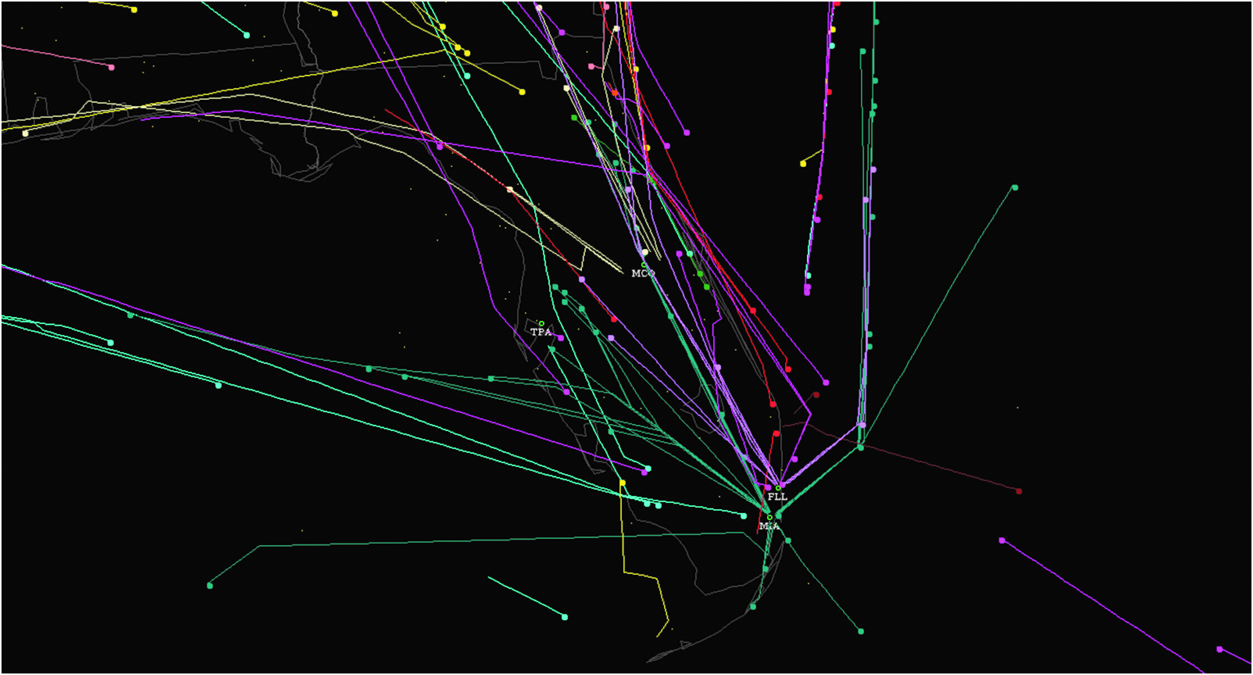
A snapshot of flights around Kennedy Space Center.

The debris is modeled using Range Safety Assessment Tool (RSAT)¹³ with atmosphere profiles provided by the MIT Lincoln Laboratory. The atmosphere profile includes mean air density, air density standard deviation, wind velocities, and wind velocity standard deviations from 1 to 25 km. Figure 2 shows example debris trajectories.

Fig. 2.

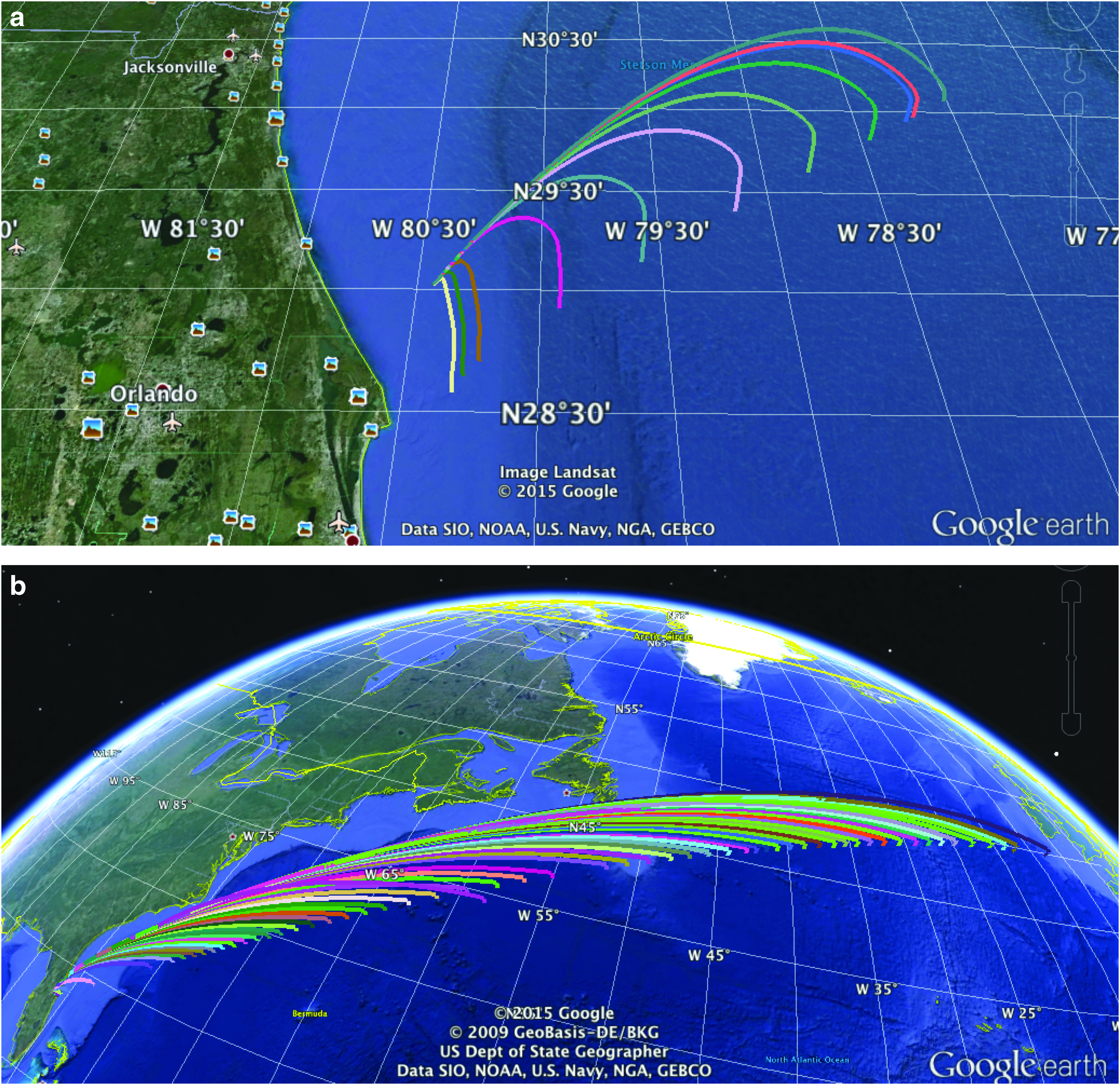
Example debris trajectories. (a) One piece of debris from the 11 types after an anomaly at 100 s. (b) One piece of debris from one type of debris after an anomaly at varying time steps.

Modeling

An MDP is used to formulate sequential decision problems by breaking the problem into four components: state space, action space, transition function, and reward function.^8,14 An example of a small MDP is shown in Figure 3. This example has three states (1, 2, and 3) and two potential actions available at each state (A and B). For each state/action pair, the next state is determined probabilistically as denoted by the probability on the line connecting the action to next state, such as 90% of the time taking action A from state 1 results in transitioning to state 2 and 10% of the time you stay in state 1. The values associated with the orange arrows denote the rewards (or costs) for transitioning between two states with a specific action such as the +1 reward from taking action A in state 2 and transitioning to state 1.

Fig. 3.

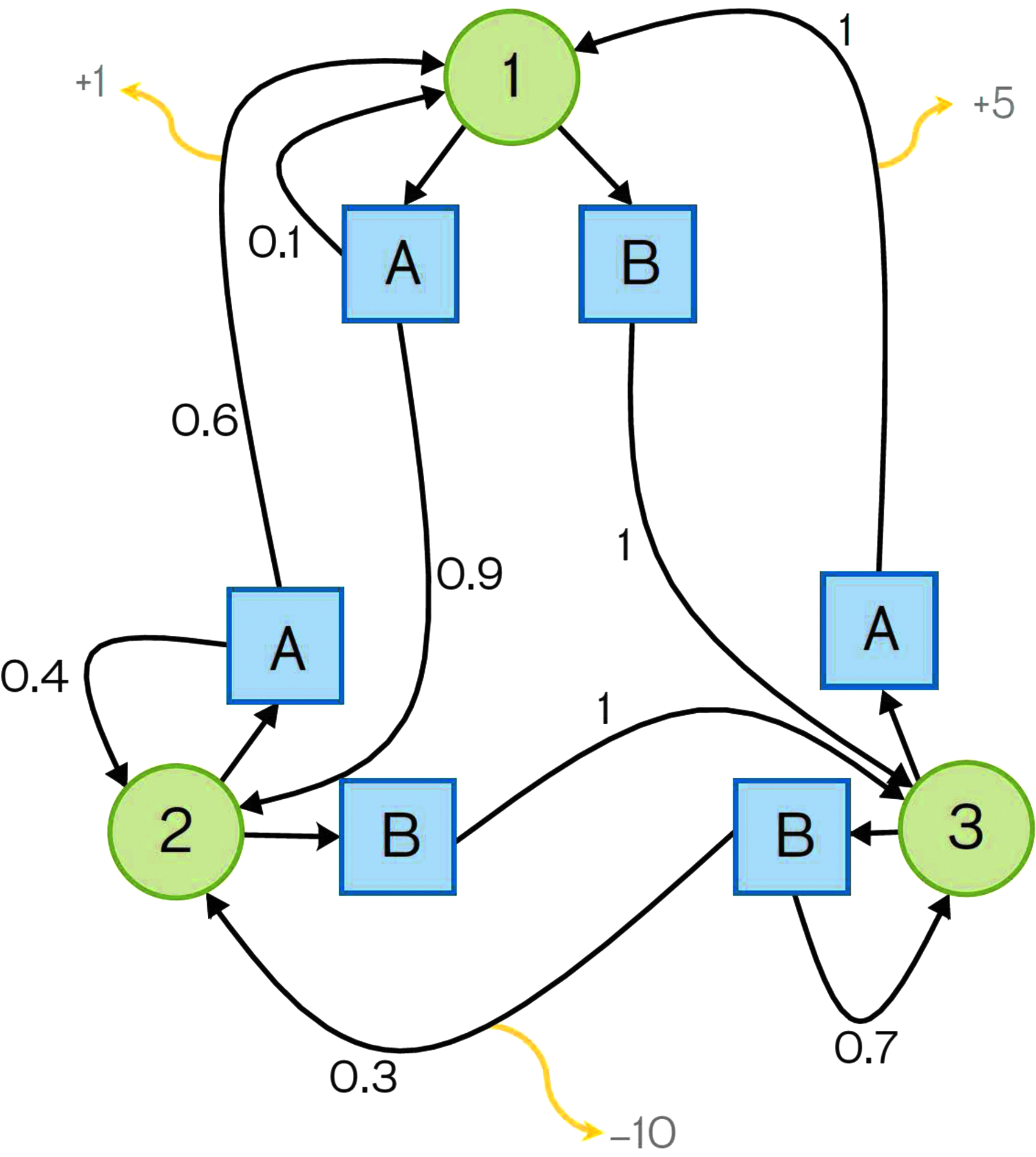
An example MDP formulation. MDP, Markov decision process.

An optimal solution to an MDP is a policy that maximizes the accumulation of the expected rewards (or minimizes the accumulation of expected costs) when followed. The same principles presented in this small problem can be applied to the problem of rerouting aircraft during a commercial space launch.

State Space

The state space is denoted S. A state s ∈ S captures the aircraft position (east, e, and north, n), aircraft heading (ψ), time of anomaly (t_anom), and time since launch (t). The two time variables are used to gather information about debris locations. All of the state space variables are discretized using a five-dimensional grid.

Action Space

The action space is denoted A. An action a ∈ A is a reroute command provided to the pilots. The action space contains strong left (−30°), weak left (−15°), maintain (0°), no advisory (nil), weak right (15°), and strong right (30°). The turn commands represent standard rate and half standard rate turns.

Transition Function

The transition model is denoted T, where T(s′ | s, a) is the probability of transitioning to state s′ after taking action a from state s. The transition function captures uncertainty in pilot response, aircraft trajectory, launch vehicle health, and potential debris.

The e, n, and ψ components of the state are updated based on the reroute command. Since we do not model a specific flight path, when an aircraft is commanded _NIL, the pilot is modeled to follow a discretized normal distribution. If the aircraft is commanded to maintain heading, the pilot is modeled to always maintain the current heading. If the aircraft is commanded a different action, the pilot has an average response time of 20 s. The updated heading and aircraft heading are used to deterministically update the e and n position. The t_anom component of the state is updated once such that an anomaly occurs 50% of the time during the first stage of launch. The t component of the state is updated deterministically in 10 s increments.

Reward Function

The immediate reward of an aircraft in state s taking action a and ending up in new state s′ is denoted R(s, a, s′). The reward function for rerouting aircraft is set up as safety and efficiency costs. The safety cost of 1 is incurred when the aircraft is within a threshold from a piece of debris or the launch vehicle. For this investigation, the threshold is set to match the definition of a near midair collision between two aircrafts.¹⁵ The efficiency cost is incurred when the aircraft is commanded any action besides _NIL and proportional to the strength of the action of at most 1. The safety and efficiency costs are added together with an experimentally found scaling factor.

Solution Techniques

Given the MDP model, we can solve for a policy that tells us the best action to execute from every possible state that minimizes expected total cost. We walk through a simplified example focusing on a subset of the state space with a single piece of debris that falls through the airspace at t = 100 s. Figure 4a shows 35 cells representing 35 states that exist in a subset of the possible aircraft east and north states. The star represents the state where the debris passes through the airspace. At t = 100 s, only the cell containing the debris has a large cost due to the safety threshold violation, as represented by the red in Figure 4a. Now, we can solve for the values of the states one time step earlier, t = 90 s.

Fig. 4.

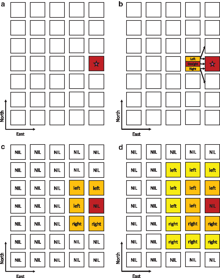
Example of solving for an optimal policy for a single piece of debris. (a) Subset of state space at t = 100 s. (b) Subset of state space at t = 90 s showing the transition function. (c) Example policy at t = 90 s. (d) Example policy at t = 80 s.

For the example, we first do this for an aircraft located in the grid cell immediately to the left of the debris, flying toward the debris (ψ = 0°), with the limited commands: right, left, and straight. Figure 4b shows the available actions and arrows from those actions with width proportional to the probability of moving to the specific next state. The colors of the actions relate to the sum of their immediate costs and expected sum of future costs. The straight command is red because it has a large cost for landing in the grid cell of the debris. The right and left turn commands are orange because they are not as costly as going straight into debris but due to the transition function they might still land on the debris and turning has a cost. For this scenario, left and right would have the same outcome, and so, we select left without loss of generality.

This would be done for all of the states at this time step. The policy for each state in the grid with ψ = 0° is shown in Figure 4c. Using this information, the process is repeated for one time step earlier, t = 80 s, and is shown in Figure 4d. At this time step, some grid cells are yellow to represent the cost of the action and the sum of future rewards that is less than the orange grid cells. This process is repeated until t = 0 s. While we walked through a simplified example, the same process is extended for the whole state space and all of the debris.

Aircraft Rerouting

The optimal policy is stored as a lookup table to provide reroute commands to the aircraft during a launch. We walk through the policy of an aircraft traveling at 225° (southwest) when an anomaly occurs 80 s after the launch. Snapshots of this policy for different times are shown in Figure 5. The red dashed line represents an example prohibited region during a commercial space launch, which is often much larger than the region where aircraft should be rerouted.

Fig. 5.

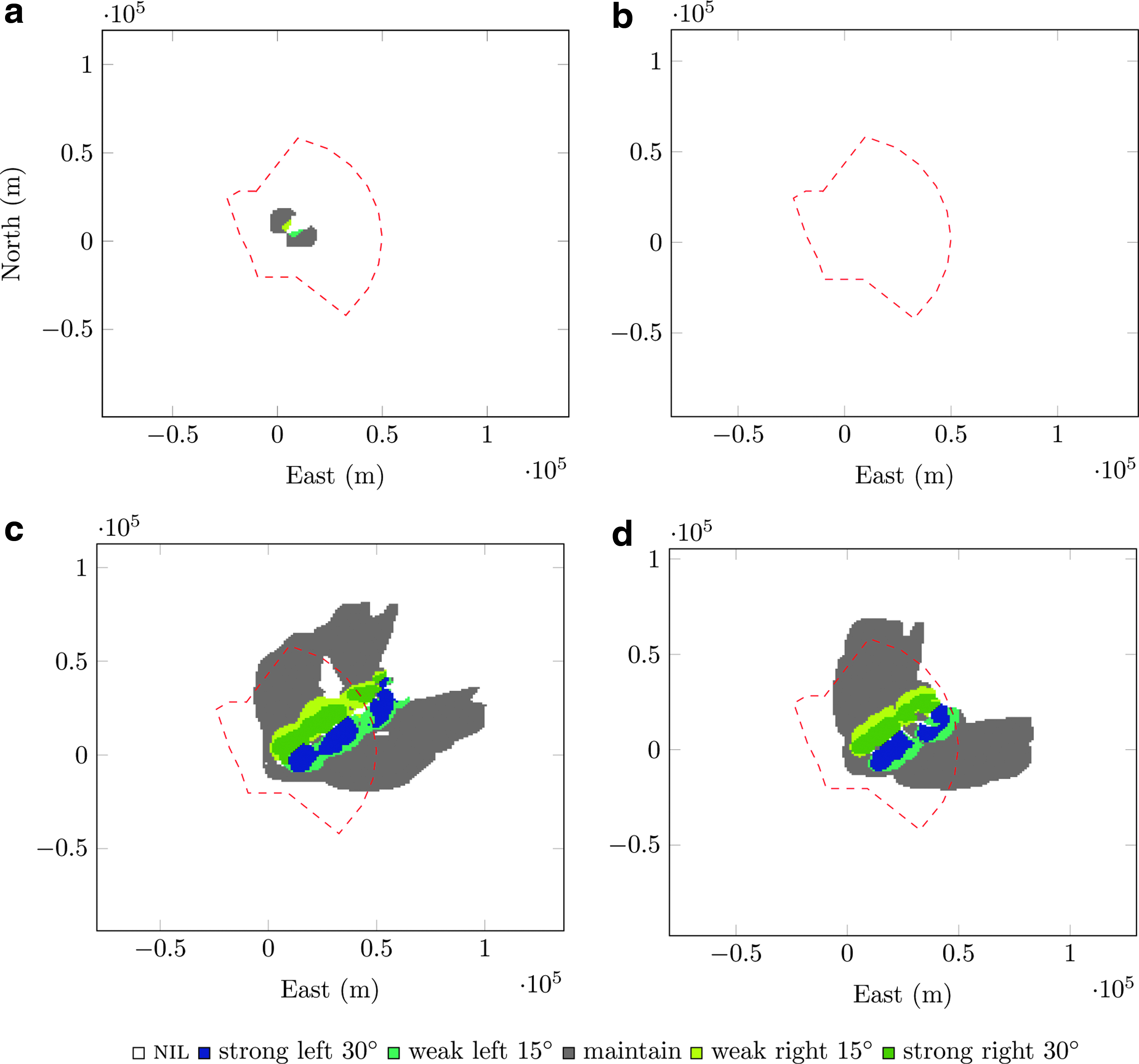
Optimal policy over time. (a) Policy 0 s after launch, (b) 50 s after launch, (c) 250 s after launch, and (d) 400 s after launch.

At 0 s after launch (Fig. 5a), there are minimal reroutes that ensure no aircraft interacts with the commercial space launch vehicle that passes through the airspace at 50 s. Since there is still reaction time, the commanded actions are less disruptive (maintain and weak left or right). At 50 s after launch (Fig. 5b), there is no longer any action to take to avoid the commercial space launch vehicle that is actively passing through the airspace and there is no risk yet of debris.

At 80 s after launch, we model an anomaly and debris starts to propagate toward the airspace. At 250 s after launch (Fig. 5c), there have been, are, and will be pieces of debris falling through the airspace. There are strong maneuvers recommended immediately around where the debris passes through the airspace and less disruptive commands further out. The maintain region extends toward the top right because this model does not know the aircraft's trajectory, just the current heading, and so, it uses the least disruptive (and cheapest) action, maintain, to ensure the aircraft is safe as it gets closer to the debris. A similar pattern occurs 400 s after launch (Fig. 5d).

We integrated the policy into a simulation framework to model how real flights in a launch area would interact with this system. Figure 6 shows an example flight. The blue line represents the flight when there is no launch. The red dashed line represents the flight rerouted with the presented MDP policy. The black outline represents an example prohibited region during a commercial space launch. This plot shows how our method is able to reroute with smaller flight deviations, keeping the airspace as efficient as possible. More detailed results of this technique are presented in Tompa et al.⁹ and Tompa and Kochenderfer.¹⁰

Fig. 6.

Example rerouted MDP rerouted flight.

Future Recommendations

This approach creates real-time reroutes for aircraft during a commercial space launch while ensuring safety and promoting efficiency. The reroutes are all solved before the commercial space launch and can be queried based on the aircraft state and launch vehicle conditions. This approach can also be extended to accommodate additional flight conditions, such as oceanic flights rerouted through metering rather than heading changes. We anticipate that the initial implementation in the airspace would have air traffic controllers querying the policies, informing the pilots of any actions, and managing command updates. In the future, we hope this system could be included on board to automatically inform pilots.

Footnotes

Acknowledgments

This work is sponsored by the FAA Center of Excellence for Commercial Space Transportation Task 331. Opinions, interpretations, conclusions, and recommendations are those of the authors and are not necessarily endorsed by the U.S. Government.

Author Disclosure Statement

No competing financial interests exist.

References

Addressing the challenges to aviation from evolving space transportation. Tech. rep. Washington, DC: Air Line Pilots Association International, 2018.

U.S. passenger carrier delay costs. Tech. rep., Airlines for America, 2018, http://airlines.org/dataset/perminute-cost-of-delays-to-u-s-airlines (Last accessed on January 22, 2019).

FAA. Commercial space transportation forecasts. May 2014. www.faa.gov/about/office_org/headquarters_offices/ast/media/2014_GSO_NGSO_Forecast_Report_FAA_COMSTAC_July_15_2014.pdf (Last accessed on January 22, 2019).

Murray

, VanSuetendael

. A tool for integrating commercial space operations into the National Airspace System. Presented at the AIAA Atmospheric Flight Mechanics Conference and Exhibit, Keystone, CO, August 21-24, 2006.

Colvin

, Alonso

. Compact envelopes and SU-FARM for integrated air-and-space traffic management. Presented at the AIAA Aerospace Sciences Meeting, American Institute of Aeronautics and Astronautics, Kissimmee, FL, January 5-9, 2015.

Bilimoria

, Jastrzebski

. Space transition corridors in the National Airspace System. Presented at the Aviation Technology, Integration, and Operations Conference, Los Angeles, CA, August 12-14, 2013.

Johnson

, Sollenberger

, Schulz

, Yuditsky

, Hatton

“Space vehicle operations debris threat mitigation study. Tech. Rep. DOT/FAA/TC-16/12, Atlantic City, NJ: Federal Aviation Administration, 2016.

Puterman

ML.

Markov Decision Processes: Discrete Stochastic Dynamic Programming. Hoboken, NJ: Wiley, 2005.

Tompa

, Kochenderfer

, Cole

, Kuchar

. Optimal aircraft rerouting during commercial space launches. Presented at the Digital Avionics Systems Conference (DASC), Prague, September 13-17, 2015.

10.

Tompa

, Kochenderfer

. Optimal aircraft rerouting during space launches using adaptive spatial discretization. Presented at the Digital Avionics Systems Conference (DASC), London, England, September 23-27, 2018.

11.

Bilimoria

, Sridhar

, Chatterji

, Sheth

, Grabbe

. FACET: Future ATM concepts evaluation tool. Presented at the USA/Europe Air Traffic Management R&D Seminar, Napoli, Italy, June 13-16, 2000.

12.

Lin

MYY

, Larson

EWF

, Collins

. Determination of debris risk to the public due to the Columbia breakup during reentry. Appendix D.16, September 2003.

13.

Capristan

, Alonso

. Range Safety Assessment Tool (RSAT): An analysis environment for safety assessment of launch and reentry vehicles. Presented at the AIAA Aerospace Sciences Meeting, American Institute of Aeronautics and Astronautics, National Harbor, Maryland, January 6, 2014.

14.

Kochenderfer

Decision Making Under Uncertainty: Theory and Application. Cambridge, MA: MIT Press, 2015.

15.

Kochenderfer

, Chryssanthacopoulos

. Robust airborne collision avoidance through dynamic programming. Project Report ATC-371. Lexington, MA: Massachusetts Institute of Technology, Lincoln Laboratory, January 2011.