Code-Free Machine Learning Solutions for Microscopy Image Processing: Deep Learning

Abstract

In recent years, there has been a significant expansion in the realm of processing microscopy images, thanks to the advent of machine learning techniques. These techniques offer diverse applications for image processing. Currently, numerous methods are used for processing microscopy images in the field of biology, ranging from conventional machine learning algorithms to sophisticated deep learning artificial neural networks with millions of parameters. However, a comprehensive grasp of the intricacies of these methods usually necessitates proficiency in programming and advanced mathematics. In our comprehensive review, we explore various widely used deep learning approaches tailored for the processing of microscopy images. Our emphasis is on algorithms that have gained popularity in the field of biology and have been adapted to cater to users lacking programming expertise. In essence, our target audience comprises biologists interested in exploring the potential of deep learning algorithms, even without programming skills. Throughout the review, we elucidate each algorithm’s fundamental concepts and capabilities without delving into mathematical and programming complexities. Crucially, all the highlighted algorithms are accessible on open platforms without requiring code, and we provide detailed descriptions and links within our review. It’s essential to recognize that addressing each specific problem demands an individualized approach. Consequently, our focus is not on comparing algorithms but on delineating the problems they are adept at solving. In practical scenarios, researchers typically select multiple algorithms suited to their tasks and experimentally determine the most effective one. It is worth noting that microscopy extends beyond the realm of biology; its applications span diverse fields such as geology and material science. Although our review predominantly centers on biomedical applications, the algorithms and principles outlined here are equally applicable to other scientific domains. Furthermore, a number of the proposed solutions can be modified for use in entirely distinct computer vision cases.

Impact Statement

Impact statement In our article, we invite researchers to familiarize themselves with the principles of operation of widely used deep learning algorithms in the analysis of microscopic images and the most convenient and advanced open examples of their no-code application. A significant advantage of our review is that we help our colleagues understand the mechanisms of algorithm operation using simple language, devoid of complex mathematical terms and formulas, without delving into programming intricacies. Thus, a researcher who reads our review will be able to grasp the basic mechanics of the algorithm of interest and find a specific solution without requiring a substantial amount of time to master it.

Introduction

General concept of deep learning, traditional versus deep from the point of deep learning

Deep learning, a subfield of machine learning, draws inspiration from the structure and functioning of biological neural networks, particularly the human brain (see Fig. 1). In this study, information processing occurs through interconnected neurons. Neurons are individual computational units that receive electrical signals (inputs) from thousands of other neurons through their dendrites. These signals are then processed within the neuron, and if a certain threshold is reached, the neuron fires an electrical signal along its axon to communicate with other neurons. The brain as the system with all its complex functions consists of billions of such neurons, and each of them takes signals from other neurons as an input and outputs a response to next neurons. Deep learning mimics this neural structure in a computational setting. Instead of biological neurons, deep learning uses artificial neurons, often called “units” or “nodes.” These artificial neurons are organized into layers within a neural network.

FIG. 1.

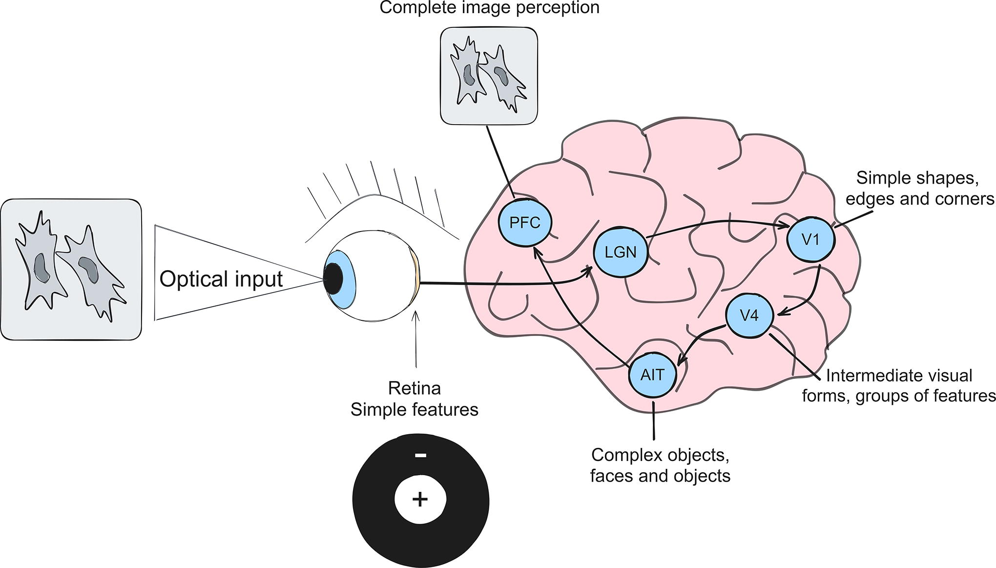
Principle of operation of the visual analyzer. AIT, anterior inferotemporal cortex; LGN, lateral geniculate nucleus; PFC, prefrontal cortices; V1, cortical area V1; V4, cortical area V4.

In addition, similar to its biological prototype, deep learning is based on the idea of hierarchical feature learning. In traditional machine learning, the process of learning is happening after a feature extraction process that is done by a nontrainable human-created pipeline, which is not only demanding for time and work of human professionals but also can be suboptimal for challenging tasks. Despite that, feature extraction by nontrainable pipelines is still actively used in tissue biology studies.^1,2 In contrast, in deep learning feature, extraction is done automatically as it is a trainable part of the algorithm, which allows better grasp on data complexities. Moreover, deep learning allows extracting features of different levels of complexity because of the hierarchical structure of the feature extraction pipeline. In other words, it can extract features from already-extracted features and do so several times in a row. Thus, the process of feature extraction became not only automatic but also more powerful owing to its multilayer structure; thus, deep learning-based feature extraction became popular in tissue biology and tissue engineering studies.^3,4

Some important points of deep learning:

It promotes end-to-end learning, where a model is trained to map raw input data directly to the desired output. This significantly simplifies the modeling process.

Deep learning models, once trained on one task, can often be repurposed for related tasks with minimal adjustments. This is known as transfer learning, and it leverages the hierarchical features learned by the model to tackle new problems.

Such networks can be scaled by increasing the number of layers and neurons, allowing them to learn increasingly complex representations. This scalability is a key factor in their ability to handle large and diverse datasets.

Important concepts and definitions in deep learning

In deep learning, all models are trained with the same principle. The algorithm is initially being created with random (or zeroed) parameters, and in that state, its outputs are also random. Then training data from the dataset are presented to the algorithm, and its parameters are gradually being changed to better represent the data transformation that is happening in the dataset. To achieve better results, hyperparameter values are assigned to the model before training. The following are the most important ones:

Loss function. Similar to what happens in traditional machine learning, loss function is needed to estimate how significantly our model is wrong. A model with randomly initialized parameters has a huge loss, and a model with perfect performance has zero loss. The loss is calculated at the end of the algorithm pass—the model’s outputs are compared with ground truth, and then the process of calculating the loss not only at the end but also from the point of view of every parameter in the model happens (for deep learning models, it is called backpropagation). This will give a direction for each parameter tweak for better performance. Loss function is dependent on the modality of the task—there are distinct loss functions for classification problems, segmentation, object detection, and so on.

Optimizer. The algorithm that changes parameters for better performance is called optimizer. The direction in which we should change each parameter is already known from calculating loss and backpropagation. Optimizer pushes each parameter in that direction with a step size called learning rate and with certain rules specific for the optimizer itself.

Epochs. The process, including model output calculation, loss calculation, loss backpropagation, and updating parameters by optimizer, is called an epoch and repeated several times until the model’s performance is at its best. The number of epochs determines how many times the entire training dataset is used during training. Setting this too low may result in underfitting, whereas setting it too high may lead to overfitting.

Number of layers and units. This refers to the architecture of the neural network, including how many layers it has and how many neurons (or units) are in each layer. This includes specifying the type of layers (e.g., fully connected, convolutional, and recurrent) and their order.

Batch size. This hyperparameter defines the number of training examples used in each iteration of training. It can influence the speed and stability of training.

Activation functions. Activation functions introduce nonlinearity to the model. Common activation functions include Rectified Linear Unit (ReLU), sigmoid, and tanh. Choosing the right activation functions can significantly affect the network’s performance. Adding nonlinearity is very important for modeling complex nonlinear relationships in data. Moreover, the activation function acts as a filter that is activated in response to certain characteristics of the input data. This function allows highlighting important features and suppressing unnecessary ones.

Learning rate schedule. Instead of a fixed learning rate, a schedule can be used to adapt the learning rate during training. Common schedules include step decay, exponential decay, and cyclical learning rates.

Same as in traditional machine learning, after each training epoch, validation data must be transferred to the model. These data must be different from training data and not transferred to training. Thus, we can perform an early stopping-catching at the moment of overfitting (in case it happens) and yield a peak performing model.

Areas of application of deep learning algorithms

Deep learning is used in many areas of computer vision, including biomedical sciences, in general,⁵ and microscopy, in particular. Here are most popular modalities of problems in microscopy that are currently being solved with deep learning (see Fig. 2):

FIG. 2.

Modalities of problems in microscopy that are being solved with deep learning algorithms.

(1)

Image classification, that is, predicting a probability of a whole image belonging to some class.⁶ It is used for different tissue biology tasks, for example, diagnostics of biopsy material.^7–9

(2)

Image segmentation, that is, predicting whether each pixel on an image belongs to some class.¹⁰ There are different segmentation subtypes: semantic, instance, panoptic, and others. Such approaches can be useful in cases where we need to highlight some objects in images. These may be clusters of cells in biological sections, individual cells, or even their compartments. Different deep learning-based segmentation techniques are widely used in cell and tissue assays.¹¹

(3)

Object detection, that is, predicting a possibility of an object of a particular class existing in a certain region of the image.¹² Object detection is actively used in different tissue engineering systems.^13,14

(4)

Image translation, that is, predicting a different image based on an input image.¹⁵ Image translation is used for artificial staining of unlabeled images of cells and tissues^16,17 and for other purposes.¹⁸

(5)

Image restoration, such as denoising or resolution upgrading.¹⁹ These techniques, while being useful for all types of images, are also actively used for tissue biology studies.²⁰

Principle of Convolution—Basis of Deep Learning in Image Processing (and Advent of Transformers)

When it comes to applying deep learning to image processing, it is usually assumed that there is a set of filters with parameters (weights), same as in feature extraction with constant filters for traditional machine learning but only their values are trainable, that is, they are changed during the training process in such a way as to better fit the dataset. The result of applying such filters is feature maps (also same as in feature extraction with constant filters, but only these feature maps contain relevant to specific dataset features) that help extract important characteristics of objects located in images (see Fig. 3A). A set of such filters is called convolutional layer, and neural network architecture based on the sequential application of several such layers is called convolutional neural network (CNN). When processing an image using a CNN, each subsequent convolutional layer extracts increasingly complex and important features by applying its filters to the feature maps from the previous layers (see Fig. 3B). This is the concept of CNNs, in which convolutional layers are stacked one after another to automatically extract increasingly higher-order features. This makes such architectures particularly well suited for tasks like image classification, object detection, image segmentation, and more, although with increase in performance comes a major disadvantage: deep learning models require much more computational powers to run.

FIG. 3.

(A) Visualization of the convolution process using the example of one filter with trainable parameters. (B) The general principle of using convolutional layers in neural networks and using their output in solving further computer vision problems.

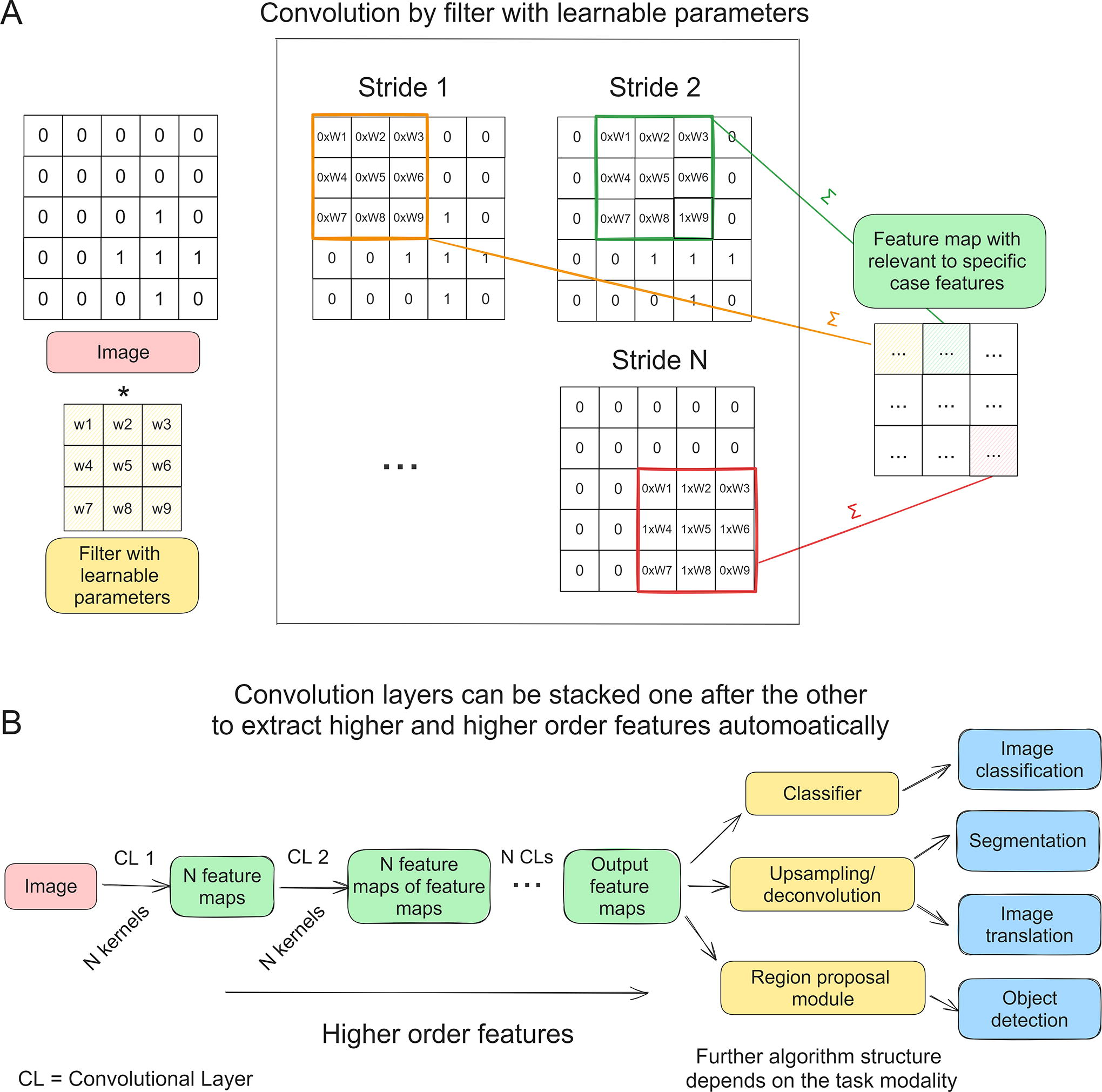
Between convolutional layers, pooling layers are often used to reduce the spatial dimensions of the feature maps. Pooling (e.g., max-pooling or average-pooling) aggregates information from small regions of the feature maps, reducing computational complexity and providing a degree of translation invariance. Nonlinear activation functions, such as ReLU, are applied to the output of each convolutional layer. These functions introduce nonlinearity to the network, enabling it to learn complex relationships in the data.

Currently, in addition to CNN, a different deep learning image processing paradigm emerged—Vision Transformers (ViTs). ViTs extend the Transformer architecture, originally designed for natural language processing tasks like machine translation, to process and analyze visual data, such as images and videos. Although CNNs utilize the principle of kernels with trainable parameters, in ViTs, images are divided into a grid of nonoverlapping patches. Each of them is transformed into a fixed-dimensional vector, which captures both the content and the spatial information of each patch. ViTs consist of multiple Transformer encoder layers stacked on top of each other. Each encoder layer contains a multihead self-attention mechanism followed by feedforward neural networks. Self-attention is a mechanism that allows the model to learn long-range dependencies between the patches.

CNN architectures and ViT models are now often used together because they are complementary: CNNs are good at extracting local features; ViTs are able to analyze global dependencies. Combining them can improve performance in computer vision tasks. Unfortunately, at the moment there are no open code-free resources in which such combined models, or individual ViT models, would be presented. However, it is already obvious that image processing will progress in this direction, which means that appropriate resources will appear.

In summary, the core idea of convolutional networks is to automatically learn hierarchical features from grid-like data by applying convolutional operations and gradually increasing the abstraction of learned features. This hierarchical algorithm structure is a major CNN advantage for difficult tissue biology tasks.²¹ But a stack of convolutional layers is only a basis of deep learning models for image processing, as it provides feature maps that should be further processed by a consequent algorithm. The structure of such an algorithm depends on task modality (see Fig. 3B). For an image classification task, output feature maps get flattened into a feature vector and then processed by a classifier; or, in case of segmentation, a set of output feature maps gets upsampled back into a binary layer. The next sections present a brief description of deep learning models for different image processing tasks with references to where they can be implemented in a code-free manner.

Deep Learning Algorithms: Inner Mechanics of Algorithms for Each Task

Deep learning for image classification

The most popular approach to image classification is flattening feature maps produced by convolutional layers into a vector and then processing it by some classifier. Often the classifier is fully connected neural network (FCNN, also referred to as dense neural network), which is a structure that consists of neurons arranged in layers, and each neuron in a layer is connected with each neuron in the previous layer (see Fig. 4). This structure is the most popular tool for image classification in general, including microscopy image processing in particular.^22,23 It is important to note that the aforementioned traditional machine learning methods can be successfully used instead of FCNN.²⁴

FIG. 4.

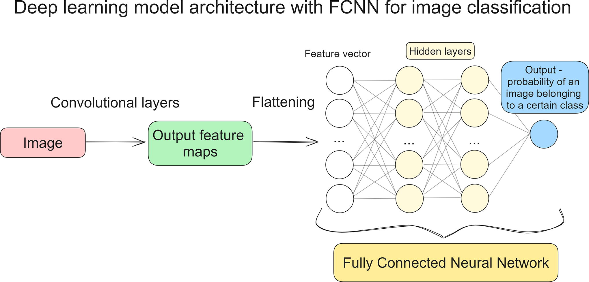
One of the most popular deep learning algorithm structures for image classification-fully connected layers following convolutional ones. Instead of FCNN, traditional machine learning classifiers can be used, for example, random forest or boosting algorithms. FCNN, fully connected neural network.

As discussed earlier, Orange^25,26 presents tools for image classification with pretrained neural network for image embedding and then applying some classifier (options include FCNN). The main advantage of this approach is that there is no need for a large amount of computational power and time for model training as all deep learning parts are already pretrained and run on a remote machine; in contrast, this can lead to suboptimal performance on datasets where features to extract are too specific for pretrained models to grasp. To our best knowledge, the only code-free alternative to Orange for image classification is Microscopic Image Analyzer (MIA)²⁷ with a vast model backbone selection, image preprocessing and augmentations, and hyperparameter tuning options for training a model on a custom dataset, although it requires accordingly computational resources (GPU [graphics processing unit] performance and memory being most necessary).

Segmentation models

Segmentation models are a category of neural networks used in computer vision and image processing tasks to identify and classify objects or regions of interest within an image. They are particularly useful in the field of microscopy image processing, where precise delineation of structures, cells, or particles is essential.

Segmentation models can be broadly categorized into two types: semantic segmentation and instance segmentation.

Semantic segmentation

Semantic segmentation involves labeling each pixel in an image with a corresponding class label, typically representing the type of object or material it belongs to. This type of segmentation is used when the goal is to classify regions without distinguishing individual instances. For example, in a microscopy image of tissue samples, semantic segmentation can be used to differentiate between different cell types or tissue structures.

Semantic segmentation models consist of blocks of convolution and max-pooling layers (downsampling path/encoder) and deconvolution layers (upsampling path/decoder). Encoder allows to get important features, and max-pooling layers help to strengthen and save them, allowing to get rid of information that is not essential for the success of the algorithm. Although encoder reduces dimensions of input image by applying consequent convolutions, decoder returns the image to its original dimensions by applying an operation opposite to convolution. Instead of a regular kernel, it uses a transposed kernel, which is essentially a flipped and stretched version of the original filter used in the convolution, with trainable weights. In order to recover fine-grained spatial information that is lost during downsampling, skip connections are used.

One of the most popular architectures for semantic segmentation is U-net. In it, convolutional layers (encoder) produce final feature maps that are further processed by trainable upsampling layers (decoder) to a binary layer. For saving information discovered by first convolutional layers, skip connections are created to connect feature maps produced by them to corresponding upsampled feature maps (see Fig. 5). U-net thus achieves a fully trainable symmetrical image-to-binary pipeline. U-net for semantic segmentation can be trained on custom dataset in ImageJ U-net plugin, DeepMIB, and ZeroCostDL4Mic; pretrained U-nets are available at Bioimage.io.

FIG. 5.

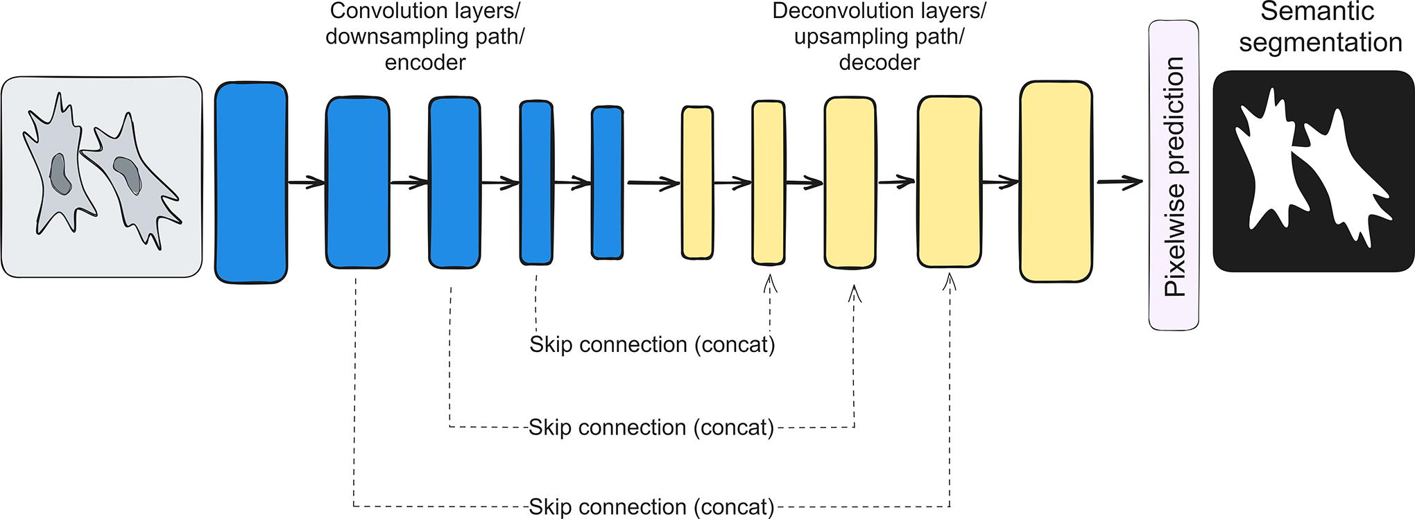
U-net architecture structure.

In microscopy image processing, semantic segmentation models are used to solve such tasks as cell counting,²⁸ tissue segmentation,²⁹ and the identification of specific cellular structures.³⁰

Instance segmentation

The problem with the semantic segmentation strategy is that it is not optimal for counting particles that are overlapping as its loss function optimizes poorly for that (see Fig. 6). There are few methods of correcting this, for example, creating an additional class with an object’s borders. Instance segmentation goes a step further by not only labeling pixels with class information but also distinguishing individual instances of the same class. In microscopy images, this can be particularly valuable when studying complex biological samples containing multiple cells or particles of the same type.

FIG. 6.

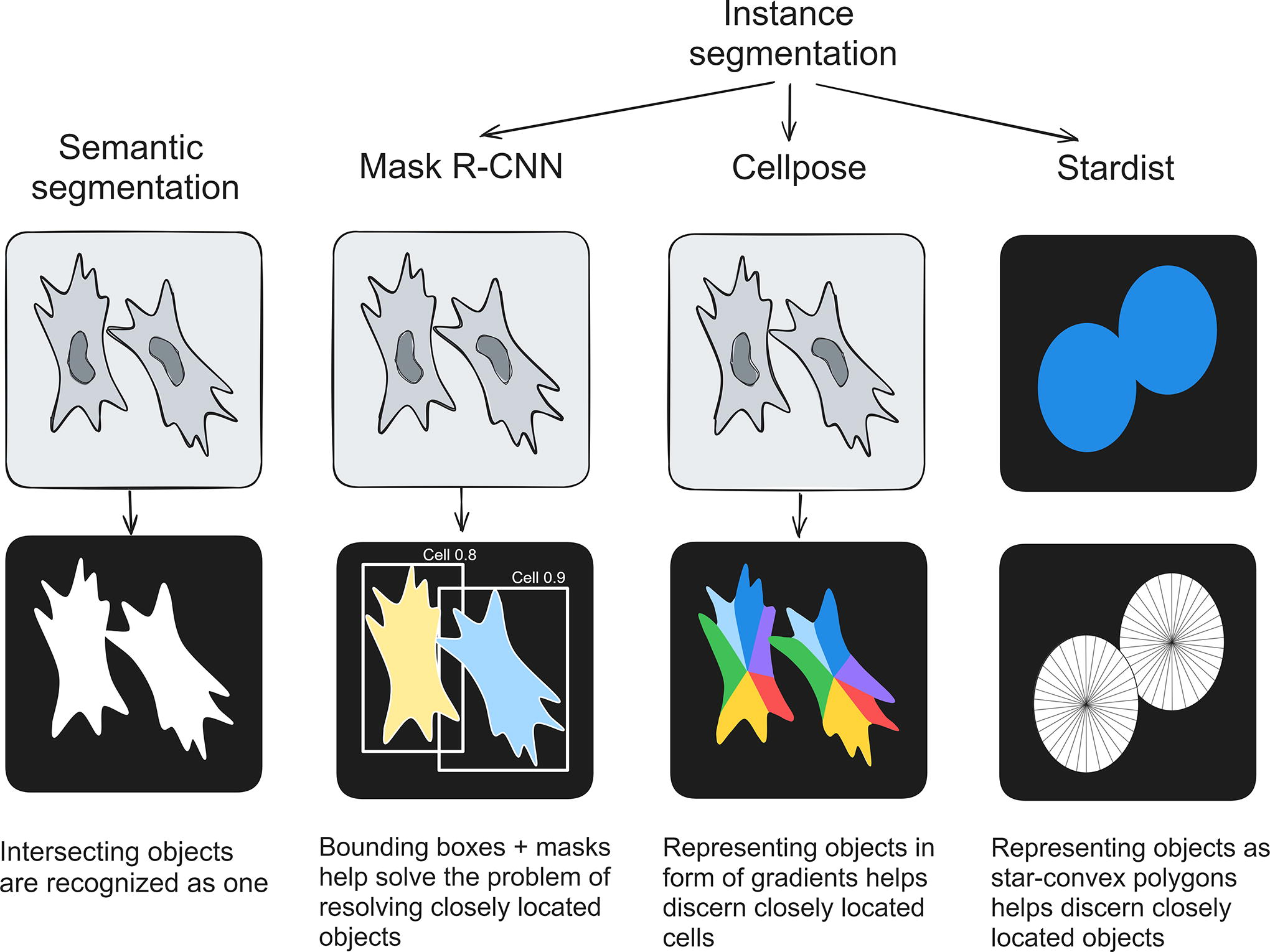
The main idea of semantic and instance segmentation. Examples of instance segmentation approaches. Mask R-CNN, mask region-based convolutional neural network.

Basic instance segmentation models are based on object detection models. The principle of object detection is finding objects on an image with the assignment of bounding box coordinates, as well as the probability of each of them belonging to a particular class. In this case, the binary mask of the object is not predicted; therefore, there is no possibility of extracting its additional properties. The instance segmentation principle additionally involves predicting the mask of each detected object. This approach allows you to segment overlapping objects much more efficiently.

The most frequently used architectures for instance segmentation are as follows:

Mask region-based CNN (Mask R-CNN). It is a deep learning architecture for instance segmentation and object detection tasks. Mask R-CNN builds upon the Faster R-CNN object detection framework by adding a pixel-level segmentation branch, allowing it to simultaneously provide instance masks in addition to bounding box predictions (see Fig. 7).

Mask R-CNN combines three key components as follows:

Region Proposal Network generates region proposals, which are regions of interest in the image that might contain objects. These proposals are used as candidates for both object detection and segmentation.

Object Detection module outputs bounding boxes with precise location of the object within each region proposal and the class probabilities.

Mask generation module drives the network to generate accurate instance masks.

Mask R-CNN has significantly improved the accuracy and efficiency of segmentation of overlapping/closely seeded objects, making it a crucial tool in computer vision and related fields.^31,32 Its ability to provide pixel-level masks for each object instance has opened up new possibilities for precise and detailed image analysis. Training Mask R-CNN on a custom dataset is currently on beta test at ZeroCostDL4Mic.

Microscopy/cell-specific architectures—CellPose and StarDist. Some developers specifically for microscopy purposes modified the output of segmentation models to produce not just binary masks but also some objects that better represent individual cells for improvement in detection and separation (see Fig. 6).

The first example of such architecture is Cellpose, a cell and nucleus segmentation algorithm. Cellpose models produce as an output and not as a binary layer, but gradient maps get processed further to calculate distinct objects on an image;³³ in other words, these models are specifically designed to output representations of cells to better segment them between each other with the main area of application being cells with irregular shape and several protruding processes. Different retrained Cellpose models can be found at Bioimage.io and as Napari plugin; training a Cellpose model on a custom dataset (became available with Cellpose 2.0³⁴) is available at ZeroCostDL4Mic and in Cellpose own graphical user interface (GUI).

Another biology-specific approach is StarDist,³⁵ a set of instance segmentation models based on representing objects as star–convex polygons (shapes where all perimeter points can be connected to the center of the object with a straight line). This approach is especially relevant for segmenting nuclei, as star–convex polygons are an excellent representation of them. Pretrained StarDist models can be found at Bioimage.io or as a Napari plugin, and training on a custom dataset is available at ZeroCostDL4Mic.

FIG. 7.

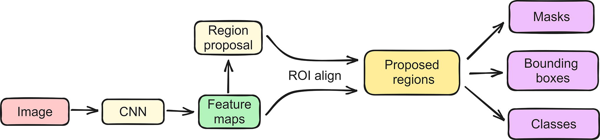
Mask R-CNN architecture structure. Mask R-CNN, mask region-based convolutional neural network; ROI, a region of interest.

Image translation models

As in segmentation, feature maps produced by a stack of convolutional layers can be upsampled but not into a binary layer but in an image. Thus, such a model would take an image as an input and produce a different image as an output; for example, it would take a brightfield image and transform it into a fluorescent one, thereby allowing reduction in dye expenses or timelapse visualization of processes without impact from fluorescent dyes. Image-to-image transition is especially relevant in microscopy as it’s relatively easy to create a dataset with paired images taken in different channels without labor-intensive annotations.³⁶

There are several approaches to image-to-image transitions, but among them the code-free options are available only for Cycle Generative Adversarial Network (CycleGAN) and pix2pix GAN, both in the ZeroCostDL4Mic framework. GANs consist of two algorithms: generator (does convolution and upsampling—the main part of a model) and discriminator (classifier that discerns ground truth and generated images). During training, the discriminator learns to classify between generated images and ground truth, whereas the generator learns to deceive the discriminator. Such a peculiar training process allows for better performance of the generator.

CycleGAN and pix2pix GAN operate similarly; the main difference lies in the dataset format (see Fig. 8):

FIG. 8.

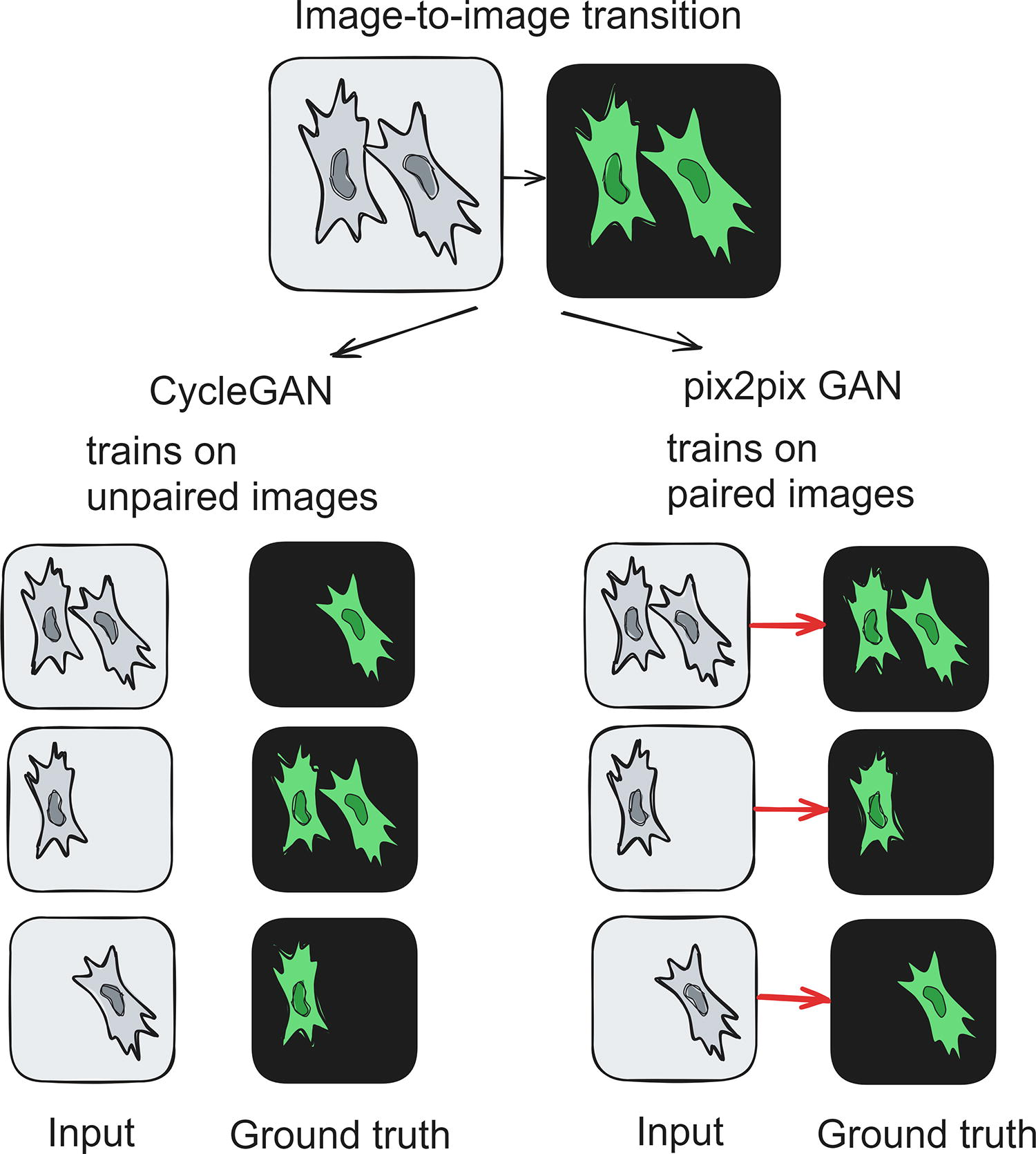
Two main approaches to image-to-image translation, CycleGAN and pix2pix GAN. CycleGAN can be trained on the dataset that consists of unpaired images, whereas pix2pix GAN is trained on paired images. CycleGAN, Cycle Generative Adversarial Network.

CycleGAN is trained on datasets with unpaired images (just sets of input and output images not necessarily of the same fields of view and without internal link between each other).

pix2pix is trained on datasets with paired images (pairs of images of the same field of view in different microscopy modalities).

Image-to-image models are used both for conversion of brightfield images to both histological³⁷ and fluorescent³⁸ staining images. Both CycleGAN and pix2pix GAN are available to train on the custom datasets in ZeroCostDL4Mic Google Colab notebooks.

Image restoration and resolution upsampling models

In microscopy upgrading the quality of an image is an especially widespread problem as often it is impossible to obtain a perfect image without noise or with super resolution because of technical restraints. Many traditional methods of image restoration exist,³⁹ but several machine-learning based approaches emerged with better performance.⁴⁰ The main idea is image-to-image translation, same as in CycleGAN or pix2pix GAN, but without major modality shift and with removing the noise or changing resolution.

There are several strategies to image restoration in terms of dataset structure. There are models with supervised training, which means that dataset is input and ground truth images (see CARE models at ZeroCostDL4Mic); models with self-supervised learning, which means that the dataset is only noisy or low-quality images and model figures out denoising or resolution upgrading steps on itself (see Noise2Void⁴¹ Napari plugin, https://www.napari-hub.org/plugins/napari-n2v, and Noise2Void models at ZeroCostDL4Mic); and models with semisupervised learning, where both labeled and unlabeled images are used for training. Currently image restoration or resolution upsampling models can be utilized in the form of Napari plugins, trained on custom dataset in ZeroCostDL4Mic framework, and several pretrained models can be found at Bioimage.io.

Code-Free Frameworks with Deep Learning Algorithms for Image Processing

Cellpose GUI and Scellseg GUI

Cellpose is an instance segmentation architecture specifically designed for segmenting irregularly shaped and/or closely seeded cells, making it highly relevant for challenging microscopy cases.

Based on the U-net, Cellpose^33,34 main idea is representing objects as gradient maps to discern closely located entities (see Fig. 6). It supports multichannel input images, accommodating various staining techniques. Notably, Cellpose can perform separate nuclear and cytoplasmic segmentation, distinguishing between these components. User-friendly and flexible, Cellpose offers a GUI for easy image loading, segmentation parameter adjustment, and result visualization without coding. It supports batch processing for simultaneous analysis of multiple images and efficiently handles large images using GPU acceleration.

Scellseg,⁴² a Cellpose-based project, enhances the original tool with additional capabilities and an improved GUI. The enhancements include extended annotation features and additional model selection and fine-tuning options, as detailed on the project’s GitHub page.

Napari plugins

Napari is a Python-based multidimensional image viewing and processing software⁴³ with the main concept of it being the basis and user should find and utilize needed functions in form of open-source plugins. Among those several used deep learning algorithms, in particular, Cellpose, StarDist, and Noise2Void plugins can be found as Napari plugins, and the collection of plugins constantly grows.

DeepMIB

Microscopy Image Browser (MIB) is a software for image processing made by a team from the University of Helsinki.⁴⁴ DeepMIB is a module in this software with extensive semantic segmentation capabilities, including training a model on a custom dataset with vast hyperparameter tuning options, training process and test result visualization capabilities, and even possibilities to inspect a trained model’s performance by visualizing processing results of each layer.⁴⁵ Available backbones for semantic segmentation include U-net, DeepLabv3 ResNet18, ResNet50, Xception, and Inception-ResNet-v2. Easy-to-understand video guidelines can be found at the project’s website (http://mib.helsinki.fi/tutorials_segmentation.html).

Pretrained models from Bioimage.io and platforms for them: DeepImageJ and Ilastik

Bioimage.io is a platform with a wide range of pretrained models for biological tasks through open-source, ready-to-use deep learning networks, including various segmentation, generative (virtual staining and resolution-enhancing), and restoration models. But bioimage.io is rather a distributor, whereas there are two main frameworks where one can apply these models, DeepImageJ and Ilastik. DeepImageJ⁴⁶ is another easy-to-install ImageJ plugin that allows examination of available models, installation, and inference with models presented at Bioimage.io. Ilastik is an open-source Python-based software; it is not only a traditional machine learning tools-hosting platform, but it can also be used to run pretrained deep learning models from Bioimage.io. Currently Bioimage.io lists some other supported platforms besides DeepImageJ and Ilastik, such as QuPath or Icy, but only a few models are currently available to run on them.

ImageJ U-net plugin

Another ImageJ plugin is called U-net plugin.⁴⁷ It is based on Caffe deep learning library and allows inference with U-net-based segmentation and object detection models, as well as training on custom data with extensive hyperparameter tuning, validation, and training process visualization capabilities. Its main disadvantage is that it runs only on the Ubuntu operating system or requires a connection to the backend server with Ubuntu.

ZeroCostDL4Mic

ZeroCostDL4Mic⁴⁸ is a collection of ready-to-use, without code writing, remote Google Colab notebooks for deep learning model training and inference. Google Colab is a notebook-based Python environment with remote connection to Google servers and possibilities to use free GPU for running code. ZeroCostDL4Mic presents a set of such notebooks with already-written TensorFlow-based (deep learning Python library) code and instructions on how to use it; only the dataset and desired set of parameters for training are needed from the user. Each notebook comes with extensive step-by-step instructions. There are notebooks for the following: (1)

Segmentation, both semantic and instance. Models available for training and inference are U-net, Mask R-CNN, Cellpose, StarDist, and others.

(2)

Object detection: YOLOv2, Detectron2, and RetinaNet models.

(3)

Different image restoration (denoising) and super-resolution models.

(4)

Image-to-image translation models.

The great advantage of this framework is that it can run remotely on a fast GPU, thus removing the need for expensive hardware being installed locally. However, it requires some basic understanding of how Google Colab notebooks work, and free GPU is available only for a limited amount of time there.

MIA

MIA²⁷ toolkit is a relatively recent Python-based software with a wide variety of deep learning capabilities, including image classification, segmentation, and object detection. The prominent feature of MIA is freedom in constructing a model to train with capabilities to try different backbones for a model, among which there are almost every modern backbone, including a whole variety ranging from light and fast ones to large but slow ones. In addition, MIA includes a remarkable range of options of hyperparameter tuning: users can set up class weights, pick an optimizer and loss function, or set a learning schedule. Another important feature of MIA is extensive image augmentation capabilities, which can increase the model’s accuracy and decrease the chance of overfitting. With that variety of model training, validation, and inference options, MIA is also equipped with a toolset for image annotation and a particle tracking section for postprocessing the results of a deep learning model inference. Overall, it is an extremely powerful tool with a lot of capabilities and a wide range of different settings to tune for case-specific obstacles.

Discussion and Conclusions

Generally, deep learning methods offer remarkable capabilities for microscopic image analysis, especially in tasks that demand high accuracy and automatic feature learning. However, the challenges related to data dependency, computational intensity, interpretability, and expertise required should be carefully considered when choosing deep learning approaches for specific microscopy applications.

The combination of microscopy and machine learning has opened new frontiers in image processing, revolutionizing the way biologists analyze and interpret data. However, a significant challenge arises when we consider that the majority of machine learning applications are embedded within code-based frameworks. This poses a potential difficulty for biologists who may not be proficient in programming. In response to this challenge, there is a growing array of solutions that require minimal or no programming knowledge, intended for a broader audience of researchers. These solutions show a range of image processing modalities in deep learning and are presented in various formats, including plugins integrated into existing software and stand-alone applications (see Table 1).

Table 1.

Summary of Code-Free Frameworks with Deep Learning for Microscopic Image Processing and Their Capabilities

	Image classification	Semantic segmentation	Instance segmentation	Object detection	Image translation	Image restoration
Napari plugins			+			+
Cellpose GUI/Scellseg GUI			+
DeepMIB		+
Pretrained Bioimage.io models		+	+			+
ImageJ U-net plugin		+		+
ZeroCostDL4Mic		+	+	+	+	+
MIA	+	+		+

GUI, graphical user interface; MIA, Microscopic Image Analyzer.

Footnotes

Acknowledgment

This work has been supported by Lomonosov Moscow State University funding: project “Molecular and cellular mechanisms of regenerative processes regulation”.

Authors’ Contributions

E.C.: Conceptualization; Writing—original draft; Writing—reviewing and editing; and Visualization. N.V.: Conceptualization; Writing—original draft; Writing—reviewing and editing; and Visualization. K.K.: Writing—reviewing and editing and Project administration. P.T.-K.: Writing—reviewing and Editing and Project administration.

Disclosure Statement

The authors declare that they have no known competing financial interests or personal relationships that could have appeared to influence the work reported in this article.

Funding Information

This work was supported by Russian Science Foundation grant #19–75-30007 ().

References

Wills

, Robertson

, Summers

, et al. Image-based cell profiling enables quantitative tissue microscopy in gastroenterology. Cytometry A, 2020; 97(12):1222–1237; doi: 10.1002/cyto.a.24042

Sheneman

, Stephanopoulos

, Vasdekis

. Deep learning classification of lipid droplets in quantitative phase images. PLoS One, 2021; 16(4):e0249196; doi: 10.1371/journal.pone.0249196

, Chan

, Ong

, et al. Deep learning for fabrication and maturation of 3D bioprinted tissues and organs. Virtual and Physical Prototyping, 2020; 15(3):340–358; doi: 10.1080/17452759.2020.1771741

Strobel

, Schultz

, Moss

, et al. Quantifying vascular density in tissue engineered constructs using machine learning. Front Physiol, 2021; 12:650714; doi: 10.3389/fphys.2021.650714

Wang

, Zhu

, Wang

S-H

, et al. A review of deep learning on medical image analysis. Mobile Netw Appl, 2021; 26(1):351–380; doi: 10.1007/s11036-020-01672-7

Wang

, Fan

, Wang

. Comparative analysis of image classification algorithms based on traditional machine learning and deep learning. Pattern Recognition Letters, 2021; 141:61–67; doi: 10.1016/j.patrec.2020.07.042

Yousif

, Van Diest

, Laurinavicius

, et al. Artificial intelligence applied to breast pathology. Virchows Arch, 2022; 480(1):191–209; doi: 10.1007/s00428-021-03213-3

Sultan

, Elgharib

, Tavares

, et al. The use of artificial intelligence, machine learning and deep learning in oncologic histopathology. J Oral Pathol Med, 2020; 49(9):849–856; doi: 10.1111/jop.13042

Zheng

, Jiang

, Xie

, et al. Feature extraction from histopathological images based on nucleus-guided convolutional neural network for breast lesion classification. Pattern Recognition, 2017; 71:14–25; doi: 10.1016/j.patcog.2017.05.010

10.

Ghosh

, Das

, et al. Understanding deep learning techniques for image segmentation. ACM Comput Surv, 2019; 52(4):1–35; doi: 10.1145/3329784

11.

Greenwald

, Miller

, Moen

, et al. Whole-cell segmentation of tissue images with human-level performance using large-scale data annotation and deep learning. Nat Biotechnol, 2022; 40(4):555–565; doi: 10.1038/s41587-021-01094-0

12.

Dhillon

, Verma

. Convolutional neural network: A review of models, methodologies and applications to object detection. Prog Artif Intell, 2020; 9(2):85–112.

13.

, Wang

, Shi

, et al. Automated contact assembly of vessel-mimetic microstructure through position and orientation estimation based on object detection. In 2017 IEEE International Conference on Robotics and Biomimetics (ROBIO) IEEE: Macau; 2017; pp. 1118–1123; doi: 10.1109/ROBIO.2017.8324567

14.

Yang

, Martin

, Brouillette

, et al. Objective evaluation of chondrocyte density & cloning after joint injury using convolutional neural networks. J Orthop Res, 2022; 40(11):2609–2619; doi: 10.1002/jor.25295

15.

Alotaibi

. Deep generative adversarial networks for image-to-image translation: A review. Symmetry, 2020; 12(10):1705; doi: 10.3390/sym12101705

16.

Christiansen

, Yang

, Ando

, et al. In silico labeling: Predicting fluorescent labels in unlabeled images. Cell, 2018; 173(3):792–803.e19; doi: 10.1016/j.cell.2018.03.040

17.

Rivenson

, Wang

, Wei

, et al. Virtual histological staining of unlabelled tissue-autofluorescence images via deep learning. Nat Biomed Eng, 2019; 3(6):466–477; doi: 10.1038/s41551-019-0362-y

18.

Rozo

, Miskovic

, Rose

, et al. A deep learning image-to-image translation approach for a more accessible estimator of the healing time of burns. IEEE Trans Biomed Eng, 2023; 70(10):2886–2894; doi: 10.1109/TBME.2023.3267600

19.

Wali

, Naseer

, Tamoor

, et al. Recent progress in digital image restoration techniques: A review. Digital Signal Processing, 2023; 141:104187; doi: 10.1016/j.dsp.2023.104187

20.

Xiao

, Fang

, Zhu

, et al. Deep learning-enabled efficient image restoration for 3D microscopy of turbid biological specimens. Opt Express, 2020; 28(20):30234–30247; doi: 10.1364/OE.399542

21.

Geng

, Zhang

, Prabhu

, et al. 3D microscopy and deep learning reveal the heterogeneity of crown-like structure microenvironments in intact adipose tissue. Sci Adv, 2021; 7(8):eabe2480; doi: 10.1126/sciadv.abe2480

22.

Wahid

, Ahmed

, Habib

. Classification of microscopic images of bacteria using deep convolutional neural network. In: 2018 10th International Conference on Electrical and Computer Engineering (ICECE) IEEE: Dhaka, Bangladesh; 2018; pp. 217–220; doi: 10.1109/ICECE.2018.8636750

23.

Wang

, Chen

, Yang

, et al. Classification of mice hepatic granuloma microscopic images based on a deep convolutional neural network. Appl Soft Comput, 2019; 74:40–50; doi: 10.1016/j.asoc.2018.10.006

24.

Ramaneswaran

, Srinivasan

, Vincent

PMDR

, et al. Hybrid inception v3 XGBoost model for acute lymphoblastic leukemia classification. Computat Math Methods Med, 2021; 2021:1–10; doi: 10.1155/2021/2577375

25.

Demšar

, Curk

, Erjavec

, et al. Orange: Data mining toolbox in Python. J Mach Learn Res, 2013; 14(1):2349–2353.

26.

Godec

, Pančur

, Ilenič

, et al. Democratized image analytics by visual programming through integration of deep models and small-scale machine learning. Nat Commun, 2019; 10(1):4551; doi: 10.1038/s41467-019-12397-x

27.

Körber

. MIA is an open-source standalone deep learning application for microscopic image analysis. Cell Rep Methods, 2023; 3(7):100517; doi: 10.1016/j.crmeth.2023.100517

28.

Kong

, Li

, Ren

, et al. Automated yeast cells segmentation and counting using a parallel U-Net based two-stage framework. OSA Contin, 2020; 3(4):982; doi: 10.1364/OSAC.388082

29.

Oskal

KRJ

, Risdal

, Janssen

EAM

, et al. A U-net based approach to epidermal tissue segmentation in whole slide histopathological images. SN Appl Sci, 2019; 1(7):672; doi: 10.1007/s42452-019-0694-y

30.

Punn

, Agarwal

. Inception u-net architecture for semantic segmentation to identify nuclei in microscopy cell images. ACM Trans Multimedia Comput Commun Appl, 2020; 16(1):1–15; doi: 10.1145/3376922

31.

Fujita

, Han

X-H

. Cell Detection and Segmentation in Microscopy Images with Improved Mask R-CNN. In: Computer Vision – ACCV 2020 Workshops. ACCV 2020. Lecture Notes in Computer Science, Vol.12628( Sato

, Han

. eds.). Springer, Cham; 2020.

32.

Dhieb

, Ghazzai

, Besbes

, et al. An automated blood cells counting and classification framework using mask R-CNN deep learning model. In: 2019 31st International Conference on Microelectronics (ICM); 2019; pp. 300–303.

33.

Stringer

, Wang

, Michaelos

, et al. Cellpose: A generalist algorithm for cellular segmentation. Nat Methods, 2021; 18(1):100–106; doi: 10.1038/s41592-020-01018-x

34.

Pachitariu

, Stringer

. Cellpose 2.0: How to train your own model. Nat Methods, 2022; 19(12):1634–1641; doi: 10.1038/s41592-022-01663-4

35.

Schmidt

, Weigert

, Broaddus

, et al. Cell detection with star-convex polygons. 2018; doi: 10.48550/ARXIV.1806.03535

36.

Kreiss

, Jiang

, Li

, et al. Digital staining in optical microscopy using deep learning – A review. 2023; doi: 10.48550/ARXIV.2303.08140

37.

Rivenson

, Liu

, Wei

, et al. PhaseStain: The digital staining of label-free quantitative phase microscopy images using deep learning. Light Sci Appl, 2019; 8(1):23; doi: 10.1038/s41377-019-0129-y

38.

Lee

, Oh

J-W

, Her

N-G

, et al. DeepHCS + +: Bright-field to fluorescence microscopy image conversion using multi-task learning with adversarial losses for label-free high-content screening. Med Image Anal, 2021; 70:101995; doi: 10.1016/j.media.2021.101995

39.

Fan

, Zhang

, Fan

, et al. Brief review of image denoising techniques. Vis Comput Ind Biomed Art, 2019; 2(1):7; doi: 10.1186/s42492-019-0016-7

40.

Tian

, Fei

, Zheng

, et al. Deep learning on image denoising: An overview. Neural Netw, 2020; 131:251–275; doi: 10.1016/j.neunet.2020.07.025

41.

Krull

, Buchholz

T-O

, Jug

. Noise2Void—Learning denoising from single noisy images. In: 2019 IEEE/CVF Conference on Computer Vision and Pattern Recognition (CVPR) IEEE: Long Beach, CA, USA; 2019; pp. 2124–2132; doi: 10.1109/CVPR.2019.00223

42.

Xun

, Chen

, Zhou

, et al. Scellseg: A style-aware deep learning tool for adaptive cell instance segmentation by contrastive fine-tuning. iScience, 2022; 25(12):105506; doi: 10.1016/j.isci.2022.105506

43.

Ahlers

, Althviz Moré

, Amsalem

, et al. Napari: A multi-dimensional image viewer for python. 2023; doi: 10.5281/ZENODO.3555620

44.

Belevich

, Joensuu

, Kumar

, et al. Microscopy image browser: A platform for segmentation and analysis of multidimensional datasets. PLoS Biol, 2016; 14(1):e1002340; doi: 10.1371/journal.pbio.1002340

45.

Belevich

, Jokitalo

. DeepMIB: User-friendly and open-source software for training of deep learning network for biological image segmentation. PLoS Comput Biol, 2021; 17(3):e1008374; doi: 10.1371/journal.pcbi.1008374

46.

Gómez-de-Mariscal

, García-López-de-Haro

, Ouyang

, et al. DeepImageJ: A user-friendly environment to run deep learning models in ImageJ. Nat Methods, 2021; 18(10):1192–1195; doi: 10.1038/s41592-021-01262-9

47.

Falk

, Mai

, Bensch

, et al. U-Net: Deep learning for cell counting, detection, and morphometry. Nat Methods, 2019; 16(1):67–70; doi: 10.1038/s41592-018-0261-2

48.

Von Chamier

, Laine

, Jukkala

, et al. Democratising deep learning for microscopy with ZeroCostDL4Mic. Nat Commun, 2021; 12(1):2276; doi: 10.1038/s41467-021-22518-0