Identification of Environmental Covariates of West Nile Virus Vector Mosquito Population Abundance

Abstract

The rapid spread of West Nile virus (WNv) in North America is a major public health concern. Culex pipiens–restuans is the principle mosquito vector of WNv in the northeastern United States while Aedes vexans is an important bridge vector of the virus in this region. Vector mosquito abundance is directly dependent on physical environmental factors that provide mosquito habitats. The objective of this research is to determine landscape elements that explain the population abundance and distribution of WNv vector mosquitoes using stepwise linear regression. We developed a novel approach for examining a large set of landscape variables based on a land use and land cover classification by selecting variables in stages to minimize multicollinearity. We also investigated the distance at which landscape elements influence abundance of vector populations using buffer distances of 200, 400, and 1000 m. Results show landscape effects have a significant impact on Cx. pipiens–estuans population distribution while the effects of landscape features are less important for prediction of Ae. vexans population distributions. Cx. pipiens–restuans population abundance is positively correlated with human population density, housing unit density, and urban land use and land cover classes and negatively correlated with age of dwellings and amount of forested land.

Introduction

W est Nile virus (WNv) is an arbovirus, or arthropod-borne virus, that is principally transmitted to humans through the bite of an infected mosquito. The distribution and abundance of vector species is directly dependent on the landscape elements needed for their survival. Each species prefers a certain habitat and accordingly thrives in different landscapes with features essential to its life history. Determination of specific landscape factors associated with vector species will assist in maximizing information obtained from costly mosquito trapping programs, facilitating control efforts, and reducing transmission risk to humans.

WNv is maintained in nature through a bird-mosquito cycle usually involving ornithophilic Culex species mosquitoes and a variety of avian reservoir hosts (Turell et al. 2000, 2005). Virus transmission to humans is not a part of the natural maintenance cycle, and disease in humans is incidental. The most important vector of WNv in the northeastern United States thus far is Culex pipiens, a mosquito with an affinity for human settlements that prefers stagnant water for larval habitats (Turell et al. 2000, 2005, Kilpatrick et al. 2005 ). Culex restuans is also a competent vector of WNv and is almost indistinguishable from Cx. pipiens as adults (DeGaetano 2005, Diuk-Wasser et al. 2006). The two species are often grouped into the Culex pipiens–restuans complex (DeGaetano 2005, Kilpatrick et al. 2005, White et al. 2006, Trawinski and Mackay 2008, 2009). Aedes vexans is a persistent human biter and a possible bridge vector of WNv between birds and mammals (Andreadis et al. 2004). Cx. pipiens–restuans has a flight range of 2 km but usually stays within 200 m of the area of larval emergence. Ae. vexans will travel great distances to find appropriate habitats and has a flight range greater than 25 km (Turell et al. 2005). Cx. pipiens–restuans prefers to lay its eggs in artificial water containers. Ae. vexans is an important floodwater mosquito that prefers temporary pools of water (Hayes et al. 1985, Pratt and Moore 1993). Many techniques have been used to identify mosquito breeding sites, determine habitat quality, and predict vector abundance using landscape features, including correlation (Barnes and Cibula 1979, Hayes et al. 1985, Maupin et al. 1991), overlay (Wagner et al. 1979), discriminant analysis (Wood et al. 1991, 1992, Hugh-Jones et al. 1992), analysis of variance (Pope et al. 1992, 1994, Dister et al. 1997), linear regression (Beck et al. 1994, Moncayo et al. 2000), and logistic regression (Glass et al. 1995, Diuk-Wasser et al. 2006).

Our objective was to identify landscape elements that were highly correlated with population abundance of the enzootic vector of WNv in the northeastern United States, Cx. pipiens–restuans as well as the bridge vector Ae. vexans (Kilpatrick et al. 2005, Turell et al. 2005). We hypothesized that Cx. pipiens–restuans abundance would be positively correlated with covariates indicative of human settlement and increased urban density. Also we expected a correlation with areas of older housing units because of increased urban density. We also expected forested areas to have a negative effect on Cx. pipiens–restuans abundance as was found in previous studies (Diuk-Wasser et al. 2006, Brown et al. 2008). Specifically, we hypothesized Cx. pipiens–restuans populations to be positively correlated with human population density, housing unit density, and urban land use and land cover classes. We expected negative associations between Cx. pipiens–restuans and the age of dwellings and amount of forested land. We also hypothesized that population abundance of Ae. vexans would be positively correlated with landscape elements indicative of flooding potential, including wetlands, 100-year flood zones, grasslands, and poorly drained areas. We anticipated negative relationships between abundance of Ae. vexans and urban areas and well-drained areas. Finally, we hypothesized that landscape features would affect abundance of Cx. pipiens–restuans over shorter distances than for Ae. vexans. We investigated the scale of influence for landscape features on abundance of vector species by testing the proportion of landscape variables at three buffer distances from each trap location. We expected that landscape variables within a smaller buffer distance would be more important for predicting Cx. pipiens–restuans population abundance due to this species' smaller flight range while landscape variables within a larger buffer distance would be more important for predicting population abundance of Ae. vexans, given its longer flight range.

Methods

Study area

We developed stepwise linear regression models to predict abundance of Cx. pipiens–restuans and Ae. vexans mosquito vectors in Amherst, Erie County, NY (Fig. 1). Amherst is a light industrial and residential town with a history of spring flooding when snow melt coincides with spring precipitation. The Town of Amherst has maintained a Mosquito Control Program for 30 years utilizing Center for Disease Control (CDC) light traps and gravid traps to monitor mosquito populations throughout the mosquito season from May through October. Light trap data were provided by the Mosquito Control Program for 777 trap-nights, consisting of point data that vary over both time and space. Appropriate binning of mosquito sample data by temporal and meteorological factors has been previously established in Trawinski and Mackay (2009) using Classification and Regression Trees (CART) analysis. CART analyses are modern statistical techniques used to explain variation in a response variable through one or more explanatory variables. Trees are grown by splitting the data based on a simple rule of the explanatory variable, that is, greater than some value. Each group is mutually exclusive and groups become more homogeneous with each split (De'ath and Fabricius 2000).

FIG. 1.

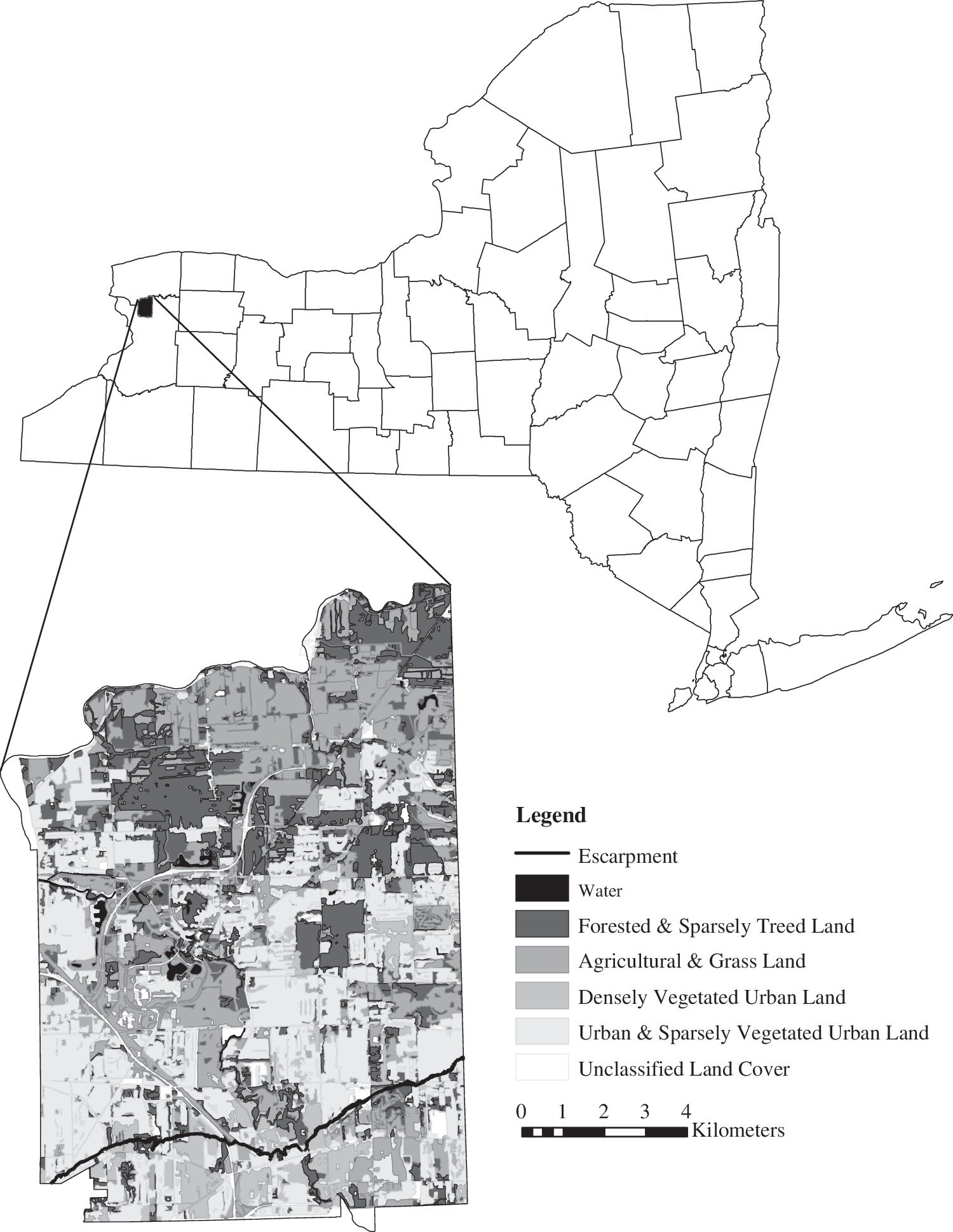
Study area map of the Town of Amherst in Erie County, NY, with land cover classes and the location of the Onondaga escarpment.

Regression trees were used to group Cx. pipiens–restuans abundance data by week of year into nine temporal categories, each consisting of two season weeks except for the first and last groups that consisted of five season weeks each (Table 1). CART analysis of Ae. vexans was more complex and resulted in 10 categories based on week of year and meteorological predictors (Fig. 2). Group 1 consists of early spring mosquito collections, group 2 consists of mosquito collections from warm and wet spring seasons, and group 3 consists of mosquito samples collected during cool and dry spring seasons. Group 3 was further broken down by season week into temporal groups 3a–3d due to the large number of observations included in this group (n = 307). Group 4 consists of mosquito samples collected from warm and dry early summer seasons. Group 5 consists of mosquito collections from warm and moist early summer seasons. Group 6 consists of mosquito samples from warm late summer seasons and group 7 consists of samples collected during cool summer seasons.

FIG. 2.

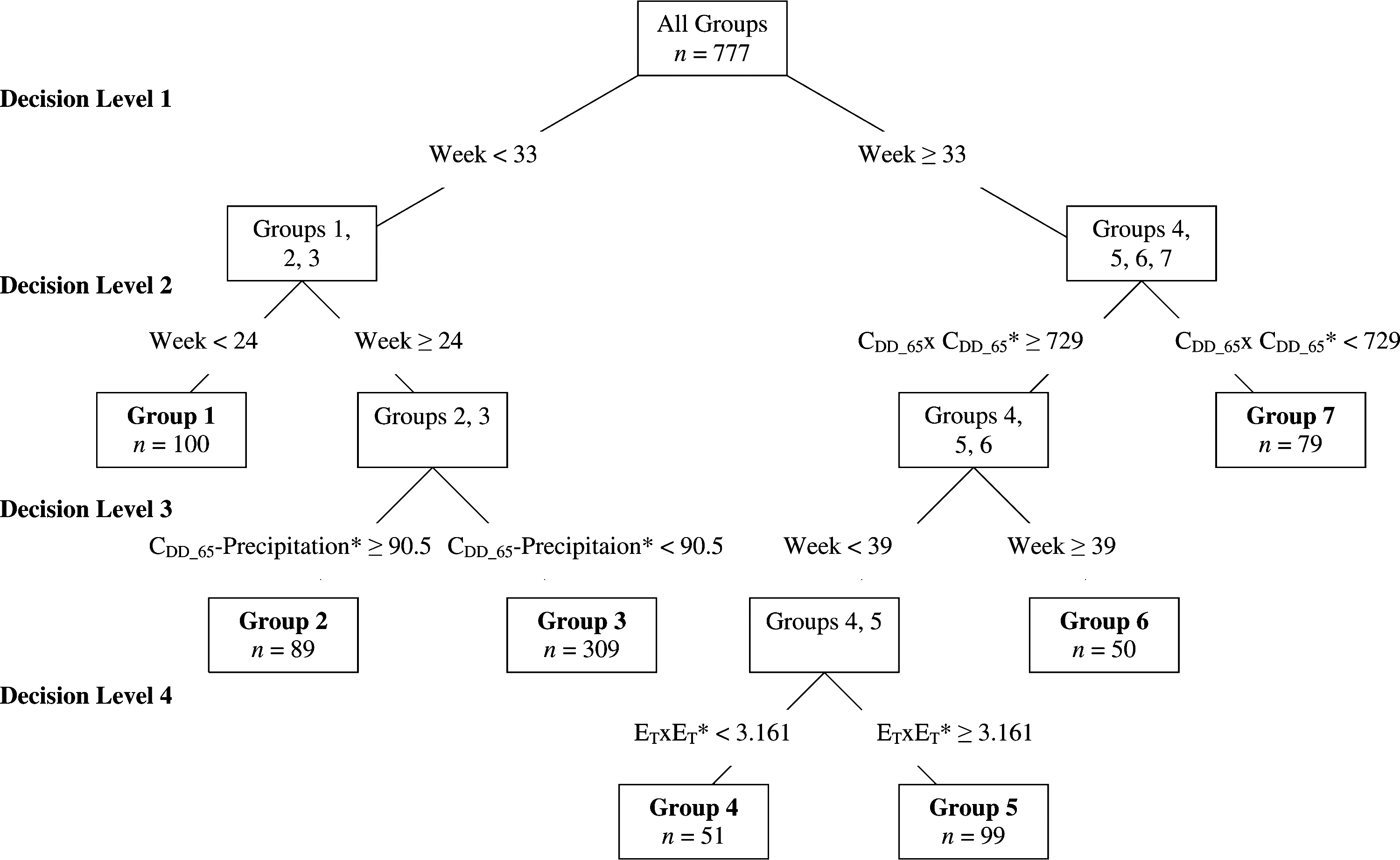
Meteorological–temporal bins of Aedes vexans as determined by regression tree analysis in Trawinski and Mackay (2009). The data are repeatedly split into groups that become more and more homogeneous at each decision level. The characteristics of each mosquito group are determined by the cumulative rules from each decision level. For example, group 2 is defined by week <33 (spring), and week ≥24 (late spring), and C_{DD_65}-precipitation ≥90.5 (warm and wet conditions) and is characterized as mosquito collections taken during warm, wet spring seasons. *The meteorological variables lagged from the mosquito abundance data: C_{DD_65}-precipitation is lagged at 2 weeks, E_T × E_T is lagged at 5 weeks, and C_{DD_65} × C_{DD_65} is lagged at 7 weeks.

Table 1.

Bins of Culex pipiens–restuans Mosquitoes Based on the Time Series and Regression Tree Analyses (Trawinski and Mackay 2009)

Group	Weeks	n
1	20–23	100
2	24–25	114
3	26–27	82
4	28–29	89
5	30–31	75
6	32–33	69
7	34–35	77
8	36–37	46
9	38–42	125

Data collection

We obtained population and housing area tables at the block level from the U.S. Census Bureau and calculated human population density, housing unit density, and median year built of housing units (Table 2). We acquired hydrography, land use, and land cover databases from the Town of Amherst Office of Information Technology. The hydrography database was comprised of hydrology and open drainage ditches that were updated from spring 1999 orthophotos with a ground pixel resolution of 0.25 ft. Land use information was coded from the 1999 Assessment Property Class Codes. Land cover information was extracted from Erie County Water Authority aerial photographs. We obtained a wetlands database from New York State Department of Environmental Conservation and floodplain areas from Federal Emergency Management Agency Flood Insurance Rate Maps. We obtained Soil Survey Geographic soils data and drainage attribute data from the Natural Resources Conservation Service. We derived elevation data from United States Geologic Survey (USGS) 7.5 min Digital Elevation Models (DEMs) and calculated slope using ArcMap Spatial Analyst (ESRI, Redlands, CA). We acquired an orthorectified Enhanced Thematic Mapper plus (ETM+) scene from National Aeronautics and Space Administration's (NASA) Landsat 7 from the repository of the Global Land Cover Facility at the University of Maryland, and calculated the Normalized Difference Vegetation Index (NDVI) (NASA Landsat Program, 1999, Landsat ETM+ scene p017r030 7x19990912ETM-EarthSat-Orthorectified, SLC-Off, USGS, Sioux Falls, 9/12/1999). NDVI was calculated as: \documentclass{aastex} \usepackage{amsbsy} \usepackage{amsfonts} \usepackage{amssymb} \usepackage{bm} \usepackage{mathrsfs} \usepackage{pifont} \usepackage{stmaryrd} \usepackage{textcomp} \usepackage{portland, xspace} \usepackage{amsmath, amsxtra} \pagestyle{empty} \DeclareMathSizes {10} {9} {7} {6} \begin{document} \begin{align*}{\rm ETM} + {\rm NDVI} = ({\rm band} \ 4 - {\rm band} \ 3) / ({\rm band} \ 4 + {\rm band} \ 3), \tag{1} \end{align*} \end{document}

Table 2.

Description of Landscape Prediction Variables and Designation as Primary or Secondary

Database	Code	Variable name	Description	Variable type
DEM	MAXSLOPE	Maximum slope	Maximum of the calculated slope	Primary
	AVGSLOPE	Average slope	Average slope as calculated from DEM	Primary
	AVGDEM	Average DEM	Average DEM value	Primary
Census	AVGHOUS	Average housing	Average housing units per square kilometer	Secondary
	AVGPOP	Average population	Average population per square kilometer	Secondary
	AVGYRBLT	Average year built	Average of median year built	Primary
	1930S	Built 1930s	Proportion of median year built in 1930s	Secondary
	1940S	Built 1940s	Proportion of median year built in 1940s	Secondary
	1950S	Built 1950s	Proportion of median year built in 1950s	Secondary
	1960S	Built 1960s	Proportion of median year built in 1960s	Secondary
	1970S	Built 1970s	Proportion of median year built in 1970s	Secondary
	1980S	Built 1980s	Proportion of median year built in 1980s	Secondary
SSURGO	W	Well drained	Soils have high hydraulic conductivity and low water holding capacity. Depth to water table more than 6 ft.	Secondary
	P	Poorly drained	Soils have a layer of low hydraulic conductivity, wet state high in the profile. Depth to water table is 3–6 ft.	Secondary
	SP	Somewhat poorly drained	Soils have intermediate water holding capacity. Depth to water table more than 6 ft.	Secondary
	MW	Moderately well drained	Soils commonly have a layer with low hydraulic conductivity, wet state in profile, etc. Depth to water table 1–3 ft.	Secondary
	SE	Somewhat excessively drained	Soils may have a saturated zone, a layer of low hydraulic conductivity, or seepage. Depth to water table less than 1 ft.	Secondary
	VP	Very poorly drained	Soils are wet to the surface most of the time. Depth to water table less than 1 ft., or is ponded.	Secondary
	ALLP	All poorly drained	Poorly and somewhat poorly combined	Secondary
	ALLW	All well drained	Well and moderately well combined	Secondary
Floodplain	A	Flood zone A	An area inundated by 100-year flooding, no BFEs determined.	Secondary
	AE	Flood zone AE	An area inundated by 100-year flooding, BFEs determined.	Secondary
	AH	Flood zone AH	An area inundated by 100-year flooding (usually an area of ponding); flood depths 1–3 ft. BFEs determined; shallow flooding.	Secondary
	X500	Flood zone X500	An area inundated by 500-year flooding; 0.2–1.0% annual risk.	Secondary
	X	Flood zone X	Areas outside the 500-year flood plain; <0.2% annual risk.	Secondary
	ALLA	All 100-year flood zones	All areas inundated by 100-year flooding, combined A flood zones, AE flood zones, and AH flood zones.	Secondary
Hydrography	HYDRO	Hydrography	Proportion of hydrography pixels in buffer	Primary
	dist_hydro	Distance to hydrography	Euclidean distance to hydrography	Primary
Land cover	SPARSE	Sparsely treed land	Sparse trees	Secondary
	FOREST	Forested Land	Forest	Secondary
	AG	Agricultural Land	Agricultural	Secondary
	GRASS	Grassland	Grassland	Secondary
	URBAN1	Urban land	Urban—general urban	Secondary
	URBAN2	Urban densely vegetated land	Urban—densely vegetated	Secondary
	URBAN3	Urban sparsely vegetated land	Urban—sparsely vegetated	Secondary
	ALLURBAN	All urban land	Combined urban areas	Primary
	TREED	Treed land	Forest and sparse trees combined	Primary
	GRASSAG	Grass and agricultural land	Grassland and agricultural areas combined	Primary
Land use	AGUSE	Agricultural land use	Agricultural	Secondary
	RES	Residential land use	Residential	Secondary
	VAC	Vacant land use	Vacant	Secondary
	COM	Commercial land use	Commercial	Secondary
	REC	Recreational land use	Recreation	Secondary
	SHE	Services land use	Services—schools, hospitals, etc.	Secondary
	MAW	Industrial land use	Industrial—manufacturing and warehouse	Secondary
	TAU	Transportation land use	Services—transportation and utilities	Secondary
	VACAGUSE	Vacant and agricultural land use	Agricultural and vacant land use categories combined	Primary
	MXURBAN	Mixed urban land use	Commercial, recreation, services, and industrial categories combined	Primary
	URBANUSE	All urban land use	Residential, commercial, recreation, services, and industrial categories combined	Primary
Wetlands	WET	Wetlands	Proportion of wetland pixels in buffer	Primary
	dist_wet	Distance to wetlands	Euclidean distance to wetlands	Primary
ETM+	NDVI	NDVI	Average calculated NDVI value from ETM+	Primary

The primary variable subset included general level 1 land use and land cover factors (Anderson 1976): urban land, agricultural land, forest, water, and wetlands and continuous variables such as NDVI and DEM. The secondary variable subset consisted of six detailed categories of variables, such as flood zones, drainage, and level 2 and level 3 land use and land cover variables from Anderson's classification system (Anderson 1976). The value for each variable was extracted for each of three buffer zones: 200, 400, and 1000 m.

DEMs, Digital Elevation Models; SSURGO, Soil Survey Geographic; BFE, base flood elevations; NDVI, Normalized Difference Vegetation Index; ETM+, Enhanced Thematic Mapper plus.

where band 4 is the near-infrared wavelength band and band 3 is the red wavelength band in ETM+ data (Lillesand and Kiefer 1994).

Geographic Information Systems (GIS) analysis

We converted all landscape variable databases to 30 × 30 m grids using ArcMap Spatial Analyst and projected the grids into Universal Transverse Mercator zone 17N projection. Each trap location was buffered to extract values of landscape variables around trap sites. We used three buffer sizes to explore the spatial scales at which each variable most contributed to the explanation of mosquito abundance. We chose buffer sizes of 200, 400, and 1000 m because previous studies indicated that landscape features were important over these distances for Ae. vexans and Cx. pipiens–restuans (Diuk-Wasser et al. 2006). We extracted values of predictor variables within each buffer as the mean value for continuous variables (i.e., DEM and NDVI) and calculated the proportion of each category in the buffer for categorical variables (i.e., land use and flood zone). The variable measuring age of housing was treated both as a continuous variable of average median year built and as a categorical variable. We also calculated Euclidean distances from each trap site to the nearest hydrographic feature or wetland pixel.

Variable selection

The goal of the statistical analysis was to determine important landscape predictors (Table 1) of mosquito abundance by group and to develop linear regression models for each group. First, variables were selected using a stepwise linear regression model with the form: \documentclass{aastex} \usepackage{amsbsy} \usepackage{amsfonts} \usepackage{amssymb} \usepackage{bm} \usepackage{mathrsfs} \usepackage{pifont} \usepackage{stmaryrd} \usepackage{textcomp} \usepackage{portland, xspace} \usepackage{amsmath, amsxtra} \pagestyle{empty} \DeclareMathSizes {10} {9} {7} {6} \begin{document} \begin{align*} \ln ({\rm Abundance} + 1) = \beta_0 + \beta_{\rm i} (X_{\rm i}) + \ldots + \beta_{\rm p} (X_{\rm p}) + e, \tag{2} \end{align*} \end{document}

where β ₀ is the intercept, β _i-β _p are the respective parameters of the independent variables, X _i-X _p are the independent variables determined by the linear regression model to produce the best model, and e is the error term. We devised a strategy to minimize multicollinearity by categorizing variables into “primary” and “secondary.” The primary variable subset included general level 1 land use and land cover factors (Anderson 1976): combined urban lands, agricultural and grass lands, forested and sparsely treed lands, water, wetlands, and continuous variables such as NDVI and DEM (Table 2). The secondary variable subset consisted of seven detailed categories of variables, such as flood zones, drainage, and level 2 and level 3 land use and land cover variables from Anderson's classification system (Anderson 1976). We selected primary and secondary variables in separate analyses conducted in stages and combined the selected variables in the last stage of model development. All primary variables were analyzed individually. The secondary variable set was analyzed by category.

We conducted variable selection with five stages of stepwise regression analysis (Fig. 3). First, we identified significant primary variables and the best buffer size for each using stepwise regression of each variable at three buffer sizes for each group (Fig. 3, result #1). Second, we combined the significant primary variables together and identified the best primary variable model (Fig. 3, result #2). Third, we analyzed each category of secondary variables with stepwise regression, one category at a time with all buffer sizes included (Fig. 3, result #3). Fourth, all the significant secondary variables were combined for analysis with stepwise regression to determine the best secondary variable model (Fig. 3, result #4). Finally, we combined the best predictors from the primary and secondary variables to develop the best overall model (Fig. 3, result #5). All stepwise linear regression analyses were conducted using SPSS version 14.0 (SPSS, Chicago, IL). All models of vector abundance and landscape predictors were tested with analysis of variance to determine their ability to explain variation in abundance. Adjusted R ² values were used to determine the strength of the relationship, and a comparison of standard error of the model estimate to the standard deviation of the abundance was made.

FIG. 3.

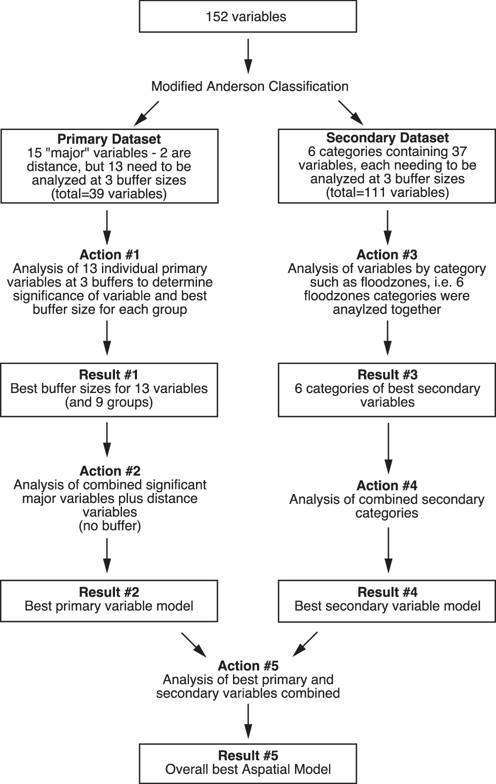
Variable selection strategy employing five stages of stepwise regression analysis.

Results

Cx. pipiens–restuans

One thousand meters was the best buffer size for the primary variables of all urban land use, mixed urban land use, average slope, and maximum slope for all groups of Cx. pipiens–restuans for which these variables were found significant. The best buffer size for the other nine primary variables depended on the time period group of Cx. pipiens–restuans examined (Trawinski and Mackay 2009) (Table 3). The best primary variable models for Cx. pipiens–restuans groups 1–9 achieved levels of explanation between 6.6% and 48.6%. Positive relationships were found between Cx. pipiens–restuans and urban land use, mixed urban land use, all urban land cover, grass and agricultural land cover, average DEM and slope, and distance to both hydrography and wetlands. Negative associations were found with tree cover, hydrography, average year built of housing, and NDVI. The effect of wetlands and vacant and agricultural land use was mixed, depending on the group of Cx. pipiens–restuans considered (Table 3).

Table 3.

Significant Major Variables by Group for Culex pipiens–restuans with Significant Buffer Size for Each Factor

Primary variables	1	2	3	4	5	6	7	8	9
URBANUSE	1000	–	–	–	–	–	1000	1000	–
	1.091						2.682	2.210
	(0.029)						(0.079)	(0.159)
MXURBAN	1000	–	–	–	–	–	–	–	–
	1.154
	(0.032)
ALLURBAN	1000	–	–	400	–	1000	1000	1000	–
	1.638			1.149		1.731	2.923	2.840
	(0.085)			(0.040)		(0.089)	(0.172)	(0.363)
VACAGUSE	1000	200	–	–	–	–	1000	1000	–
	−1.440	1.215					−2.760	−2.330
	(0.095)	(0.047)					(0.139)	(0.273)
GRASSAG	–	–	200	200	1000	–	200	–	–
			1.131	1.329	3.161		1.494
			(0.041)	(0.050)	(0.104)		(0.049)
TREED	1000	–	200	200	400	–	1000	1000	–
	−1.360		−1.422	−1.060	−1.600		−3.580	−2.610
	(0.045)		(0.066)	(0.054)	(0.066)		(0.227)	(0.236)
HYDRO	–	–	–	–	–	1000	1000	1000	–
						−14.400	−13.700	−22.800
						(0.047)	(0.046)	(0.097)
WET	200	–	–	–	200	–	1000	–	–
	1.301				−1.800		−3.570
	(0.053)				(0.092)		(0.107)
AVGDEM	400	–	–	–	–	–	200	1000	–
	0.161						0.110	0.070
	(0.057)						(0.090)	(0.090)
AVGSLOPE	–	–	–	–	–	–	1000	–	–
							1.113
							(0.114)
MAXSLOPE	–	–	–	1000	–	–	1000	–	–
				0.037			0.052
				(0.122)			(0.166)
AVGYRBLT	–	–	–	400	–	–	1000	–	200
				−0.040			−0.040		−0.030
				(0.088)			(0.091)		(0.146)
NDVI	–	–	–	–	–	–	1000	400	1000
							−10.033	−6.060	−2.390
							(0.291)	(0.203)	(0.059)
dist_hydro	–	+	–	–	–	–	+	–	+
		0.001					0.002		0.000
		(0.029)					(0.086)		(0.229)
dist_wet	–	–	+	+	–	+	+	+	+
			0.000	0.000		0.000	0.001	0.000	0.000
			(0.046)	(0.062)		(0.058)	(0.216)	(0.118)	(0.138)

Three buffer sizes were investigated for each primary landscape variable: 200, 400, and 1000 m (result #1 in Fig. 3). All variables were significant at p < 0.05. Each column of significant variables determined the input factors in the next level of stepwise regression analysis (input to action #2 in Fig. 1). Coefficients are given are in italics and adjusted R ² values are given in parentheses.

The secondary dataset was also analyzed in stages. In the first stage of analysis, each category of secondary variables was analyzed separately from the others to determine the significant variables and their most appropriate buffer size (unpublished data). In the second stage, the significant variables for each group of mosquito were combined to reveal the best overall secondary models (Table 4). The secondary variable models for Cx. pipiens–restuans revealed positive correlations with agricultural and urban land cover classes, industrial and recreational land use classes, average housing units per square kilometer, and housing built in the 1930s, 1950s, and 1980s. Negative associations were found with both forested and low tree land cover classes. The effect of vacant land use was mixed, dependent on the Cx. pipiens–restuans group being examined. The secondary variable models for Cx. pipiens–restuans groups 1–9 achieved levels of explanation between 5.0% and 51.7%, slightly higher than the primary variable models (Table 4).

Table 4.

Best Primary Variable, Secondary Variable, and Combined Stepwise Linear Regression Models as Derived from Stepwise Regression Analysis Conducted in Stages for Culex pipiens–restuans (results #2, #4, and #5 in Fig. 3)

Group	Primary model	β	R²	Secondary model	β	R²	Combined model	β	R²	SE	SD
1	VACAGUSE(1000)	− 1.334	0.095	AVGHOUS(400)	0.001	0.122	AVGHOUSE(400)	0.001	0.122	0.800	0.854
	WET(200)	1.146	0.135	AG(400)	5.360	0.171	AG(400)	5.360	0.171	0.777	–
	–	–	–	1980S(200)	1.439	0.206	1980S(200)	1.439	0.206	0.761	–
	–	–	–	VAC(1000)	− 1.078	0.243	VAC(1000)	− 1.078	0.243	0.743	–
2	VACAGUSE(200)	1.223	0.047	VAC(200)	1.251	0.050	VAC(200)	1.251	0.050	1.047	1.074
	dist_hydro	0.001	0.078	–	–	–	dist_hydro	0.001	0.081	1.030	–
3	TREED(200)	− 1.422	0.066	FOREST(200)	− 1.377	0.087	FOREST(200)	− 1.377	0.087	1.065	1.115
	–	–	–	X(200)	0.748	0.147	X(200)	0.748	0.147	1.030	–
4	MAXSLOPE(1000)	0.037	0.122	1950S(400)	0.970	0.085	MAXSLOPE(1000)	0.037	0.122	0.961	1.026
	–	–	–	1930S(400)	6.045	0.120	–	–	–	–	–
5	GRASSAG(1000)	3.161	0.104	FOREST(400)	− 1.790	0.116	FOREST(400)	− 1.790	0.116	1.060	1.128
	–	–	–	MAW(1000)	68.114	0.170	MAW(1000)	68.114	0.170	1.028	–
6	ALLURBAN(1000)	1.731	0.089	X(200)	1.043	0.148	X(200)	1.043	0.148	1.058	1.146
7	NDVI(1000)	− 9.319	0.291	X(200)	0.988	0.317	X(200)	0.988	0.317	1.035	1.252
	AVGDEM(1000)	0.072	0.334	P(400)	2.773	0.422	P(400)	2.773	0.422	0.952	–
	–	–	–	REC(1000)	5.693	0.482	REC(1000)	5.693	0.482	0.901	–
8	ALLURBAN(1000)	3.548	0.363	URBAN1(1000)	3.643	0.382	URBAN1(1000)	4.531	0.382	0.748	0.952
	HYDRO(200)	8.077	0.486	AG(200)	7.129	0.460	HYDRO(200)	8.085	0.506	0.669	–
	–	–	–	SPARSE(1000)	− 6.130	0.517	–	–	–	–	–
9	dist_hydro	0.002	0.227	1950S(1000)	1.786	0.201	dist_hydro	0.002	0.227	0.587	0.666
	dist_wet^a	0.000	0.304	–	–	–	dist_wet^a	0.000	0.304	0.557	–

Given are selected primary and secondary variables with coefficients, model-adjusted R ² values, model SEs, and SD of mosquito abundance. All variables were significant at p < 0.05.

Coefficient of dist_wet not given with enough significant digits in SPSS to give actual coefficient.

SE, standard error; SD, standard deviation.

In the final stage of analysis, the best overall model was determined by a stepwise linear analysis of the best primary and best secondary variables combined. The final combined variable stepwise linear regression models of Cx. pipiens–restuans population abundance varied according to the group examined (Table 4). Combined variable models for Cx. pipiens–restuans groups 1–9 achieved levels of explanation between 8.1% and 50.6% with the best overall models sometimes containing all primary variables (groups 4 and 9), sometimes all secondary variables (groups 1, 3, 5, 6, and 7), and sometimes a combination of primary and secondary variables (groups 2 and 8). Cx. pipiens–restuans group 4 was best modeled with only the primary variable of maximum slope. In contrast, Cx. pipiens–restuans group 8 was best modeled with both the secondary variable of general urban land and the primary variable of hydrography. All variables retained for analysis were significant at p < 0.05.

Ae. vexans

The best buffer size was 1000 m for all urban land use, mixed urban land use, vacant and agricultural land use, wetlands, average slope, and average year built (Table 5). The best buffer size was 200 m for combined urban land cover, grass and agricultural land, and hydrography. The 400-m buffer size was best only for average elevation. Best buffer size varied for the tree cover variable and maximum slope. NDVI was not significant for any of the tested buffer sizes. Interestingly, most of the significant 200-m buffers were found in groups representing spring collections, whereas most of the significant 1000-m buffers were found in groups collected during the summer.

Table 5.

Significant Major Variables by Group for Aedes vexans with Significant Buffer Size for Each Factor

Primary variables	1	2	3a	3b	3c	3d	4	5	6	7
URBANUSE							1000			1000
	–	–	–	–	–	–	−2.538	–	–	−1.929
							(0.096)			(0.057)
MXURBAN							1000
	–	–	–	–	–	–	−3.887	–	–	–
							(0.184)
ALLURBAN	200	200
	−0.405	1.751	–	–	–	–	–	–	–	–
	(0.043)	(0.062)
VACAGUSE					1000
	–	–	–	–	−1.312	–	–	–	–	–
					(0.041)
GRASSAG	200		200
	0.446	–	2.978	–	–	–	–	–	–	–
	(0.038)		(0.093)
TREED			200	–	1000
	–	–	−1.952		−1.528	–	–	–	–	–
			(0.060)		(0.040)
HYDRO							200
	–	–	–	–	–	–	11.867	–	–	–
							(0.131)
WET	–	–	–	1000	–	–	–	–	1000	1000
				3.281					4.609	3.488
				(0.066)					(0.071)	(0.198)
AVGDEM					400
	–	–	–	–	0.081	–	–	–	–	–
					(0.035)
AVGSLOPE				1000						1000
	–	–	–	−2.438	–	–	–	–	–	–0.772
				(0.121)						(0.110)
MAXSLOPE	1000
	0.021	–	–	–	–	–	–	–	–	–
	(0.040)
AVGYRBLT						1000
	–	–	–	–	–	0.050	–	–	–	–
						(0.075)
NDVI	–	–	–	–	–	–	–	–	–	–
dist_hydro	–	–	–	–	–	–	–	–	–	–
dist_wet	–	–	–	–	–	–	–	–	–	–

Three buffer sizes were investigated for each primary landscape variable: 200, 400, and 1000 m (result #1 in Fig. 3). All variables were significant at p < 0.05. Each column of significant variables determined the input factors in the next level of stepwise regression analysis (input to action #2 in Fig. 3). Coefficients are given are in italics and adjusted R ² values are given in parentheses.

Stepwise linear regression analysis of primary variables revealed negative associations with all urban land, mixed urban land use, vacant and agricultural land use, and average slope for all groups of Ae. vexans (Table 6). Positive correlations were found for wetlands, hydrography, average year built, and grass and agricultural land with Ae. vexans abundance across all groups. These variables were significant (p < 0.05), but individually explained only 4% to 25% of the variance in Ae. vexans abundance in each meteorological group. Model R ² values varied between 0.041 and 0.246 (Table 6).

Table 6.

Best Primary Variable, Secondary Variable, and Combined Stepwise Linear Regression Models as Derived from Stepwise Regression Analysis Conducted in Stages for Aedes vexans (results #2, #4, and #5 in Fig. 3)

Group	Primary model	β	R²	Secondary model	β	R²	Combined model	β	R²	SE	SD
1	ALLURBAN(200)	− 0.405	0.043	URBAN1(200)	− 0.483	0.064	URBAN1(200)	− 0.483	0.064	0.379	0.392
2	ALLURBAN(200)	− 1.751	0.062	URBAN1(200)	− 1.517	0.073	URBAN1(200)	− 1.517	0.073	1.227	1.274
	–	–	–	1930s(200)	25.660	0.108	1930S(200)	25.660	0.108	1.203	–
	–	–	–	AGUSE(400)	12.005	0.145	AGUSE(400)	12.005	0.145	1.178	–
3a	GRASSAG(200)	2.978	0.093	FOREST(200)	− 2.597	0.124	FOREST(200)	− 2.597	0.124	1.495	1.600
3b	AVGSLOPE(1000)	− 2.438	0.121	X500(1000)	2.411	0.171	X500(1000)	2.411	0.171	1.384	1.521
3c	VACAGUSE(1000)	− 1.312	0.041	AVGHOUS(1000)	0.001	0.072	AVGHOUS(1000)	0.001	0.072	1.149	1.193
	–	–	–	SPARSE(1000)	− 6.202	0.103	SPARSE(1000)	− 6.202	0.103	1.130	–
	–	–	–	COM(1000)	− 5.226	0.135	COM(1000)	− 5.226	0.135	1.109	–
3d	AVGYRBLT(1000)	0.500	0.075	1980S(200)	0.899	0.055	AVGYRBLT(1000)	0.500	0.075	1.426	1.483
4	MXURBAN(1000)	− 3.223	0.184	RES(1000)	− 3.918	0.169	MXURBAN(1000)	− 3.223	0.184	1.252	1.385
	HYDRO(200)	8.827	0.246	–	–	–	HYDRO(200)	8.827	0.246	1.203	–
5	–	–	–	ALLA(400)	− 1.391	0.043	ALLA(400)	− 1.391	0.043	1.445	1.633
6	WET(1000)	4.609	0.071	AE(200)	− 1.895	0.134	AE(200)	− 1.895	0.134	1.630	1.751
	–	–	–	AG(200)	23.723	0.216	AG(200)	23.723	0.216	1.550	–
7	WET(1000)	3.904	0.198	1980S(200)	0.806	0.062	WET(1000)	3.904	0.198	1.022	1.142

Given are selected primary and secondary variables with coefficients, model-adjusted R ² values, model SEs, and SD of mosquito abundance. All variables were significant at p < 0.05.

The best secondary variable models revealed negative correlations between Ae. vexans abundance and general urban, forested, and low tree land cover classes, commercial and residential land uses, and areas inundated by 100-year flooding (Table 6). Positive associations were found with housing built in the 1930s and 1980s, average housing units per square kilometer, agricultural land cover and land use classes, and areas inundated by 500-year flooding. These variables were significant (p < 0.05), but individually explained only 4.3% to 21.6% of the variance in Ae. vexans abundance in each meteorological group (Table 6).

The R ² values for the best combined Ae. vexans models range between 0.043 and 0.246 (Table 6). General urban land cover is a negative covariate for Ae. vexans group 2, with agricultural land use and proportion of housing built in the 1930s as positive covariates. Group 7 represents the highest population abundance of all Ae. vexans groups. The only significant landscape factor retained for this group was the proportion of wetlands in a 1000-m buffer. All variables retained for analysis were significant at p < 0.05.

Discussion

We determined the scale at which various landscape elements affected mosquito abundance by testing each landscape variable at three buffer sizes. Most studies use a 1000-m buffer based on the average flight range of mosquitoes (Beck et al. 1997, Moncayo et al. 2000, Diuk-Wasser et al. 2006). A notable exception is the study by Diuk-Wasser et al. (2006), which investigated the scale of influence for 10 buffer sizes between 100 and 1000 m. It was expected that landscape proportions in the smaller buffer distances would be highly significant for Cx. pipiens–restuans distribution because of the smaller flight range of this species. However, the 1000-m buffer was significant more often than the other buffer sizes for this species (Table 3). Twenty-six (22.2%) of the primary variables tested were significant for the 1000-m buffer size, 5 (4.3%) were significant for the 400-m size, 10 (8.5%) were significant for the 200-m size, and 76 (65.0%) were not significant at any buffer size. For Ae. vexans, 12 (9.2%) primary variables were significant for the 1000-m buffer, 1 (0.8%) was significant for the 400-m buffer, 6 (4.6%) were significant for the 200-m buffer, and 121 (93.1%) primary variables were not shown to influence Ae. vexans abundance for any buffer size (Table 5). Overall, our results do not completely agree with Diuk-Wasser et al. (2006), who showed that buffer sizes smaller than 1000 m were most significant for all variables except the water variable. However, important differences exist between the two studies, the main one being their use of logistic regression analysis to determine high and low abundance over a larger area (two counties) of more varied landscape. Our study area is primarily suburban, and larger buffer sizes may reflect correlation over longer distances because of the spatial extent of the built-up landscape and the relatively low variance of the environmental variables for this type of landscape. In the future, tests for the influence of landscape features on Cx. pipiens–restuans abundance should be conducted in varying landscapes to assess differences in urban, suburban, and rural environments.

Primary and secondary landscape covariates support the known bionomics of both Ae. vexans and Cx. pipiens–restuans mosquitoes with few exceptions. Urban areas, grass and agricultural land, average elevation, average and maximum slope, and distance to both wetlands and hydrography were positive landscape covariates of Cx. pipiens–restuans abundance in all groups, in accordance with the known ecological habitats preferred by Cx. pipiens–restuans. Urban land use was an important predictor of the abundance of this species, reflecting its affinity for stagnant water and urban areas where artificial containers of water are numerous. The effects of urban areas had the strongest explanatory power for late-season Cx. pipiens–restuans abundance (Table 1). Other studies have reported a similar correlation between urban population density and Cx. pipiens–estuans population abundance (Andreadis et al. 2004, Diuk-Wasser et al. 2006). Grass and agricultural land had a positive effect on Cx. pipiens–restuans abundance as well, possibly indicating an increased abundance of this species in suburban environments. Cx. pipiens–restuans is most often associated with urban environments, but recent studies have indicated suburban areas to be important habitats of this species as well (Diuk-Wasser et al. 2006). Positive influences of elevation and slope may be accounted for by the urban density generally increasing southward along with elevation increases toward the Onondaga Escarpment in Amherst. Significant relationships between distance-to-wetlands and distance-to-hydrographic feature with Cx. pipiens–restuans abundance may be explained by general increases in urban density in the western and southwestern portions of Amherst. Landscape features that had a primarily negative effect on Cx. pipiens–restuans populations were wetlands, hydrography, tree cover, vacant and agricultural land, and NDVI. NDVI was the best single primary covariate for group 7 with explanatory power of 29.1%. Brownstein et al. (2002) identified an increase in human WNv risk with increased NDVI up to a threshold value of 0.22 for the original outbreak in New York City, but that relationship was based on the ecology of mosquitoes in a metropolitan area. Lower values of NDVI may indicate urban build up, and the inverse relationship with Cx. pipiens–restuans abundance was expected in a suburban town such as Amherst. Older housing was positively associated with Cx. pipiens–restuans. Generally, areas of older housing are the more densely populated areas of Amherst and these houses may have accumulated more artificial water containers. Negative correlations were found between Cx. pipiens–restuans abundance and tree cover for six mosquito abundance groups, supporting research by Diuk-Wasser et al. (2006) which found forests having a negative effect on Cx. pipiens–restuans abundance. Levels of explanation achieved through inclusion of environmental covariates varied between 8.1% and 50.6% for the best models developed for Cx. pipiens–restuans groups based on time. However, 15% of the overall variation in Cx. pipiens–restuans population abundance has already been accounted for by the temporal analysis (Trawinski and Mackay 2008) and when considered incrementally total levels of explanation vary between 23% and 65%.

Positive covariates for Ae. vexans indicated the wet conditions preferred by this species: wetlands, hydrography, elevation, grassland, and agricultural land. Proportion of wetlands is the best covariate when Ae. vexans abundance is at a maximum, supporting previous research indicating wetlands and frequently flooded areas to be highly correlated with Ae. vexans (Hayes et al. 1985, Moncayo et al. 2000). Positive correlations of Ae. vexans abundance with water and grasslands/agriculture are also supported by previous research (Diuk-Wasser et al. 2006). Negative covariates for Ae. vexans were urban areas, tree covered land, average slope, and vacant and agricultural land. The inverse relationship between urban areas and Ae. vexans population abundance most likely reflects trends in housing development because areas less prone to flooding are normally developed before wet areas with flooding problems. No significant relationships were found with NDVI, distance to wetlands, or distance to hydrography. Final landscape models indicate that physical covariates explained between 6.4% and 24.6% of Ae. vexans population abundance. It was expected that landscape factors would have a small influence on this species because meteorological conditions have already explained 55% of the overall variance in this species (Trawinski and Mackay 2008). Overall, hierarchical analysis including predictive meteorological and landscape covariates explained between 61% and 80% of the variation in Ae. vexans abundance.

The current research was unique in addressing the level of detail needed to predict locations at a high risk for WNv through the designation of primary and secondary variables. The analysis of the secondary set of variables supported the results from the primary variables set for Ae. vexans. Positive effects of secondary agricultural land cover and land use variables reinforced the general positive trend for the primary variable grass and agricultural land. Specific urban land use categories negatively correlated with Ae. vexans were commercial, residential, and mixed urban. A positive effect was found for average housing unit density and abundance of Ae. vexans in the cool, dry late spring group (group 3c), probably reflecting increases in urban density occurring in the northern portion of Amherst and general encroachment of humans in Ae. vexans habitats. Forested land and sparsely forested land were negative effects, which reinforced the results seen by the primary variable tree cover. Certain types of forests may affect Ae. vexans abundance differently depending on the wetness of soil preferred by different stands of trees. Another possible explanation for this relationship may be that adult Ae. vexans are traveling away from seasonally wet breeding areas toward potential blood meals in more urbanized areas.

Analysis of secondary variables reinforced the relationships found between Cx. pipiens–restuans abundance and the primary variable set and revealed the effects of more specific landscape elements. Industrial and recreational areas were positively associated with Cx. pipiens–restuans abundance during weeks 30–31 and weeks 34–35 (Table 1). Average density of housing was the most significant effect early in the season, explaining over 12% of the variation in group 1 (p < 0.001). Housing from the 1980s also had a positive effect during this time period, possibly indicating an increase in Cx. pipiens–restuans abundance as housing developments have become established in previously rural sections of Amherst. Agricultural land and poorly drained areas were shown to have significant positive effects on Cx. pipiens–restuans abundance and a definitive explanation for these relationships remains elusive. One possibility is that these areas are perennially flooded. Hayes et al. (1985) indicated that permanently flooded areas have the highest potential for Culex species mosquitoes. Another possibility is that these areas are adjacent to urban areas. Also the negative effects of forested and sparsely treed land reinforced the general trend illustrated by the primary variable tree cover, though the scale of influence is not constant for this landscape feature.

The best primary and secondary Ae. vexans and Cx. pipiens–restuans models achieved similar levels of explanation. Overall, spatially distributed predictive variables were more important for explanation of Cx. pipiens–restuans population abundance than for Ae. vexans population abundance. The best primary variable models explained between 4.1% and 24.6% of the Ae. vexans abundance, whereas the best secondary variable models explained between 4.3% and 21.6% of the abundance. For most groups the best secondary variable models had slightly more predictive power with a mean R ² value of 11.84 for the best secondary variable models and a mean R ² value of 9.50 for the best primary variable models. The best primary variable regression equations developed for Cx. pipiens–restuans explained between 6.6% and 48.6% of the population abundance, whereas the best secondary variable regression equations explained between 5.0% and 51.7% of the variation. The mean R ² value was 0.191 for the best primary variable models and 0.231 for the best secondary variable models.

Several shortcomings to the current research can be identified. Though Cx. pipiens and Cx. restuans are often grouped due to difficulties in distinguishing the two species, they are distinct species with Cx. restuans abundance at a maximum in the early summer and crossover occurring in mid-summer, after which point Cx. pipiens is the dominant species. This should not significantly affect our results because the groups of Cx. pipiens–restuans are based on time. In effect, the early groups represent Cx. restuans with the later groups representing Cx. pipiens. Another possible shortcoming of the current study is the spatial dependence inherent in ecological data that may change the significance level of an effect. However, this study is a necessary step toward combining interpolation methods and landscape methods of prediction and future studies in which these techniques are combined are planned by the authors.

Conclusions

We identified landscape elements important for distribution and abundance of two WNv vector mosquitoes and developed models for groups of mosquitoes based on time and meteorological conditions. Landscape elements were shown to have a significant effect on Cx. pipiens–restuans population abundance. The structure of the landscape had a lesser impact on the abundance of Ae. vexans in the study area. The different effects of ecosystem structure between the two species studied may be attributed to the flight ranges of the mosquitoes. The flight range of Cx. pipiens–restuans differs markedly from the flight range of Ae. vexans. Thus, landscape structure at the neighborhood scale investigated here has a lesser effect on the population dynamics of Ae. vexans but is critical for prediction of Cx. pipiens–restuans. Importantly, this study demonstrated that late-season abundance of Cx. pipiens–restuans predictions are the most accurate. Epidemics of WNv in humans tend to occur in the late summer and predictions of the most important vector in the northeastern United States during the high risk time of year will enable prevention and control efforts to minimize human disease.

Our method of variable selection conducted in stages was designed to extract information about the level of detail needed in variables to make predictions of mosquito abundance as a proxy for disease risk. Multicollinearity was not problematic with variable selection conducted in stages. Though some models were decidedly better with the secondary variables included, in some cases the primary variable models outperformed other models that included more detailed landscape variables. Many municipalities do not have personnel employed to obtain and create data for use in geographic information systems and creation of such data may be cost prohibitive. These municipalities still have mosquito problems and knowledge of major landscape features associated with specific vector species will assist in mosquito control. Reasonable predictions could possibly be made for late-season Cx. pipiens–restuans populations with knowledge of urban areas and hydrographic features, which are readily available data for most communities.

Footnotes

Acknowledgments

The authors would like to thank Paula Thompson and Dave Muck from the Town of Amherst Highway Department, Mosquito Control Program, and Peter Tripi, Glenn Robert, and John Eiss of the Erie County Health Department, Vector Control Program, for providing the mosquito trapping data. The authors also thank Dr. Ling Bian and Dr. Peter Rogerson and the anonymous reviewers for helpful comments.

Disclosure Statement

No competing financial interests exist.

References

Anderson

. A Land Use and Land Cover Classification System for Use with Remote Sensor Data. United States Government Print Office: New York, 1976.

Andreadis

, Anderson

, Vossbrinck

, Main

. Epidemiology of West Nile virus in Connecticut: a five-year analysis of mosquito data 1999–2003. Vector Borne Zoonot Dis, 2004; 4:360–378.

Barnes

, Cibula

. Some implications of remote sensing technology in insect control programs including mosquitoes. Mosq News, 1979; 39:271–282.

Beck

, Rodriguez

, Dister

. Assessment of a remote sensing-based model for predicting malaria transmission risk in villages of Chiapas, Mexico. Am J Trop Med Hyg, 1997; 56:99–106.

Beck

, Rodriguez

, Dister

, Rodriguez

et al. Remote sensing as a landscape epidemiologic tool to identify villages at high risk for malaria transmission. Am J Trop Med Hyg, 1994; 5:271–280.

Brown

, Childs

, Diuk-Wasser

, Fish

. Ecological factors associated with West Nile virus transmission, northeastern United States. Emerg Infect Dis, 2008; 14:1539–1545.

Brownstein

, Rosen

, Purdy

, Miller

et al. Spatial analysis of West Nile virus: Rapid risk assessment of an introduced vector-borne zoonosis. Vector Borne Zoonot Dis, 2002; 2:157–164.

De'ath

, Fabricius

. Classification and regression trees: a powerful yet simple technique for ecological data analysis. Ecology, 2000; 81:3178–3192.

DeGaetano

. Meteorological effects on adult mosquito (Culex) populations in metropolitan New Jersey. Int J Biometeorol, 2005; 49:345–353.

10.

Dister

, Fish

, Bros

, Frank

et al. Landscape characterization of peridomestic risk for Lyme disease using satellite imagery. Am J Trop Med Hyg, 1997; 57:687–692.

11.

Diuk-Wasser

, Brown

, Andreadis

, Fish

. Modeling the spatial distribution of mosquito vectors for West Nile virus in Connecticut, USA. Vector Borne Zoonot Dis, 2006; 6:283–295.

12.

Glass

, Schwartz

, Morgan

III , Johnson

et al. Environmental risk factors for Lyme disease identified with geographic information systems. Am J Public Health, 1995; 85:944–948.

13.

Hayes

, Maxwell

, Mitchell

, Woodzick

. Detection, identification, and classification of mosquito larval habitats using remote sensing scanners in earth-orbiting satellites. Bull World Health Organ, 1985; 63:361–374.

14.

Hugh-Jones

, Barre

, Nelson

, Wehnes

et al. Landsat-TM identification of Amblyomma variegatum (Acari: Ixodidae) habitats in Guadeloupe. Remote Sens Environ, 1992; 40:43–55.

15.

Kilpatrick

, Kramer

, Campbell

, Alleyne

et al. West Nile virus risk assessment and the bridge vector paradigm. Emerg Infect Dis, 2005; 11:425–429.

16.

Lillesand

, Kiefer

. Remote Sensing and Image Interpretation. New York: John Wiley & Sons, Inc., 1994.

17.

Maupin

, Fish

, Zultowsky

, Campos

et al. Landscape ecology of Lyme disease in a residential area of Westchester County, New York. Am J Epidemiol, 1991; 133:1105–1113.

18.

Moncayo

, Edman

, Finn

. Application of geographic information technology in determining risk of eastern equine encephalomyelitis virus transmission. J Am Mosq Control Assoc, 2000; 16:28–35.

19.

Pope

, Rejmankova

, Savage

, Arredondo-Jimenez

et al. Remote sensing of tropical wetlands for malaria control in Chiapas, Mexico. Ecol Appl, 1994; 4:81–90.

20.

Pope

, Sheffner

, Linthicum

, Bailey

et al. Identification of central Kenyan Rift Valley fever virus vector habitats with Landsat TM and evaluation of their flooding status with airborne imaging radar. Remote Sens Environ, 1992; 40:185–196.

21.

Pratt

, Moore

. Mosquitoes of Public Health Importance and Their Control. Atlanta, GA: Centers for Disease Control and Prevention, United States Department of Health and Human Services, 1993.

22.

Trawinski

, Mackay

. Meteorologically conditioned time-series predictions of West Nile virus vector mosquitoes. Vector Borne Zoonot Dis, 2008; 8:505–522.

23.

Trawinski

, Mackay

. Spatial autocorrelation of West Nile virus vector mosquito abundance in a seasonally wet suburban environment. J Geogr Syst, 2009; 11:67–87.

24.

Turell

, Dohm

, Sardelis

, O'guinn

et al. An update on the potential of North American mosquitoes (Diptera: Culicidae) to transmit West Nile virus. J Med Entomol, 2005; 42:57–62.

25.

Turell

, O'Guinn

, Oliver

. Potential for New York mosquitoes to transmit West Nile virus. Am J Trop Med Hyg, 2000; 62:413–414.

26.

Wagner

, Hill-Rowley

, Narlock

, Newson

. Remote sensing: a rapid and accurate method of data acquisition for a newly formed mosquito control district. Mosq News, 1979; 30:283–287.

27.

White

, Andrew

, Mans

, Ohajuruka

et al. West Nile virus in mosquitoes of northern Ohio, 2003. Am J Trop Med Hyg, 2006; 75:346–349.

28.

Wood

, Beck

, Washino

, Hibbard

et al. Estimating high mosquito-producing rice fields using spectral and spatial data. Int J Remote Sens, 1992; 13:2813–2826.

29.

Wood

, Beck

, Washino

, Palchick

et al. Spectral and spatial characterization of rice field mosquito habitat. Int J Remote Sens, 1991; 12:621–626.