A Proposed Solution to the Problem With Using Completely Random Data to Assess the Number of Factors With Parallel Analysis

Abstract

A number of psychometricians have argued for the use of parallel analysis to determine the number of factors. However, parallel analysis must be viewed at best as a heuristic approach rather than a mathematically rigorous one. The authors suggest a revision to parallel analysis that could improve its accuracy. A Monte Carlo study is conducted to compare revised and traditional parallel analysis approaches. Five dimensions are manipulated in the study: number of observations, number of factors, number of measured variables, size of the factor loadings, and degree of correlation between factors. Based on the results, the revised parallel analysis method, using principal axis factoring and the 95th percentile eigenvalue rule, offers promise.

Keywords

factor analysis number of factors parallel analysis

Researchers frequently use exploratory factor analysis to establish factors that could explain in a parsimonious and meaningful way the covariation among a set of measures. Empirical criteria are frequently applied to suggest the number of factors that should be extracted. Horn (1965) and others (e.g., Fabrigar, Wegener, MacCallum, & Strahan, 1999; Preacher & MacCallum, 2003) have argued that the popular eigenvalue-greater-than-one criterion (Guttman, 1954; Kaiser, 1960) does not perform well, and parallel analysis, perhaps in conjunction with other criteria such as the scree test (Cattell, 1978), should be used to determine the number of factors. Since Horn (1965) first presented parallel analysis, a number of researchers have suggested how parallel analysis might be modified to improve its accuracy (e.g., Buja & Eyuboglu, 1992; Glorfeld, 1995; Humphreys & Montanelli, 1975). Nevertheless, no parallel analysis method appears uniformly better than others across a wide range of population conditions (e.g., Crawford et al., 2010).

All parallel analysis methods include the generation of comparison data sets containing completely random data to assess the number of factors. As suggested by previous researchers (Harshman & Reddon, 1983; Turner 1998), the general use of comparison data sets with completely random data is flawed. In this article, we offer an approach that should at least partially correct this problem, particularly with well-defined factor structures, and evaluate this proposed approach using a Monte Carlo study.

Brief Literature Review of Parallel Analysis

There are multiple approaches for conducting a parallel analysis (Glorfeld, 1995; Horn, 1965; Zwick & Velicer, 1986). One common method involves performing a principal component analysis on an observed correlation matrix. Next, multiple correlation matrices (e.g., 100 matrices) are generated assuming uncorrelated multivariate normally distributed population data with the same number of variables and sample size as the observed data. Principal component analysis is conducted on each of these random correlation matrices. The mean eigenvalues for the sequential components are computed. The assessed number of dimensions is equal to the number of eigenvalues for the observed data that exceed the respective means of eigenvalues for the random data. Figure 1 is an example of results from a parallel analysis based on principal component analysis with mean eigenvalues; the results indicate three dimensions.

Figure 1.

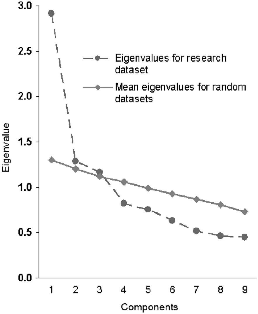
Illustration of traditional parallel analysis based on principal component analysis and the mean eigenvalue criterion

Some methodologists have advocated using common factor methods for conducting parallel analysis rather than principal component analysis (e.g., Ford, MacCallum, & Tait, 1986; Humphreys & Montanelli, 1975). They argue that common factor methods should be used to assess the factor structure of educational and psychological scales in that the model underlying these methods allows for measurement error in scales, whereas the model for principal component analysis does not (e.g., Fabrigar et al., 1999; Snook & Gorsuch, 1989; Widaman, 1993). To be consistent, researchers should use common factor analytic methods in conducting their parallel analyses if they plan to apply these methods to determine the underlying structure of their scales. More technically speaking, Mulaik (2010, p. 195) states in the revision of his classic book on factor analysis that the major failing of the parallel analysis method is that it is “based on eigenvalues of the wrong matrix.” He then points out that the rationale underlying Thurstone’s minimum rank concept is based not on the correlation matrix but the reduced correlation matrix with communalities along the diagonal. Nevertheless, the majority of research on the application of parallel analysis has used principal component analysis (Steger, 2006; Velicer, Eaton, & Fava, 2000).

Zwick and Velicer (1986) found parallel analysis showed a slight tendency toward extracting “minor components,” especially with lower factor loadings and smaller sample sizes. This finding has supported the belief that parallel analysis tends to overextract factors and has encouraged the use of a more stringent criterion in the form of the 95th or 99th percentile of the distribution of eigenvalues from the random data, which reduces the number of factors extracted (e.g., Buja & Eyuboglu, 1992; Glorfeld, 1995; Turner, 1998). Potentially, the application of these more stringent criteria could be used with parallel analyses based on common factor analytic or principal component analytic methods.

Recently, Crawford et al. (2010) compared the performance of parallel analysis using principal component analysis and parallel analysis using principal axis factoring to identify the number of underlying factors. Additionally, the accuracies of the mean eigenvalue and the 95th percentile eigenvalue criteria were examined. The 95th percentile criterion was preferable for assessing the first eigenvalue using either extraction method. In assessing subsequent eigenvalues, parallel analysis using principal component analysis tended to perform as well as or better than parallel analysis with principal axis factoring for models with one factor or multiple, minimally correlated factors, with neither eigenvalue criterion showing uniform superiority. If the factors were more than minimally correlated, parallel analysis based on principal axis factoring using the mean eigenvalue criterion generally performed best. Overall, the results were complex and did not allow for a single recommendation about what particular parallel analysis method or methods should be used in practice.

A Conceptual Flaw With Traditional Parallel Analysis Methods

Under the hypothesis that the data have k underlying factors, the rationale for applying a traditional parallel analysis using the 95th percentile rule is that the empirical distribution of the kth + 1 eigenvalue from factor or component analyses of comparison data sets constitutes an appropriate reference distribution. The use of the 95th percentile rule embodies a decision rule akin to a hypothesis testing framework with α = .05. Theoretically, this rationale may be legitimate for evaluating the hypothesis that there are no common factors (i.e., k = 0) in that the empirical distribution of the 1st eigenvalue (i.e., k + 1 = 1) from the analysis of the comparison data sets represents the sampling distribution under the null hypothesis that there are no common factors. However, this rationale for traditional parallel analysis methods is problematic for evaluating the remaining eigenvalues, as the empirical distribution of eigenvalues beyond the first one is conditioned on the presence of zero factors rather than k factors (Harshman & Reddon, 1983; Turner, 1998). From this perspective, parallel analysis must be viewed as a heuristic approach rather than a mathematically rigorous method resting on a solid conceptual base.

Turner (1998) demonstrated this problem with parallel analysis by generating data sets containing 10 variables with a sample size of either 100 or 1,000. Underlying the 10 variables was either no factors or a single factor that accounted for 30% or 50% of the total variance. The 2nd through 10th eigenvalues for data sets with one underlying factor were, on average, smaller than the eigenvalues for data sets with no underlying factors. In addition, the difference was greater when the sample size was small and the percentage of variance accounted for by the factor was large. Extrapolating from these results, if the number of factors is k, then the eigenvalues beyond the kth factor for random data in parallel analysis are positively biased and, therefore, could result in underfactoring.

The Revised Parallel Analysis Method

Recognizing this flaw in parallel analysis, Turner (1998) suggested that the appropriate reference distribution for evaluating the need for the kth + 1 factor is one in which the previous k factors have been modeled or incorporated. However, no specific procedure for modeling factors has been advanced or investigated based on our review of the literature. We next propose a method and then investigate the validity of the newly proposed approach.

The revised parallel analysis procedure is designed to allow for a more accurate assessment of the eigenvalue for the kth + 1 factor by taking into account the existence of k prior factors. Ideally, the multiple data sets for a parallel analysis should be generated based on the loadings of the k factors for the population from which the data were sampled. Because the population factor loadings are unknown, the sample factor loadings are substituted for the population values in conducting a revised parallel analysis. Results from this analysis should be more accurate to the extent that sample results are more stable and the factor structure is well defined. In other words, revised parallel analysis should yield more satisfactory results with large sample sizes and factor structures with high factor loadings, large number of measures per factor, and low correlation between factors.

We now describe revised parallel analysis in greater detail. As with traditional parallel analysis, a factor analysis is initially conducted on the observed data set, with N_V variables and N_O subjects. The statistics from the factor analysis required by revised parallel analysis include the eigenvalues and standardized loadings for the unrotated factors. Next, as described below, a 5-step approach is used to generate multiple comparison data sets based on a model with k underlying factors. The comparison data sets are factor analyzed and their results, in conjunction with the factor analytic results from the observed data set, are evaluated. This 5-step approach is applied initially using comparison data sets with 0 underlying factors (i.e., k = 0), then with 1 underlying factor (i.e., k = 1), and so on (i.e., k = 2, 3, . . .) until the decision about the inferred number of factors is made. We describe the 5-step approach as follows.

Step 1

Generate 100 comparison data sets (or more, if one prefers greater precision) with N_V variables and N_O subjects. The data are generated assuming k factors based on the following equation:

X = F Λ^{'} + E,

where X is a N_O × N_V matrix containing the scores on the variables, F is a N_O × N_k matrix containing generated scores on the factors, Λ is the N_V × N_k matrix containing the standardized loadings for k factors from the analysis based on the observed data set, and E is a N_O × N_V matrix containing generated residual scores for the variables. The factor scores are assumed to be independently and normally distributed with a mean of zero and a variance of 1. The error scores for a variable are assumed to be independently and normally distributed with a mean of zero and a variance equal to 1 minus the sum of the k squared loadings for the variable of interest. If k = 0, then X = E.

Step 2

Conduct a factor analysis on each of the 100 comparative data sets generated in Step 1. Determine the eigenvalue for the kth + 1 factor for each of these data sets.

Step 3

Compute a summary statistic (e.g., mean or 95th percentile) of the 100 eigenvalues for the kth + 1 factor determined in Step 2.

Step 4

If the eigenvalue for the kth + 1 factor for the observed data set is less than the summary statistic (e.g., mean or 95th percentile) of the eigenvalues for the kth + 1 factor for the comparative data sets, then the parallel analysis is completed, and the number of factors underlying the observed data is inferred to be k. Otherwise, the number of factors underlying the sample data is inferred to be at least k + 1 factors unless contraindicated by the results of Step 5.

Step 5

This step is required if the parallel analysis is based on principal axis factoring or is optional if it is based on principal component analyses. If the eigenvalue for the kth + 1 factor for the observed data set is less than or equal to zero with principal axis factoring or less than one with principal components, then the parallel analysis is completed, and the number of factors underlying the observed data is inferred to be k. If the parallel analysis proceeds based on the results of Steps 4 and 5, then k is incremented by 1, and Steps 1 through 5 are repeated.

The last step was required to take into account nonpositive eigenvalues based on principal axis factoring with observed data sets. A zero or negative eigenvalue indicates that a factor has zero or negative variance. In practice, no well-trained researcher extracts factors with zero or negative variance. Accordingly, Step 5 reflects good practice. In addition, this step prevents generating comparative data sets based on loadings for factors with no variance or negative variance.

The rationale for Step 5 differs for parallel analysis with principal component analysis. However, an argument can be made for applying Step 5 with principal component analysis and requiring eigenvalues to be at least 1.0 in value. In so doing, the revised method would incorporate the eigenvalue-greater-than-one rule. It is possible that this restriction could worsen the accuracy of the revised method in that the eigenvalue-greater-than-one rule is not strongly supported by research. On the other hand, the literature suggests that the use of the eigenvalue-greater-than-one rule tends to result in overfactoring (e.g., Fabrigar et al., 1999; Preacher & MacCallum, 2003). Because the inclusion of this rule with the revised method using principal component analysis is invoked only to limit the number of factors, its use could result in an improvement to the performance of parallel analysis.

Objective of the Monte Carlo Study

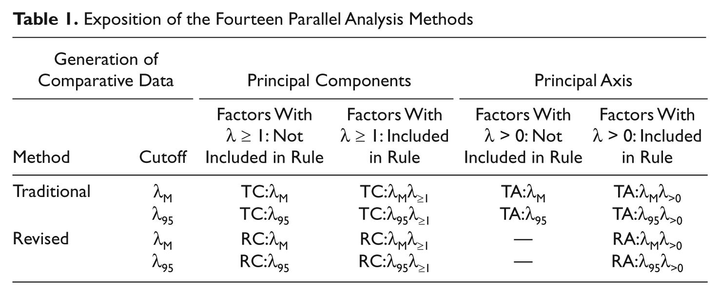
The primary goal of our Monte Carlo study was to evaluate the relative accuracy of revised and traditional parallel analysis methods. These methods are applied using a number of variations; the 14 variations are shown in Table 1. More specifically, for both traditional and revised parallel analyses, we applied two eigenvalue rules: (a) the eigenvalue for the observed data set must exceed the 95th percentile of the eigenvalues from the comparative data sets (λ₉₅ rule) and (b) the eigenvalue for the observed data set must exceed the mean of the eigenvalues from the comparative data sets (λ_M rule). In addition, we considered parallel analyses using principal component analysis and principal axis factoring. Finally, we included or excluded in our parallel analysis methods a cutoff on eigenvalues of 0 for principal axis factoring and 1.0 for principal component analyses. For the revised parallel analysis method based on principal axis factoring, however, we always required eigenvalues to be greater than 0 to avoid the nonsensical step of generating comparative data based on a factor with zero or negative variance.

Table 1.

Exposition of the Fourteen Parallel Analysis Methods

Generation of Comparative Data		Principal Components		Principal Axis
Method	Cutoff	Factors With λ ≥ 1: Not Included in Rule	Factors With λ ≥ 1: Included in Rule	Factors With λ > 0: Not Included in Rule	Factors With λ > 0: Included in Rule
Traditional	λ_M	TC:λ_M	TC:λ_Mλ_≥1	TA:λ_M	TA:λ_Mλ_>0
	λ₉₅	TC:λ₉₅	TC:λ₉₅λ_≥1	TA:λ₉₅	TA:λ₉₅λ_>0
Revised	λ_M	RC:λ_M	RC:λ_Mλ_≥1	—	RA:λ_Mλ_>0
	λ₉₅	RC:λ₉₅	RC:λ₉₅λ_≥1	—	RA:λ₉₅λ_>0

Method

In this section, we describe the variables manipulated in the generation of the data, the method used to generate the sample data and the data for the parallel analyses, and the analyses to assess the number of factors.

Data Generation Design

The data generation design included 90 conditions as a function of five manipulated variables:

Number of observations (N_O): The number of observations was set at 100, 300, or 500.

Number of factors (N_F): Data were generated based on factor models with 0, 1, 2, or 3 factors.

Number of variables (N_V): For data generated based on 0 factors or 1 factor, the number of variables was either 6 or 12. For data generated based on a model with 2 or 3 underlying factors, any variable had a nonzero loading on one and only one factor, and the number of variables with nonzero loadings was either 3 or 6 per factor. Accordingly, N_V was 6 or 12 for 0, 1, or 2 factor models and 9 or 18 for 3 factor models.

Factor loadings: The nonzero loadings for data generated with 1 or more factors were all .4 or all .7.

Factor correlations: The factor correlations for data generated with 2 or 3 factors were 0, .5, or .8.

Data Generation

One thousand data sets representing the sample data were generated for each condition based on Equation (1). For data sets with uncorrelated factors, the scores for each factor in F were generated using RANNOR, an SAS normal random number generator, with a mean of zero and a unit variance. For data sets with correlated factors, the scores for factors were generated based on a higher-order factor structure, specified to create the desired correlation among the factors of interest. The scores for these higher-order factors and the disturbances to create the factors of interest were generated using RANNOR. Finally, the error scores in E were generated using RANNOR, the errors for the measured variables were specified to be uncorrelated with each other and the factor scores, and the variances of the errors were set such that the variances of the measured variables in X were unities.

For traditional parallel analysis, 100 data sets were generated for each of the 1,000 sample data sets. These 100 data sets had the same number of variables and observations as the sample data and were generated using RANNOR. The variables were specified to be normally distributed, with means of zero, unit variances, and zero correlations with each other. For revised parallel analysis, 100 data sets were generated to assess each sequential eigenvalue associated with a sample data set. The generation of the data sets for revised parallel analysis followed the procedures previously described in the section titled “The Revised Parallel Analysis Method.” RANNOR was used to generate the normally distributed scores for the comparison data sets.

Data Analysis

Each of the 1,000 sample data sets and their accompanying comparative data sets were analyzed using the 14 methods shown in Table 1. When principal axis factoring was applied in conducting parallel analyses, the communalities were sample multiple R²s between the variables and all remaining variables in the data set. To abbreviate the otherwise unwieldy names of the methods, the approach to parallel analysis is abbreviated as T (traditional) or R (revised) and the extraction method is abbreviated as C (component analysis) or A (axis factoring). Subscripts following λ indicate the rule used. For example, revised parallel analysis using principal component analysis and implementing the 95th percentile rule with eigenvalues greater than or equal to 1 is abbreviated as RC:λ₉₅λ_≥1.

To assess the quality of a parallel analysis method for a condition, we computed the percentage of replications with the correct number of identified factors. We also assessed whether there was a tendency for a method to assess too few factors (underfactoring) or too many factors (overfactoring). Arbitrarily, we noted a tendency to underfactor if the percentage of replications yielding too few factors was 5% or more, and this percentage was at least 5% greater than the percentage of replications yielding too many factors. Similarly, we indicated a tendency to overfactor if the percentage of replications yielding too many factors was 5% or more, and this percentage was at least 5% greater than the percentage of replications yielding too few factors.

We also evaluated a method’s overall quality by appraising whether its accuracy was well behaved across conditions. More specifically, a method should demonstrate greater accuracy as sample size increases. In addition, accuracy should increase as factors are better defined, that is, as the magnitude of factor loadings increases and as the number of items assessing a factor increases. Finally, a method should show some decrement in accuracy as factors become highly correlated in that they become less distinct.

It should be noted that, ideally, accuracy for methods using the λ₉₅ rule should approach but not exceed 95%. For data with k factors, these methods could potentially be 100% accurate in identifying the presence of the 1st through kth factor, but should be at most 95% accurate in identifying the absence of the kth + 1 factor.

Results

We initially consider whether the inclusion of an absolute eigenvalue cutoff improves the accuracy of parallel analyses. We then compare revised and traditional parallel analysis methods.

Assessment of Inclusion of Absolute Eigenvalue Cutoffs in Parallel Analyses

We compared parallel analysis methods with and without the addition of absolute eigenvalue cutoffs of 0 for principal axis factoring (λ > 0 cutoff) and greater than or equal to 1 for principal component analysis (denoted λ ≥ 1 cutoff). Across all conditions, we found no differences in accuracies between the traditional methods with or without absolute eigenvalue cutoffs, regardless of whether principal component analysis or principal axis factoring in combination with λ_M rule or λ₉₅ rule was applied; accordingly, we present in tables only those results for traditional methods with the appropriate absolute eigenvalue cutoff.

In contrast, inclusion of the λ ≥ 1 cutoff tended to affect the accuracy of revised parallel analysis using principal component analysis, regardless of whether λ_M rule or λ₉₅ rule was applied. In Tables 2 and 3, we present results for a subset of the conditions to illustrate these effects. Inclusion of the λ ≥ 1 cutoff had no effect with zero underlying factors and a neutral or positive effect with one or more uncorrelated factors. In some conditions, these effects were very strong, with percentages increasing from 0 without the λ ≥ 1 cutoff to 100 with the cutoff. With 2 or 3 moderately correlated (i.e., .5) underlying factors, similar results were found, with only three minor exceptions. In contrast, for conditions with highly correlated factors (i.e., .8), inclusion of the λ ≥ 1 cutoff frequently produced negative effects. In some of these conditions, accuracy decreased with increases in sample size when the λ ≥ 1 absolute cutoff was applied.

Table 2.

Accuracy Percentages for Revised Parallel Analysis Based on Principal Components for Conditions With Zero or One Underlying Factor

		6 Variables				12 Variables
		95th Percentile Eigenvalue		Mean Eigenvalue Rule		95th Percentile Eigenvalue		Mean Eigenvalue Rule
Sample Size	Factor Loadings	RC:λ₉₅	RC:λ₉₅λ_≥1	RC:λ_M	RC:λ_Mλ_≥1	RC:λ₉₅	RC:λ₉₅λ_≥1	RC:λ_M	RC:λ_Mλ_≥1
Zero underlying factors
100	—	94.6^O	94.6^O	50.8^O	50.8^O	93.4^O	93.4^O	52.2^O	52.2^O
300	—	95.1^O	95.1	55.5^O	55.5^O	94.7^O	94.7^O	53.6^O	53.6^O
500	—	94.2^O	94.2^O	55.2^O	55.2^O	94.9^O	94.9^O	54.8^O	54.8^O
One underlying factor
100	.4	58.6^O	58.6^O	2.7^O	13.2^O	81.4^O	81.4^O	16.1^O	16.1^O
	.7	78.8^O	100.0	1.3^O	100.0	95.4	99.1	20.5^O	98.6
300	.4	7.8^O	67.3^O	0.0^O	66.8^O	53.6^O	53.6^O	3.1^O	3.3^O
	.7	14.1^O	100.0	0.0^O	100.0	80.4^O	100.0	2.8^O	100.0
500	.4	0.0^O	90.7^O	0.0^O	90.7^O	31.5^O	31.5^O	.3^O	5.3^O
	.7	0.2^O	100.0	0.0^O	100.0	62.2^O	100.0	.4^O	100.0

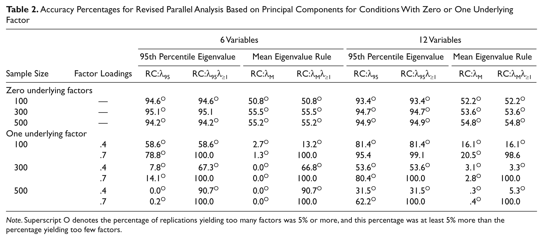
Note. Superscript O denotes the percentage of replications yielding too many factors was 5% or more, and this percentage was at least 5% more than the percentage yielding too few factors.

Table 3.

Accuracy Percentages for Revised Parallel Analysis Based on Principal Components for Conditions With Two and Three Underlying Factors

		3 Variables Per Factor				6 Variables Per Factor
		95th Percentile Eigenvalue		Mean Eigenvalue Rule		95th Percentile Eigenvalue		Mean Eigenvalue Rule
Sample Size	Factor Loadings	RC:λ₉₅	RC:λ₉₅λ_≥1	RC:λ_M	RC:λ_Mλ_≥1	RC:λ₉₅	RC:λ₉₅λ_≥1	RC:λ_M	RC:λ_Mλ_≥1
Correlation of 0 between two factors
100	.4	24.2^U	30.5^U	0.2^O	42.9^O	71.9^O	71.9^O	12.0^O	12.0^O
	.7	99.8	100.0	95.7	100.0	100.0	100.0	99.6	99.8
300	.4	4.9^O	86.4^O	0.0^O	87.0^O	47.5^O	47.5^O	0.9^O	1.5^O
	.7	100.0	100.0	100.0	100.0	100.0	100.0	100.0	100.0
500	.4	0.5^O	98.1	0.0^O	98.1	28.8^O	30.0^O	0.2^O	15.9^O
	.7	100.0	100.0	100.0	100.0	100.0	100.0	100.0	100.0
Correlation of .8 between two factors
100	.4	21.6^U	32.2^U	0.0^O	68.6^O	23.1^U	23.1^U	11.2^O	11.2^O
	.7	77.3^U	8.9^U	25.3^O	8.9^U	91.9^U	87.0^U	65.4^O	88.4^U
300	.4	0.0^O	60.0^U	0.0^O	60.9^U	25.2^O	25.2^O	0.1^O	3.6^U
	.7	89.6^O	0.2^U	11.9^O	0.2^U	99.7	91.9^U	67.5^O	91.9^U
500	.4	0.0^O	33.9^U	0.0^O	33.9^U	9.5^O	24.7^O	0.0^O	25.9^O
	.7	82.5^O	0.0^U	6.4^O	0.0^U	99.6	94.6^U	71.0^O	94.6^U
Correlation of 0 among 3 factors
100	.4	16.1^U	16.1^U	1.3^O	18.8^O	59.2^U	59.2^U	14.3^O	14.3^O
	.7	100.0	100.0	99.4	100.0	100.0	100.0	100.0	100.0
300	.4	9.1^O	57.3^O	0.0^O	57.6^O	57.9^O	57.9^O	3.5^O	3.5^O
	.7	100.0	100.0	100.0	100.0	100.0	100.0	100.0	100.0
500	.4	1.0^O	85.4^O	0.0^O	85.4^O	40.3^O	40.3^O	0.8^O	0.8^O
	.7	100.0	100.0	100.0	100.0	100.0	100.0	100.0	100.0
Correlation of .8 among 3 factors
100	.4	6.0^U	6.1^U	2.2^O	51.6^O	3.1^U	3.1^U	15.6^O	15.6^O
	.7	9.6^U	1.3^U	61.5^O	1.3^U	43.6^U	43.6^U	81.4	77.4^U
300	.4	4.6^O	42.0^U	0.0^O	53.1^U	13.1^U	13.1^U	3.1^O	3.1^O
	.7	92.2^U	0.0^U	65.1^O	0.0^U	100.0	80.9^U	94.1^O	80.9^U
500	.4	0.0^O	20.9^U	0.0^O	21.6^U	17.9	17.9	1.0^O	0.2^O
	.7	99.0	0.0^U	67.6^O	0.0^U	100.0	87.6^U	97.6	87.6^U

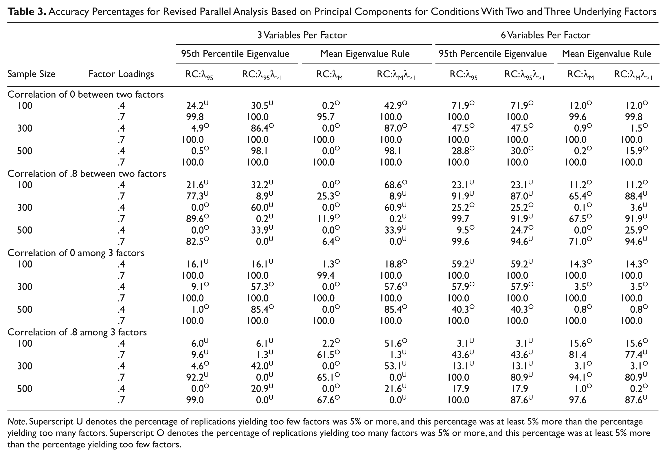
Note. Superscript U denotes the percentage of replications yielding too few factors was 5% or more, and this percentage was at least 5% more than the percentage yielding too many factors. Superscript O denotes the percentage of replications yielding too many factors was 5% or more, and this percentage was at least 5% more than the percentage yielding too few factors.

Overall, inclusion of the λ ≥ 1 absolute cutoff tended to improve performance of the revised parallel analysis method using principal component analysis. More specifically, inclusion of the λ ≥ 1 absolute cutoff produced no improvement for zero underlying factors, marked improvement for many conditions with one underlying factor, and improvement in many conditions with two or three underlying factors, except when factors were highly correlated.

Comparison of Revised Versus Traditional Parallel Analysis Methods

We present the accuracy percentages for assessing the relative quality of the revised and traditional parallel analysis methods for zero and one underlying factor in Table 4 and for two and three underlying factors in Figures 2 and 3, respectively. In the table and figures, we included the absolute eigenvalue cutoff of 1 as part of the revised methods using principal component analysis because it tended to produce more accurate results, as discussed in the previous section. For simplicity, we labeled the accuracy percentages for the traditional methods as including the absolute eigenvalue cutoffs of 0 or 1, although the same accuracy percentages were found for traditional methods that did not include these cutoffs. We discuss results separately for conditions with 0, 1, and 2 or more underlying factors.

Table 4.

Accuracy Percentages for Traditional and Revised Parallel Analyses for Conditions With Zero or One Underlying Factor

		95th Percentile Eigenvalue Rule				Mean Eigenvalue Rule
		Principal Axis		Principal Components		Principal Axis		Principal Components
Sample Size	Factor Loadings	TA:λ₉₅λ_>0	RA:λ₉₅λ_>0	TC:λ₉₅λ_≥1	RC:λ₉₅λ_≥1	TA:λ_Mλ_>0	RA:λ_Mλ_>0	TC:λ_Mλ_≥1	RC:λ_Mλ_≥1
Zero underlying factors—6 variables
100	—	95.1	95.1	94.6^O	94.6^O	51.9^O	51.9^O	50.8^O	50.8^O
300	—	95.1	95.1	95.1	95.1	55.5^O	55.5^O	55.5^O	55.5^O
500	—	94.3^O	94.3^O	94.2^O	94.2^O	55.3^O	55.3^O	55.2^O	55.2^O
Zero underlying factors—12 variables
100	—	94.1	94.1	93.4	93.4^O	53.6^O	53.6^O	52.2^O	52.2^O
300	—	94.7	94.7	94.7	94.7^O	53.8^O	53.8^O	53.6^O	53.6^O
500	—	94.9	94.9	94.9	94.9^O	54.1^O	54.1^O	54.8^O	54.8^O
One underlying factor—6 variables
100	.4	92.9	94.1	96.7	58.6^O	63.2^O	57.7^O	86.3^O	13.2^O
	.7	100.0	96.2	100.0	100.0	98.2	59.5^O	100.0	100.0
300	.4	98.2	97.0	99.8	67.3^O	87.5^O	63.7^O	99.2	66.8^O
	.7	100.0	96.0	100.0	100.0	100.0	59.8^O	100.0	100.0
500	.4	99.9	96.8	100.0	90.7^O	94.2^O	64.3^O	100.0	90.7^O
	.7	100.0	96.2	100.0	100.0	100.0	81.8^O	100.0	100.0
One underlying factor—12 variables
100	.4	94.1^O	94.7^O	99.0	81.4^O	64.8^O	53.8^O	88.8^O	16.1^O
	.7	100.0	97.1	100.0	99.1	100.0	56.3^O	100.0	98.6
300	.4	98.2	95.0^O	100.0	53.6^O	81.1^O	54.8^O	99.6	3.3^O
	.7	100.0	95.4	100.0	100.0	100.0	56.0^O	100.0	100.0
500	.4	99.6	96.0	100.0	31.5^O	89.6^O	56.5^O	100.0	5.3^O
	.7	100.0	96.3	100.0	100.0	100.0	55.8^O	100.0	100.0

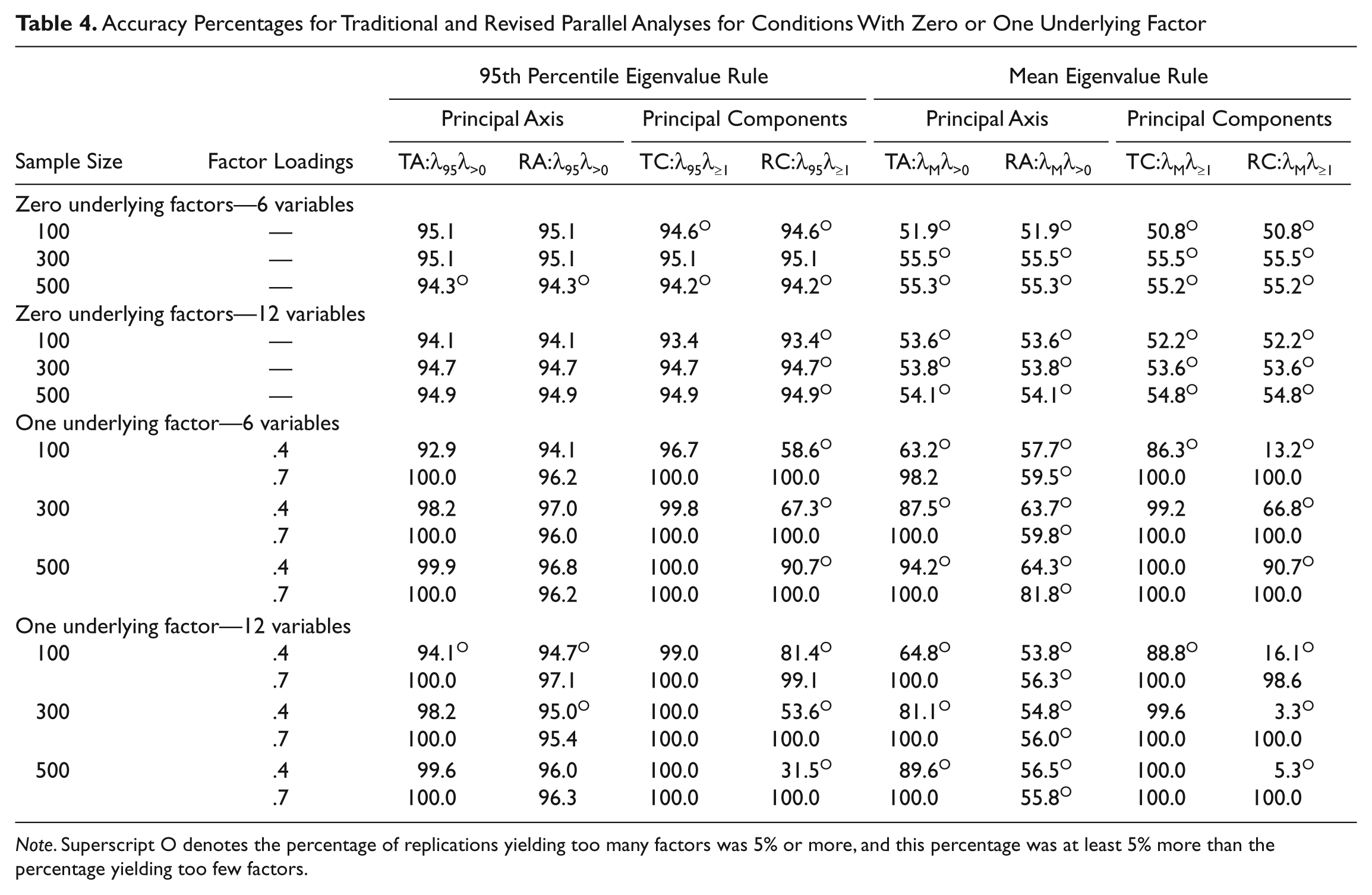
Note. Superscript O denotes the percentage of replications yielding too many factors was 5% or more, and this percentage was at least 5% more than the percentage yielding too few factors.

Figure 2.

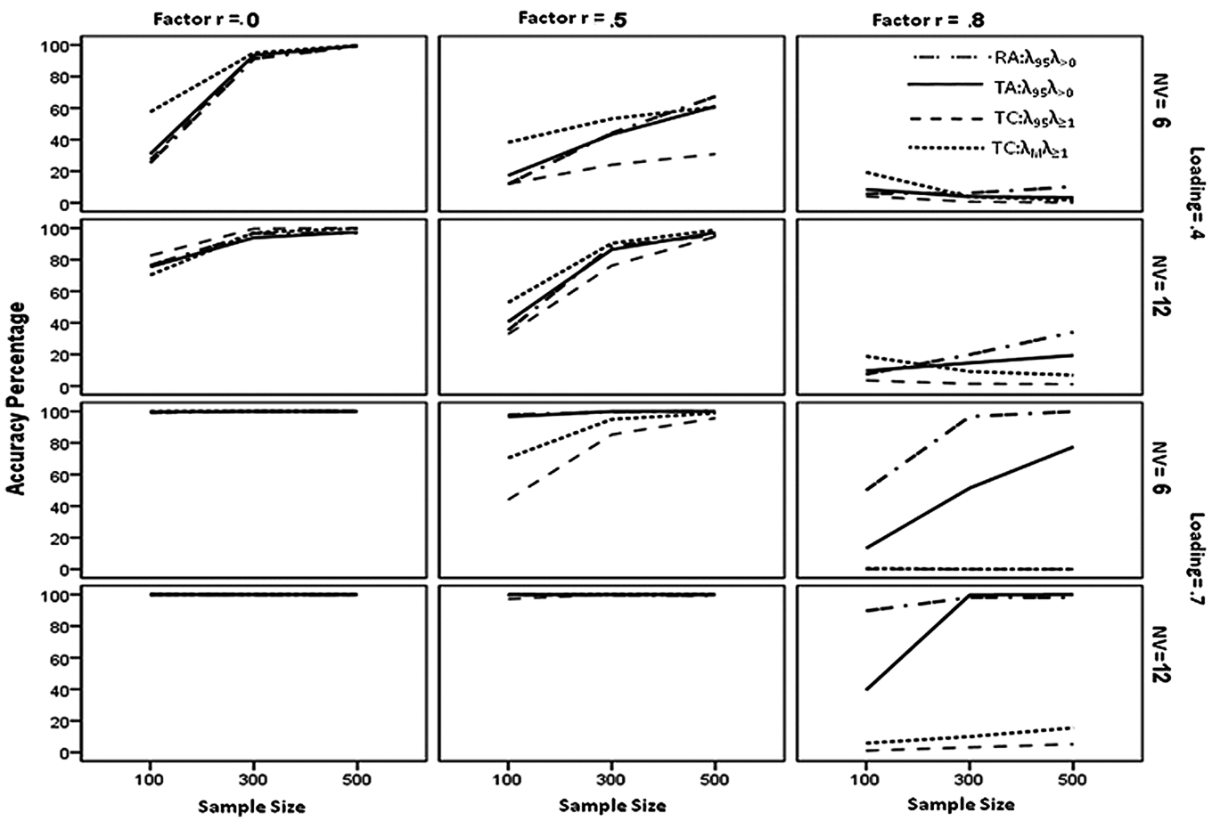
Accuracy of four parallel analysis methods for conditions with two underlying factors. Note that the lines for TC:λ₉₅λ_≥1 and TC:λ_Mλ_≥1 are superimposed on each other and evidence near zero accuracy for the next to the last graph in the third column.

Figure 3.

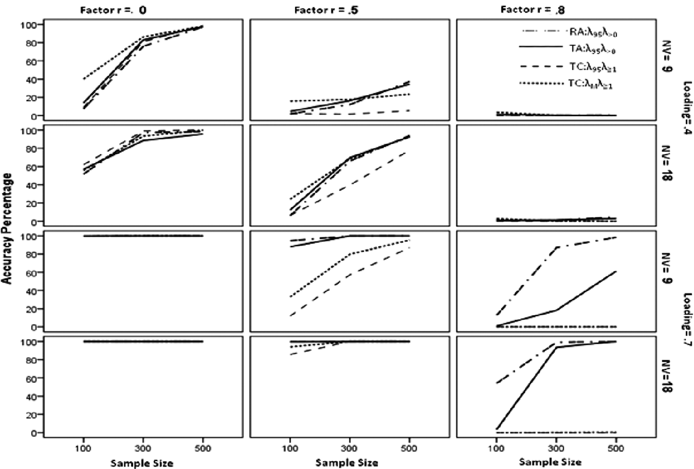
Accuracy of four parallel analysis methods for conditions with three underlying factors. Note that the lines for TC:λ₉₅λ_≥1 and TC:λ_Mλ_≥1 are superimposed on each other and evidence near zero accuracy for the bottom two graphs in the third column

No underlying factors

For conditions with 0 underlying factors, as shown in Table 4, the traditional and revised parallel analysis methods produced equivalent results. The major differences in accuracy across all methods occurred between methods that used the λ₉₅ rule (percentages between 93.4 and 95.1) and those that used the λ_M rule (percentages between 50.8 and 55.5).

One underlying factor

As presented in Table 4 for conditions with one underlying factor, traditional parallel analysis tended to yield similar or higher accuracy percentages in comparison with comparable revised methods. However, the differences between the revised and the traditional approaches were minimal for principal axis factoring with the 95th percentile eigenvalue rule. Overall, the accuracies for parallel analysis methods using the 95th percentile eigenvalue rule were equal to or greater than the accuracies for comparable methods using the mean eigenvalue rule. Of the methods using the 95th percentile eigenvalue rule, the revised method based on principal component analysis tended to perform poorer across conditions when factor loadings were .4. For conditions with one underlying factor and loadings of .7, accuracy always exceeded 95%.

Two or three underlying factors

We present the accuracy percentages for parallel analysis methods to detect two and three underlying factors in Figures 2 and 3, respectively. Only four of the parallel analysis methods—TA:λ₉₅λ_>0, RA:λ₉₅λ_>0, TC:λ₉₅λ_≥1, and TC:λ_Mλ_≥1—were included on the graphs to make them less cluttered and easier to interpret.

The accuracies for the four methods excluded from the graphs—RC:λ₉₅λ_≥1, TA:λ_Mλ_>0, RA:λ_Mλ_>0, and RC:λ_Mλ_≥1—behaved poorly for data with two and three underlying factors. In particular, the accuracies for RC:λ₉₅λ_≥1 and RC:λ_Mλ_≥1 often failed to increase with increases in sample size (holding other manipulated dimensions constant). The insensitivity to sample size occurred across a wide variety of conditions: 2 or 3 underlying factors; correlations among factors of 0, .5, or .8; and 3 or 6 variables per factor. In addition, these two methods frequently showed decreases in accuracy with increases in the number of variables per factor when loadings were .4, holding all other manipulated dimensions constant. Finally, the accuracies for RC:λ₉₅λ_≥1 and RC:λ_Mλ_≥1 commonly increased in value as the correlation between factors increased from 0 to .5. The accuracies for the other two methods excluded from the graphs (TA:λ_Mλ_>0 or RA:λ_Mλ_>0) also behaved badly. The accuracies for TA:λ_Mλ_>0 decreased in value with increases in sample size when factors were correlated .8, the number of variables per factor was 3, and the factor loadings were .4. Multiple times the percentages for RA:λ_Mλ_>0 remained relatively homogeneous or decreased in value with increases in sample size across conditions with all other manipulated factors held constant. These results were particularly difficult to understand in that they occurred only across conditions in which factors were relatively well defined, that is, those with 6 variables per factor and factor loadings of .7. Last, the accuracies for both TA:λ_Mλ_>0 and RA:λ_Mλ_>0 often decreased in value with increases in the number of variables per factor.

We now turn our attention to Figures 2 and 3. No single method shown in these figures yielded consistently more accurate results across all conditions. All four methods produced very accurate results with high factor loadings and uncorrelated factors (i.e., bottom two graphs on left side in Figures 2 and 3) and inaccurate results with low factor loadings and highly correlated factors (i.e., top two graphs on right side in Figures 2 and 3).

The parallel analysis methods using principal component analyses tended overall to perform more poorly. Although the accuracies for TC:λ₉₅λ_≥1 were similar to those for the other three methods when factors were uncorrelated, they generally had the lowest values when factors were correlated .5 or .8. The accuracy percentages for TC:λ_Mλ_≥1 were highest among the four methods under some conditions (e.g., N = 100, 2 factors correlated .5 or .8, factor loadings of .4) and approached zero under others (e.g., 2 factors correlated .8, factor loadings of .7, and 3 variables per factor). In addition, as shown in the top two graphs in the last column of Figure 2, the accuracies for TC:λ_Mλ_≥1 were badly behaved when factors were correlated .8 in that the accuracies for TC:λ_Mλ_≥1 decreased with increases in sample size.

The accuracies for TA:λ₉₅λ_>0 and RA:λ₉₅λ_>0 were generally well behaved. The only exceptions were for conditions with highly correlated factors, weak factor loadings, and three variables per factor. For these conditions, the accuracies for TA:λ₉₅λ_>0 were generally low and decreased in value with increases in sample size (from 8.5 to 3.4 and from 1.2 to .1 for 2 and 3 underlying factors, respectively). On the other hand, the accuracies for RA:λ₉₅λ_>0 for these conditions properly increased in values (from 5.7 to 10.2) with increases in sample size with 2 underlying factors, but were homogeneous and very low (between .3 and .6) with 3 underlying factors. Across conditions, RA:λ₉₅λ_>0 generally was approximately as accurate or more accurate than TA:λ₉₅λ_>0.

Discussion

We could make the following recommendation based on the results: (a) any of the methods that use the 95th percentile rule are effective in assessing 0 underlying factors; (b) TC:λ₉₅λ_≥1 is most effective in evaluating 1 underlying factor; (c) TC:λ_Mλ_≥1 works best with multiple uncorrelated factors with 3 variables per factor; (d) TC:λ₉₅λ_≥1 is preferred with multiple uncorrelated factors with 6 variables per factor; (e) RC:λ_Mλ_≥1 yields the best results for moderately correlated factors with 3 variables per factor; (f) TC:λ_Mλ_≥1 produces the best results for moderately correlated factors with 6 variables per factor; (g) RC:λ_Mλ_≥1 had the highest accuracies for highly correlated factors with 3 variables per factor and low factor loadings; (h) RA:λ_Mλ_>0 had the highest accuracies for highly correlated factors with 6 variables per factor and low factor loadings; (i) RA:λ₉₅λ_>0 tends to work best across conditions for highly correlated factors with high factor loadings if the sample size is 300 or greater; (j) RC:λ₉₅ is preferred for two highly correlated factors with high factor loadings if the sample size is 100; and (k) RC:λ_M yields the best results for three highly correlated factors with high factor loadings if the sample size is 100.

At this point, readers are likely to be wondering what to make of recommendations of seven different methods dependent on conditions of a study. In practice, researchers who apply parallel analysis know the basic design of their study: the number of subjects and the number of variables in their study. However, they do not know the number of factors underlying their measures, the number of variables associated with each factor, the correlation among factors, and the magnitudes of the factor loadings. Accordingly, researchers need a parallel analysis method that is relatively accurate across different factor structures.

On the whole, the revised parallel analysis method based on principal axis factoring using the λ₉₅ rule (RA:λ₉₅λ_>0) yielded relatively high accuracy percentages in comparison with other methods across various factor structures. With zero or one underlying factor, the accuracy percentages for this method were greater than 94%. For conditions with two or three factors, the accuracies for RA:λ₉₅λ_>0 were excellent (i.e., mean of 94%) when factor loadings were high and fair when factor loadings were low as long as samples were at least moderate in size (i.e., mean of 50% with N = 300 and mean of 61% with N = 500).

The finding that percentages for RA:λ₉₅λ_>0 tended to perform better than other parallel analysis methods with well-defined factor structures is consistent with the conceptual underpinning of these methods in two ways. First, the data were generated using a common factor model, and therefore parallel analysis methods using this model, such as principal axis factoring, should produce more orderly results than those based on a principal component model. Second, the revised method uses factor loadings from the observed data to generate the comparison data sets. These factor loadings are likely to yield more stable and accurate results for studies with large sample sizes and factor structures with high factor loadings and many variables per factor. Accordingly, RA:λ₉₅λ_>0 should be and was most accurate with a sample size of 500, factor loadings of .7, and 6 variables per factor (accuracies across these conditions of 98% or greater). From a practical viewpoint, the results suggest researchers are more likely to identify correctly a two- or three-factor model using RA:λ₉₅λ_>0 if they have well-designed measures and studies. In other words, the use of this method reinforces good research practices.

Our study also indicated that the inclusion of an absolute eigenvalue cutoff of 0 for principal axis factoring or 1 for principal component analysis had no effect on traditional parallel analysis and a positive effect on revised parallel analysis. Based on the results for the traditional parallel analysis methods, the eigenvalue-greater-than-one criterion does not produce fewer factors than traditional parallel analysis methods. This finding is consistent with previous research that suggests that the eigenvalue-greater-than-one criterion overfactors and performs poorly in comparison with parallel analysis methods (e.g., Zwick & Velicer, 1986).

In summary, the revised parallel analysis method using principal axis factoring and the 95th percentile rule offers promise based on the findings of our investigation. Future research should include additional conditions with more varied factor structures to ensure the generality of our conclusion.

Footnotes

The author(s) declared no potential conflicts of interest with respect to the research, authorship, and/or publication of this article.

The author(s) received no financial support for the research, authorship, and/or publication of this article.

References

Buja

Eyuboglu

(1992). Remarks on parallel analysis. Multivariate Behavioral Research, 27, 509-540.

Cattell

R. B.

(1978). The scientific use of factor analysis in behavioral and life sciences. New York, NY: Plenum.

Crawford

Green

S. B.

Levy

W.-J.

Scott

Svetina

D. S.

Thompson

M. S.

(2010). Evaluation of parallel analysis methods for determining the number of factors. Educational and Psychological Measurement, 70, 885-901.

Fabrigar

L. R.

Wegener

D. T.

MacCallum

R. C.

Strahan

E. J.

(1999). Evaluating the use of exploratory factor analysis in psychological research. Psychological Methods, 4, 272-299.

Ford

J. K.

MacCallum

R. C.

Tait

(1986). The applications of exploratory factor analysis in applied psychology: A critical review and analysis. Personnel Psychology, 39, 291-314.

Glorfeld

L. W.

(1995). An improvement on Horn’s parallel analysis methodology for selecting the correct number of factors to retain. Educational and Psychological Measurement, 55, 377-393.

Guttman

(1954). Some necessary conditions for common factor analysis. Psychometrika, 19, 149-161.

Harshman

R. A.

Reddon

J. R.

(1983). Determining the number of factors by comparing real with random data: A serious flaw and some possible corrections. Proceedings of the Classification Society of North America at Philadelphia, 14-15.

Horn

J. L.

(1965). A rationale and test for the number of factors in factor analysis. Psychometrika, 30, 179-185.

10.

Humphreys

L. G.

Montanelli

R. G.

(1975). An investigation of the parallel analysis criterion for determining the number of common factors. Multivariate Behavioral Research, 10, 193-206.

11.

Kaiser

H. F.

(1960). The application of electronic computers to factor analysis. Educational and Psychological Measurement, 20, 141-151.

12.

Mulaik

S. A.

(2010). Foundations of factor analysis (2nd ed.). Boca Raton, FL: Chapman & Hall/CRC.

13.

Preacher

K. J.

MacCallum

R. C.

(2003). Repairing Tom Swift’s electric factor analysis machine. Understanding Statistics, 2, 13-43.

14.

Snook

S. C.

Gorsuch

R. L.

(1989). Component analysis versus common factor analysis: A Monte Carlo study. Psychological Bulletin, 106, 148-154.

15.

Steger

M. F.

(2006). An illustration of issues in factor extraction and identification of dimensionality in psychological assessment data. Journal of Personality Assessment, 86, 263-272.

16.

Turner

N. E.

(1998). The effect of common variance and structure pattern on random data eigenvalues: Implications for the accuracy of parallel analysis. Educational and Psychological Measurement, 58, 541-568.

17.

Velicer

W. F.

Eaton

C. A.

Fava

J. L.

(2000). Construct explication through factor or component analysis: A review and evaluation of alternative procedures for determining the number of factors or components. In Goffin

R. D.

Helmes

(Eds.), Problems and solutions in human assessment: Honoring Douglas Jackson at seventy (pp. 41-71). Boston, MA: Kluwer.

18.

Widaman

K. F.

(1993). Common factor analysis versus principal component analysis: Differential bias in representing model parameters? Multivariate Behavioral Research, 28, 263-311.

19.

Zwick

W. R.

Velicer

W. F.

(1986). Comparison of five rules for determining the number of components to retain. Psychological Bulletin, 99, 432-442.