The Rasch Rating Model and the Disordered Threshold Controversy

Abstract

The Rasch rating (or partial credit) model is a widely applied item response model that is used to model ordinal observed variables that are assumed to collectively reflect a common latent variable. In the application of the model there is considerable controversy surrounding the assessment of fit. This controversy is most notable when the set of parameters that are associated with the categories of an item have estimates that are not ordered in value in the same order as the categories. Some consider this disordering to be inconsistent with the intended order of the response categories in a variable and often term it reversed deltas. This article examines a variety of derivations of the model to illuminate the controversy. The examination of the derivations shows that the so-called parameter disorder and order of the response categories are separate phenomena. When the data fit the Rasch rating model the response categories are ordered regardless of the (order of the) values of the parameter estimates. In summary, reversed deltas are not necessarily evidence of a problem. In fact the reversed deltas phenomenon is indicative of specific patterns in the relative numbers of respondents in each category. When there are preferences about such relative numbers in categories, the patterns of deltas may be a useful diagnostic.

Keywords

partial credit model Rasch model Rasch rating model

The Rasch rating (or partial credit) model (Andrich, 1978; Masters, 1982) is a widely applied item response model that is used to model ordinal variables that are assumed to collectively reflect a common latent variable.

In the application of the model there is considerable controversy in relation to the practical implications of situations where the set of parameters that are associated with the categories of an item have estimates that are not ordered in value. Some consider this phenomenon to be inconsistent with the intended order of the response categories in a variable and often term it either disordered thresholds or reversed deltas.

The view that estimated parameter disorder represents an incompatibility of the data with the underlying measurement intentions of Rasch measurement has been strongly advocated by Andrich (1978, 2005) and is embodied in Andrich’s computer program, RUMM2020 (Andrich, Sheridan, & Luo, 2003), which routinely alerts users to this as a problem. Furthermore, in a number of applied settings disorder of estimated parameters has been used as evidence of a problem with the intended ordering of the response categories (e.g., Nijsten, Sampogna, Chren, & Abeni, 2006; Nilsson, Sunnerhagen, & Grimby, 2007; Zhu, Timm, & Ainsworth, 2001).

Other model and software developers, however, do not see disorder of estimated parameter as a violation of the intended order of the response categories in items (e.g., Linacre, 1991; Masters, 1982). They argue that while there are certainly circumstances under which disorder of estimated parameter may be reflective of a flaw in the measurement instrument, they neither see disorder of estimated parameter necessarily as an indicator of misfit of data to the model nor as an indicator of underlying category disorder.

In this article, we review presentations and derivations of the model that have been provided by Andersen (1973), Fischer (1995), Andrich (1978, 2005), and Masters (1980) and discuss the relationship between the model parameters and the ordering of Rasch rating model categories. In the next section, we present alternative formulations of the model and discuss the relationships among their parameters. Then we discuss derivations of the model, particularly that of Andrich (1978, 2005), and in doing so review the relationship between category order and the order of the model parameters. We then provide two formal definitions of order and show that the Rasch rating model satisfies these definitions regardless of the values of the parameters. Then we examine parameter estimation and show that for any given set of abilities the relative frequency of the number of responses in each category of an item is the only determinant of whether the estimated parameters are ordered in value or not. We then consider some alternative models to the Rasch rating model and finally we discuss the application of the Rasch rating model to sets of binary items that conform to the simple logistic model.

The Rasch Rating Model

The Rasch model for polytomous items has been presented in the literature in a variety of different forms. The first presentation of the model was most likely that of Rasch (1961), whereas those of Andersen (1977), Andrich (1978), and Masters (1982) are now commonly used.

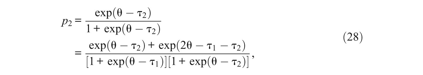
If we let X_ni be the response of individual n on item i, then, following Andersen (1977), the probability of a response k, k = 0, …,m, is

P (X_{ni} = k) = \frac{\exp (φ_{k} θ_{n} - β_{ik})}{\sum_{t = 0}^{m} \exp (φ_{t} θ_{n} - β_{it})} .

In (1), φ_k are scoring functions for the categories, θ_n is the person parameter, and β_ik is a parameter that describes the relative attractiveness of category k of item i. Throughout this discussion we will consider the case where the scoring functions are given by φ_k = k so that (1) becomes

P (X_{ni} = k) = \frac{\exp (k θ_{n} - β_{ik})}{\sum_{t = 0}^{m} \exp (t θ_{n} - β_{it})} .

Andrich (1978) expressed the same model in the following form¹:

P (X_{ni} = k) = \frac{1}{γ_{ni}} \exp (\sum_{t = 0}^{k} τ_{it} + k (θ_{n} - δ_{i})) .

In (3), $τ_{i 0} \equiv 0$ , $\sum_{t = 0}^{m} τ_{it} = 0,$ and γ_ni is a normalizing factor. Andrich refers to the δ (delta) parameter as the item location parameter and the τ (tau) parameters as thresholds. The reasoning behind this is discussed in the derivation below. Throughout this article, we shall refer to them as the tau parameters.

Masters (1982) expressed the same model in the following form:

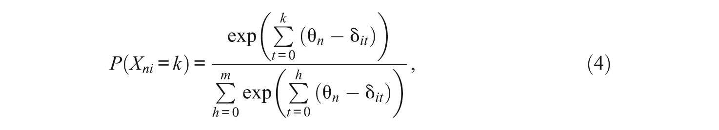
P (X_{ni} = k) = \frac{\exp (\sum_{t = 0}^{k} (θ_{n} - δ_{it}))}{\sum_{h = 0}^{m} \exp (\sum_{t = 0}^{h} (θ_{n} - δ_{it}))},

where, for notational convenience,

\sum_{k = 0}^{0} (θ_{j} - δ_{ik}) \equiv 0 and \sum_{k = 0}^{h} (θ_{j} - δ_{ik}) \equiv \sum_{k = 1}^{h} (θ_{j} - δ_{ik}) .

The equivalence of models given by (2), (3), and (4) is quite easy to show mathematically. The relationships between the parameters of the Andrich and Masters formulation are best illustrated graphically.

Figure 1 shows, for a hypothetical five-category item, the probabilities of a response in each of the categories as a function of the ability of person n, θn.

Figure 1.

Category characteristics curves for a five-category item

Under the Masters formulation of the model the item parameters, $δ_{ik}, k = 1, 2, 3, 4$ are the points at which $P (X_{ni} = k - 1) = P (X_{ni} = k) .$ That is, they are the intersection points of the successive pairs of category probability curves.

Under the Andrich formulation, the item difficulty parameter, δ_i, is the point at which $P (X_{ni} = 0) = P (X_{ni} = 4) .$ That is, the intersection point of the highest and lowest categories, and $τ_{ik} (k = 1, 2, 3, 4),$ are the distances between δ_i and each of the intersection points of the successive pairs of category probability curves, respectively. Furthermore, it can be shown that the Andrich item difficulty parameter, δ_i, is the average of the set of Masters item parameters.

In this particular case:

δ_{i} = \frac{1}{4} (δ_{i 1} + δ_{i 2} + δ_{i 3} + δ_{i 4})

and

\begin{matrix} τ_{i 1} = δ_{i 1} - δ_{i}, \\ τ_{i 2} = δ_{i 2} - δ_{i}, \\ τ_{i 3} = δ_{i 3} - δ_{i}, \\ τ_{i 4} = δ_{i 4} - δ_{i} . \end{matrix}

Under the Andersen formulation the parameters do not have such a simple graphical interpretation. The parameter for each category is the sum of Masters’s item parameters up to that category. That is,

β_{ik} = \sum_{t = 0}^{k} δ_{it} .

Derivations of the Model

The three formulations described in the first section were derived somewhat differently. In this section, we discuss each of those derivations, paying particular attention to the Andrich approach.

Andersen (1973) derives a general multidimensional polytomous Rasch model from the assumption that minimal sufficient statistics exist for the person parameters that are independent of the item parameters (see Fischer, 1995). The model he derives is as follows.

Consider an item with m + 1 response categories. Let $β_{i} = (β_{i 0}, \dots, β_{im})$ be a vector of item parameters for item i that describe the relative attractiveness of each response category independent of the individual. Similarly, let $θ_{vi} = (θ_{vi 0}, \dots, θ_{vim})$ be a vector of parameters that describe individual v’s predilection for choosing each response category. The multidimensional polytomous Rasch model is then defined by

\Pr (X_{vik} = 1; θ_{vi}, β_{i}) = \frac{\exp (θ_{vik} - β_{ik})}{\sum_{l = 0}^{m} \exp (θ_{vil} - β_{il})},

where X_vik are independent random variables with realizations x_vik = 1 if subject v chooses category k of item i, and x_vik = 0 otherwise.

Model (5) is more general than the Rasch rating model as given by (2), (3) and (4). The more general nature of (5) can be seen from recognizing that if the attractiveness parameter is constrained as follows: $θ_{vi} = (0, θ_{v}, 2 θ_{v}, \dots, m θ_{v}),$ then (5) becomes (2). It follows that the Rasch rating model is a unidimensional polytomous model that has minimal sufficient statistics for the person parameters that are independent of the item parameters (Fischer, 1995).

Under the assumption that items have m + 1 categorical response categories, k = 0, …, m, Fischer (1995) derives the rating form of the polytomous Rasch model from the requirement that (a) the response probability function, p(k; θ) is a continuous function, (b) that $p (k + 1; θ) / p (k + 1; θ) p (k; θ) p (k; θ)$ is strictly increasing in θ, and (c) that $p (k_{1}, k_{2} | k_{1} + k_{2} = K)$ is independent of θ. Requirement (b) is an order condition that ensures that as θ increases, the odds of observing k + 1 rather than k increases. Requirement (c) is a condition that ensures the possibility of conditional inference, this being the key requirement of Rasch models.

The Masters (1980) derivation is somewhat more heuristic. It has as its basic element an implicit specification of the order requirement in the observed responses. Masters shows that if one assumes that

\frac{p (k + 1; θ)}{p (k + 1; θ) + p (k; θ)} = \frac{\exp (θ - δ_{ik})}{1 + \exp (θ - δ_{ik})},

then the Partial Credit Model as parameterized in (4) follows.

The derivations of Andersen, Fischer, and Masters all result in a particular functional form for the model, but the authors make no comment on the ordering of the actual values of the parameters.

A fourth derivation, that of Andrich (1978, 2005), will now be discussed in more detail. Andrich argues that his derivation leads to an order requirement on the item parameters.

In what follows, the Andrich derivation of the model is described, but for reasons of simplicity this version of the derivation is restricted to the case of three response categories, and unnecessary indexing of items and students is avoided. The derivation for the general case can be found in Andrich (2005).

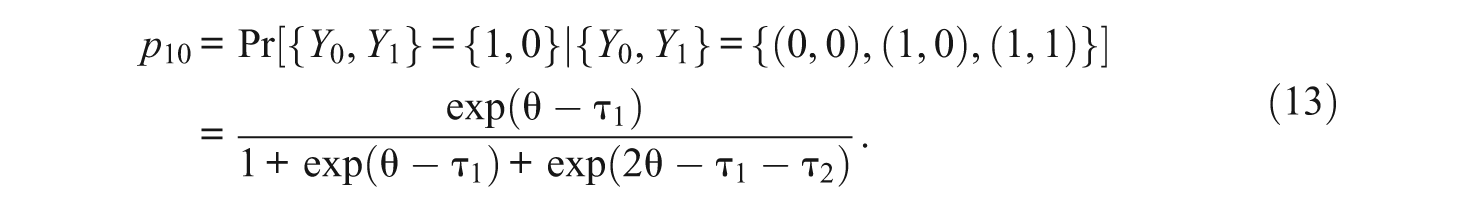
In the case of three response categories, Andrich posits an instantaneous latent response process operating at two thresholds. Letting Y_k denote the random variable that describes the outcome of the kth thresholding process, and then assuming that the probability of passing the threshold is described by the simple Rasch model, we can write

\Pr (Y_{k} = y) = \frac{\exp [y (θ_{n} - τ_{k})]}{1 + \exp (θ_{n} - τ_{k})}, y \in {0, 1}, for k = 1, 2 .

Assuming this response process, the τ_k parameters are the locations of the thresholds on the underlying scale. That is, there is a sense in which they are difficulty parameters for each of the latent response processes. This is illustrated in Figure 2, where the distributions shown are logistic distributions centered at θ_n so that the area to the right of the thresholds indicates the probability of exceeding that threshold. As plotted, the second of the two thresholds is at a higher point on the latent continuum and as such it is the more difficult of the two latent thresholds to pass. Note, however, that there is nothing in the specification of the kth thresholding process that indicates what these events, the probability of which are given by (7), are. Furthermore, there is nothing in the specification that constrains the order of the values of the τ_k parameters; they could have been reversed.

Figure 2.

Illustration of two independent logistic thresholds

Figure 3 is an extract from Andrich (1978) showing how the two latent processes were presented and labeled by Andrich, based on an item having three response categories: agree, neutral, and disagree. The presentation clearly shows that Andrich regarded the first tau parameter as a threshold between disagree and neutral or agree, whereas the second tau parameter is represented as a threshold between disagree or neutral and agree. This is not, however, what is described and depicted above, where the events are seen as independent and there is no indication of their actual meaning.

Figure 3.

Threshold process as illustrated by Andrich (1978)

If the two latent dichotomous processes were independent, four possible outcomes could occur. The probability of each of these outcomes is as follows:

\begin{matrix} {p'}_{00} = \Pr ({Y_{0}, Y_{1}} = {0, 0}) \\ = \Pr (Y_{0} = 0) \Pr (Y_{1} = 0) \\ = \frac{1}{[1 + \exp (θ - τ_{1})] [1 + \exp (θ - τ_{2})]}, \end{matrix}

\begin{matrix} {p'}_{10} = \Pr ({Y_{0}, Y_{1}} = {1, 0}) \\ = \Pr (Y_{0} = 1) \Pr (Y_{1} = 0) \\ = \frac{\exp (θ - τ_{2})}{[1 + \exp (θ - τ_{1})] [1 + \exp (θ - τ_{2})]}, \end{matrix}

\begin{matrix} {p'}_{01} = \Pr ({Y_{0}, Y_{1}} = {0, 1}) \\ = \Pr (Y_{0} = 0) \Pr (Y_{1} = 1) \\ = \frac{\exp (θ - τ_{2})}{[1 + \exp (θ - τ_{1})] [1 + \exp (θ - τ_{2})]}, \end{matrix}

\begin{matrix} {p'}_{11} = \Pr ({Y_{0}, Y_{1}} = {1, 1}) \\ = \Pr (Y_{0} = 1) \Pr (Y_{1} = 1) \\ = \frac{\exp (2 θ - τ_{1} - τ_{2})}{[1 + \exp (θ - τ_{1})] [1 + \exp (θ - τ_{2})]} . \end{matrix}

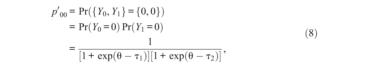
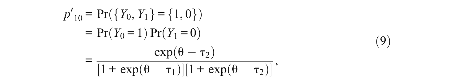
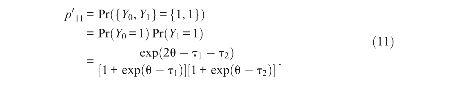
Furthermore, if it were possible to observe these four outcomes, then the model given by (8) to (11) is a special case of the ordered partition model of Wilson (1992) and Wilson and Adams (1993). It can be shown that this model is a special case of Andersen’s model as given in (5). This model can be estimated with the ConQuest software (Wu, Adams, & Wilson, 1997), and Wilson and Adams (1995) demonstrate its application to item bundles (sets of items). Furthermore, under this model the parameters τ₁ and τ₂ are thresholds on the latent continuum. The events for which they are thresholds, however, are unspecified.

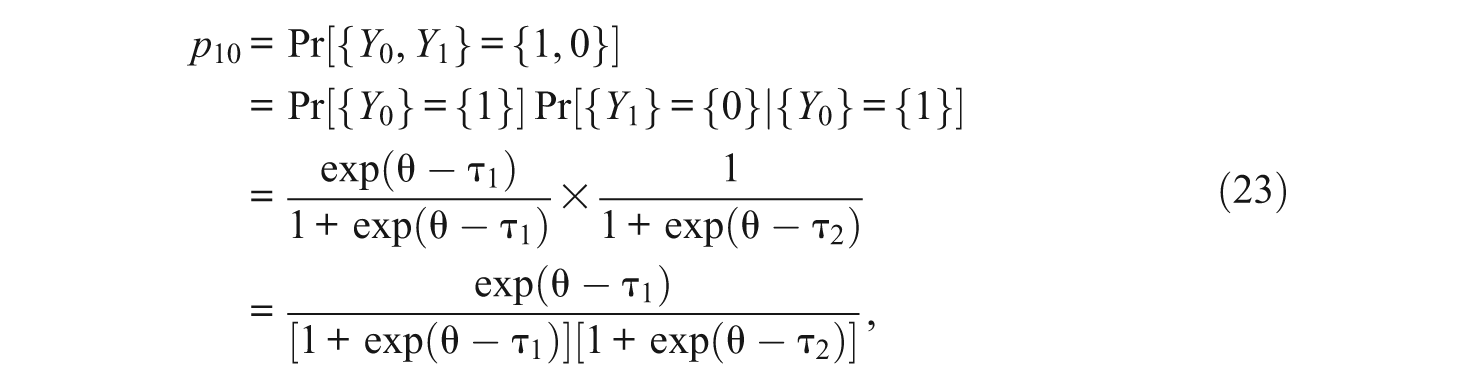
To develop the Rasch rating model, Andrich argues that there is a requirement at the level of the item for the categories to be ordered. The latent response processes must therefore be dependent so that an outcome of being successful on the second latent process and failing the first latent process cannot occur. His definition of order, therefore, is that a (latent) threshold cannot be passed unless all prior thresholds have been passed. Andrich imposes this order requirement through what he calls a Guttman structure, which says that the observation (Y₀, Y₁) = (1, 0) cannot occur. To impose this constraint, he proposes that the sample space be reduced to {(0, 0), (1,0), (1,1)}, and he computes the conditional probabilities

\begin{matrix} p_{00} = \Pr [{Y_{0}, Y_{1}} = {0, 0} | {Y_{0}, Y_{1}} = {(0, 0), (1, 0), (1, 1)}] \\ = \frac{1}{1 + \exp (θ - τ_{1}) + \exp (2 θ - τ_{1} - τ_{2})}, \end{matrix}

\begin{matrix} p_{10} = \Pr [{Y_{0}, Y_{1}} = {1, 0} | {Y_{0}, Y_{1}} = {(0, 0), (1, 0), (1, 1)}] \\ = \frac{\exp (θ - τ_{1})}{1 + \exp (θ - τ_{1}) + \exp (2 θ - τ_{1} - τ_{2})} . \end{matrix}

\begin{matrix} p_{11} = \Pr [{Y_{0}, Y_{1}} = {1, 1} | {Y_{0}, Y_{1}} = {(0, 0), (1, 0), (1, 1)}] \\ = \frac{\exp (2 θ - τ_{1} - τ_{2})}{1 + \exp (θ - τ_{1}) + \exp (2 θ - τ_{1} - τ_{2})} . \end{matrix}

It is these modeled conditional probabilities that are then used to fit the observed possible outcomes of “0” = (0, 0), “1” = (1, 0), and “2” = (1, 1).

Andrich says that the rationale for the underlying Guttman structure is that the thresholds of an item are required to be ordered.

Although instantaneously assumed to be independent, it is not possible for the latent dichotomous response processes at the thresholds to be either observable or independent—there is only one response in one of m + 1 categories. Therefore the responses must be latent. Furthermore, the categories are deemed to be ordered—thus if a response is in category x, then this response is deemed to be in a category lower than categories x + 1 or greater, and at the same time, in a category greater than categories x − 1 or lower. Therefore the responses must be dependent and a constraint must be placed on any process in which the latent responses at the thresholds are instantaneously considered independent. This constraint ensures taking account of the substantial dependence. The Guttman structure provides this constraint. (Andrich, 2005, p. 316)

While this statement seems eminently reasonable it raises two questions. Does this statement, and the derivation that corresponds to it, impose an order requirement on the values of the tau parameters? Does the statement clarify what the latent processes are? What Andrich repeatedly states but neither proves nor logically defends is that an ordering of the tau parameters is related to category ordering or is imposed through the Guttman structure.

While Andrich states that

the rationale for the Guttman structure, as with the ordering of items in terms of their difficulty, is that the thresholds of an item are required to be ordered, that is;

$τ_{1} < τ_{2} < τ_{3} < \dots < τ_{m - 1} < τ_{m}$ (Andrich, 2005, p. 313)

and then later

In the original derivation, the thresholds were made to conform to the natural order as a mechanism for imposing the Guttman structure. . . . This Guttman structure in turn implies an ordering of the thresholds. (Andrich, 2005, p. 323)

he demonstrates nothing in the move from the model defined by (8) to (11) to the model defined by (12) to (14) that requires the ordering of the tau parameters, nor connects the ordering of the tau values to the ordering of the categories.

So what are the implications of this derivation for the meaning of the tau parameters?

It appears from Figure 3 that Andrich sees the tau parameters as thresholds in the sense of Thurstone (1928). Furthermore, he says that “ $τ_{k}, k = 1, 2, 3, \dots, m$ are m thresholds which divide the continuum into m +1 categories” (Andrich, 2005, p. 311). Note, however, there is nothing in his derivation from which this follows nor does he formalize this property for use in his derivation.

To reiterate, Andrich’s mathematical derivation, starting from independent dichotomous latent processes leading to the Rasch rating model through the Guttman order restriction, holds irrespective of how one attaches substantive meaning to the latent response process.

Figure 4 is one possible formalization of the way that the thresholds might divide the continuum into m +1 categories. If the error distribution in Figure 4 were the logistic distribution, then the model that follows would not be a Rasch model. It would be, as we discuss later, Samejima’s (1969) graded response model. Note that this is not a formalization that Andrich proposes, a point made clear in Andrich (1978).

Figure 4.

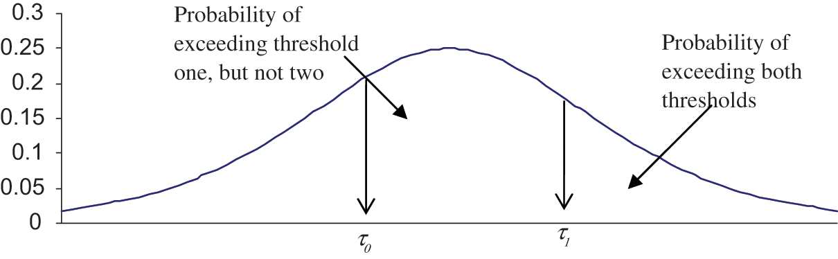
Illustration of two thresholds dividing a continuum into three parts

At the beginning of the derivation, the meanings of τ₁ and τ₂ are clear from the mathematics. τ₁ is the location on the scale where responses of 0 or 1 on the first latent process are equally likely, and similarly τ₂ is the location on the scale where responses of 0 or 1 on the second latent process are equally likely. Furthermore, these two latent processes are independent and (8) to (11) give the probabilities of observing each of the four possible events.

In a second step of the derivation, Andrich imposes the order constraint that makes the observation (Y₀, Y₁) = (0, 1) illegitimate (Andrich, 1978) and derives (12) to (14) as the conditional probabilities for (0, 0), (1, 0), and (1, 1), respectively. If τ₁ and τ₂ are considered to have their original threshold meaning, then these conditional probability expressions are simply that. They are the conditional probabilities of each of three possible outcomes on the condition that these three different outcomes are the only ones that are possible.

The meaning of τ₁ and τ₂ can be seen by noting that from (12) to (14) it follows that

\frac{p_{10}}{p_{00} + p_{10}} = \frac{\exp (θ - τ_{1})}{1 + \exp (θ - τ_{1})}

and

\frac{p_{11}}{p_{10} + p_{11}} = \frac{\exp (θ - τ_{2})}{1 + \exp (θ - τ_{2})},

which are the equivalent of (6). That is, they are parameters that describe the relationship between the probabilities of two adjacent categories conditional on the response being in one of those two adjacent categories. In other words, the instantaneous latent events, the probabilities of which are given in (7), are the events of being in the upper category given that the response is in one of two adjacent categories. The latent processes are not therefore those illustrated in Figure 3, which as we have pointed out would lead to the graded response model, not the Rasch model.

An equivalent, but informative interpretation can be illustrated if (12) to (14) are laid out in a contingency table as in Table 1.

Table 1.

The Three Probabilities in Andrich’s Derivation

	Pr(Y₁=0)	Pr(Y₁=1)
Pr(Y₂=0)	$p_{00} = \frac{1}{1 + \exp (θ - τ_{1}) + \exp (2 θ - τ_{1} - τ_{2})}$	$p_{10} = \frac{\exp (θ - τ_{1})}{1 + \exp (θ - τ_{1}) + \exp (2 θ - τ_{1} - τ_{2})}$
Pr(Y₂=1)	p₀₁=0	$p_{11} = \frac{\exp (2 θ - τ_{1} - τ_{2})}{1 + \exp (θ - τ_{1}) + \exp (2 θ - τ_{1} - τ_{2})}$

From this contingency table we immediately see that under the Rasch rating model:

\Pr (Y_{1} = 1) = \frac{\exp (θ - τ_{1}) + \exp (2 θ - τ_{1} - τ_{2})}{1 + \exp (θ - τ_{1}) + \exp (2 θ - τ_{1} - τ_{2})},

\Pr (Y_{2} = 1) = \frac{\exp (2 θ - τ_{1} - τ_{2})}{1 + \exp (θ - τ_{1}) + \exp (2 θ - τ_{1} - τ_{2})},

\begin{matrix} \Pr (Y_{1} = 1 | Y_{2} = 0) = \frac{\exp (θ - τ_{1})}{1 + \exp (θ - τ_{1})} \\ = \frac{p_{10}}{p_{00} + p_{10}}, \end{matrix}

and

\begin{matrix} \Pr (Y_{2} = 1 | Y_{1} = 1) = \frac{\exp (θ - τ_{2})}{1 + \exp (θ - τ_{2})} \\ = \frac{p_{11}}{p_{10} + p_{11}} . \end{matrix}

As shown by (17) and (18), the imposed dependence has resulted in both τ₁ and τ₂ being involved in describing the difficulties of both of the, now evidently dependent, latent processes. Furthermore, both τ₁ and τ₂ are involved in describing the difficulties of each of the three possible outcomes. The consequence is that the thresholds should not be interpreted as category difficulties as Andrich attempted to do in Figure 3. Furthermore, if the tau parameters are interpreted as thresholds of an underlying process, then that process is associated with the conditional probabilities as given in (19) and (20).

In summary, we see two misinterpretations in the language and argument that Andrich uses when deriving the Rasch rating model. First, the Guttman requirement does not impose an order requirement on the values of the tau parameters. That is, the order requirement, that (Y₀, Y₁) = (1, 0) is illegitimate, is not a requirement that τ₂ must be greater than τ₁, it just makes certain pairs of events illegitimate. Second, τ₁ and τ₂ cannot be interpreted as the difficulties of thresholds that divide up the continuum where each person is located.

These misunderstandings about the tau parameters also underpin the oft put argument that it is illogical to have disordered tau parameters. That is, it is often suggested that there is a problem if the intersection point of scores one and two is at a lower point on the scale than the intersection point of scores zero and one.

Generically, the argument is put as follows: Suppose we have a three-category item the scoring of which is as follows: “0” = fail, “1” = pass, and “2” = distinction. If data are observed for such an item and the estimated parameters are disordered, then the point on the continuum at which a student has an equal probability of a pass and distinction is at a lower level than the point on the continuum at which a student has an equal probability of being a fail or a pass. This is seen as illogical. How can it be that the point at which you are “tossing up” whether a student is a pass or a distinction is lower than the point at which you are “tossing up” whether a student is a fail or a pass?

Indeed this does sound odd, but in fact it is a misrepresentation of the situation and in particular misrepresents the meaning of the conditional probabilities involved. At the point of equal probability for pass and distinction we are not tossing up if a student should be a pass or distinction: In fact we are more confident that they are a fail (see Figure 5). Similarly at the higher level where fail and pass are equally likely, we are not tossing up if they should be assigned fail or pass, we are more confident that they are a distinction.

Figure 5.

Illustration of the relative probabilities of fail, pass, and distinction

Definitions of Order

Having questioned the connection between the ordering of the Andrich tau parameters and the ordering of the categories, it seems prudent to consider some possible formal definitions of order.

Order Definition 1

One possible definition of order is the key underpinning of the Masters derivation of the model. Suppose we consider any two response categories, c₁ and c₂, of an item. If c₂ is the higher of the two categories, then the probability of a response in category c₂ relative to the probability of a response in category c₁ must increase with the latent variable θ. This order requirement can be formalized as follows.

Definition 1

The response categories, c₁, c₂, …,c_m, of an item response model will be considered ordered if

F (j, k, θ) = \frac{\Pr (c_{k} | θ)}{\Pr (c_{j} | θ) + \Pr (c_{k} | θ)}

is an increasing function of θ for k>j.

For the Rasch rating model and using the Andersen formulation as in (2)

\begin{matrix} F (j, k, θ) = \frac{\exp (k θ_{n} - β_{ik})}{\exp (j θ_{n} - β_{ij}) + \exp (k θ_{n} - β_{ik})} \\ = \frac{\exp [(k - j) θ_{n} - (β_{ik} - β_{ij})]}{1 + \exp [(k - j) θ_{n} - (β_{ik} - β_{ij})]} . \end{matrix}

From which it follows that F(j, k, θ) satisfies Definition 1 because

\frac{dF (j, k, θ)}{d θ} = (k - j) F (j, k, θ) [1 - F (j, k, θ)] > 0,

whenever k>j, since 0<F(j, k, θ)<1.

That is, the categories of the Rasch rating model are ordered, at least by this definition, regardless of the values of the Andersen item parameters. Similarly one can show that the categories are ordered, with respect to this definition, regardless of the values of the parameters for the Masters and Andrich formulations.

Order Definition 2

A second possible definition is one that requires that the expected score on an item be an increasing function of θ. In simple terms, if one respondent has a higher value of θ than another respondent, then, on average, the respondent with the higher θ will score more.

Definition 2

Suppose the scoring function for the categories of item i are given by φ_ck = k, then the response categories, c₁, c₂ …c_m of an item response model will be considered ordered if E(X_ni|θ) is an increasing function of θ.

For the Rasch rating model and using the Andersen formulation as in (2)

$E (X_{ni} | θ) = \sum_{k = 0}^{m} k P (X_{ni} = k) .$

From which it follows that E(X_ni|θ) satisfies Definition 2 because

$\frac{dE (X_{ni} | θ)}{d θ} = \sum_{k = 0}^{m} k^{2} P (X_{ni} = k) - {[\sum_{k = 0}^{m} k P (X_{ni} = k)]}^{2} = var (X_{ni} | θ) > 0$

for all θ and regardless of the values of the item parameters.

So, as for Definition 1, the categories of the Rasch rating model are ordered, according to Definition 2, regardless of the values of the item parameters.

Parameter Estimation for the Rasch Rating Model

In the second section, we argued that in the derivation of the Rasch rating model there is no necessary connection between the ordering of the tau parameters and ordering of the categories. Then in the third section we proposed two explicit definitions of order and showed that according to these definitions the categories of the Rasch rating model are ordered regardless of the values of the tau parameters. In this section, we review the estimation of the tau parameters and in doing so note two things. First, if the estimated parameters are ordered it does not necessarily follow that the categories are ordered according to the order definitions given in the third. Second, for any given set of abilities the relative frequency of the number of responses in each category of an item is the only determinant of whether the estimated parameters are ordered or not.

Let us consider the use of maximum likelihood estimation applied to a set of L three-category items and a sample of N students for whom ability values are known. Using the Andrich formulation, as in (3), we have, for n = 1, . . ., N and i = 1, . . ., L

$P (X_{ni} = k_{ni}) = \frac{1}{γ_{ni}} \exp (\sum_{t = 0}^{k_{ni}} τ_{it} + k_{ni} (θ_{n} - δ_{i})),$

where τ_i0 ≡ 0. Note that for simplicity of the presentation we ignore the additional required constraint that $\sum_{t = 0}^{m} τ_{it} = 0$ .

As the person parameters are known we can consider the likelihood for the parameters, δ_i, τ_i1, and τ_i2 of a single item.

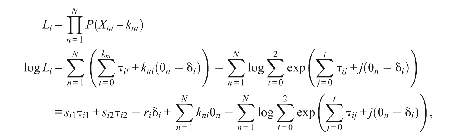
$\begin{matrix} L_{i} = Π_{n = 1}^{N} P (X_{ni} = k_{ni}) \\ \log L_{i} = \sum_{n = 1}^{N} (\sum_{t = 0}^{k_{ni}} τ_{it} + k_{ni} (θ_{n} - δ_{i})) - \sum_{n = 1}^{N} \log \sum_{t = 0}^{2} \exp (\sum_{j = 0}^{t} τ_{ij} + j (θ_{n} - δ_{i})) \\ = s_{i 1} τ_{i 1} + s_{i 2} τ_{i 2} - r_{i} δ_{i} + \sum_{n = 1}^{N} k_{ni} θ_{n} - \sum_{n = 1}^{N} \log \sum_{t = 0}^{2} \exp (\sum_{j = 0}^{t} τ_{ij} + j (θ_{n} - δ_{i})), \end{matrix}$

where s_i1 is the number of responses in Category “1” or higher on item i, s_i2 is the number of responses in Category “2” on item i, and r_i is the total score of all students on item i. The likelihood equations for the three parameters are then

$\frac{\partial \log L}{\partial δ_{i}} = - r_{i} + \sum_{n = 1}^{N} \sum_{t = 0}^{2} tP (X_{ni} = t) = 0,$

$\frac{\partial \log L}{\partial τ_{i 1}} = s_{i 1} - [\sum_{n = 1}^{N} P (X_{ni} = 1) + \sum_{n = 1}^{N} P (X_{ni} = 2)] = 0,$

and

$\frac{\partial \log L}{\partial τ_{i 2}} = s_{i 2} - \sum_{n = 1}^{N} P (X_{ni} = 2) = 0 .$

These likelihood equations make it clear that the item raw score r_i is the sufficient statistic for the item difficulty parameter δ_i, the count of students in Category “1” or higher, s_i1, is the sufficient statistic for τ_i1, and the count of students in Category “2,”s_i2, is the sufficient statistic for τ_i2. The implication of this is as follows. For a given set of students, the parameter estimates for and δ_i, τ_i1, and τ_i2 depend solely on the number of observations in each category; they are completely independent of the abilities of the students who respond in each category. This means that the ordering of the estimated values of the parameters is not connected to the abilities of the students who responded in the categories. In particular, the ordering of the mean abilities for students in each category will not influence the ordering of the item parameter estimates, which are determined solely by the numbers of students in each category.

We provide an example to illustrate the case where there is a disorder in the estimate parameters, but the item still fits the partial credit model. The item set in this example is the TIMSS 2003 released mathematics item set (TIMSS, 2003). There are 99 items in all. The student responses are from the United States data set. A partial credit model is used to fit the item responses. Six of the items are partial credit items with scores 0, 1, and 2. The remaining items are all dichotomous. All six partial credit items in this data set have disordered thresholds. As an example, we only show the results for item M032764. The item and the scoring guides are shown in Figure 6. The item statistics are shown in Figure 7. The item characteristic curves and the expected scores curve are shown in Figure 8 and Figure 9, respectively.

Figure 6.
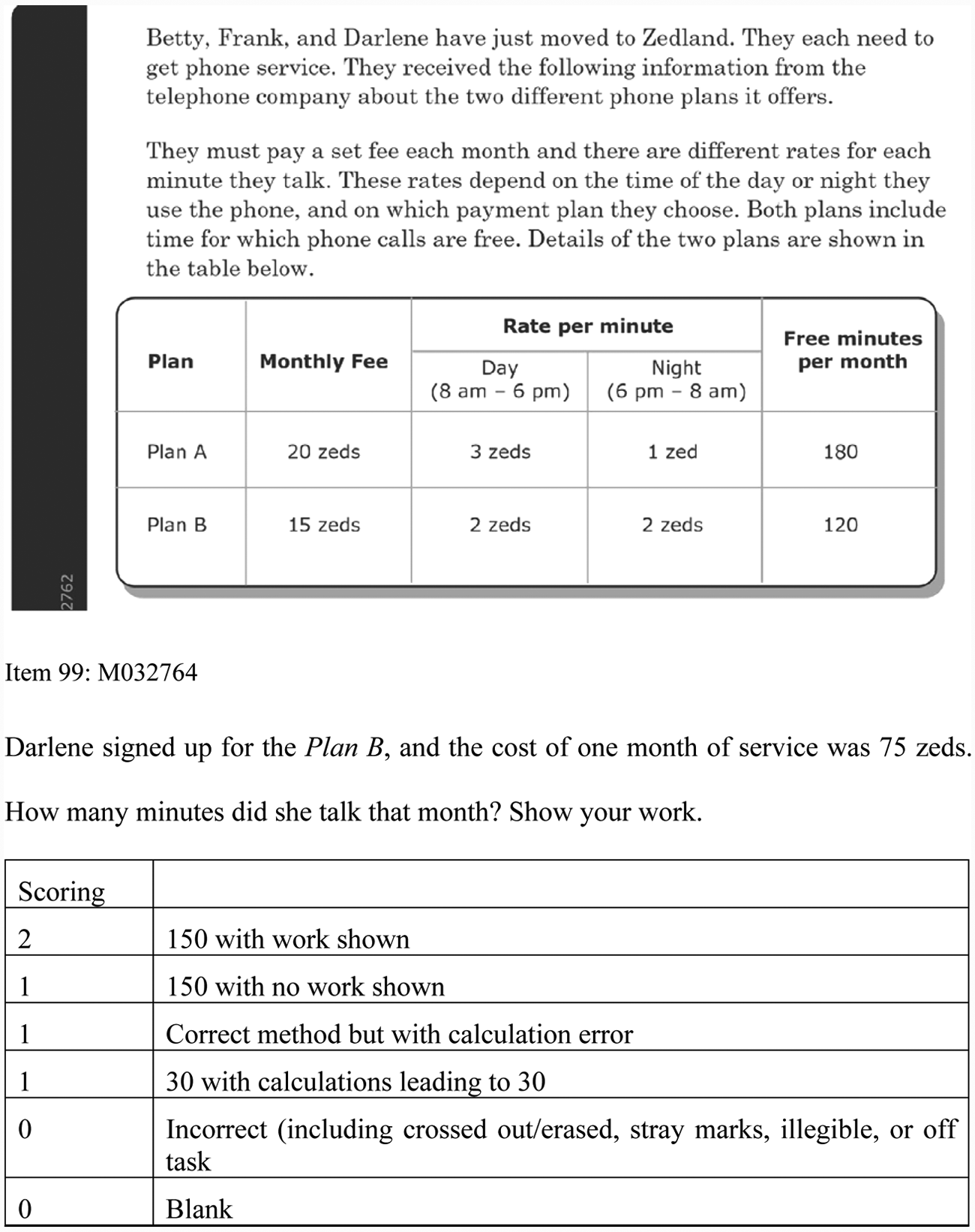
TIMSS 2003 released mathematics item (M032764)

Figure 7.
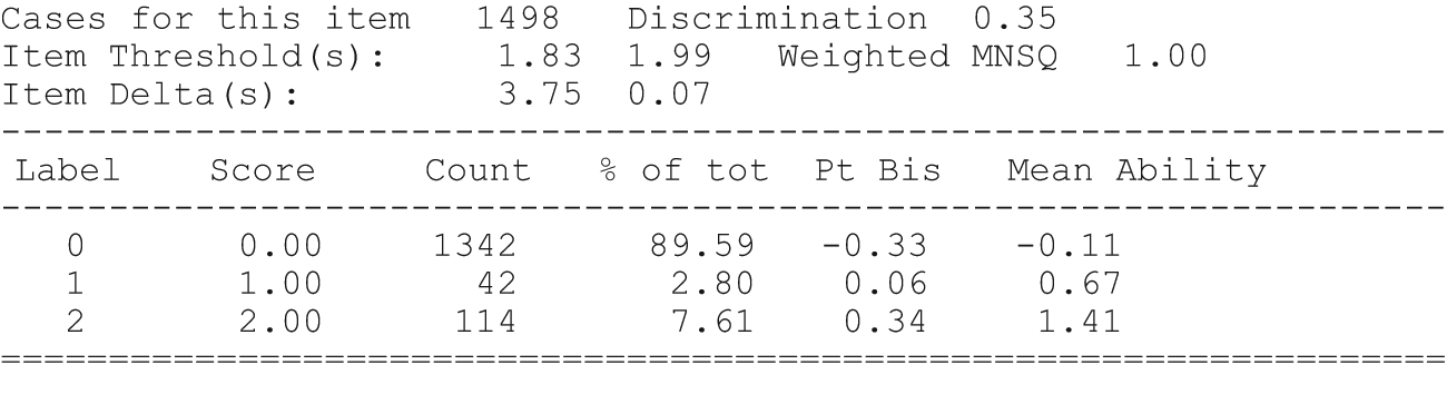
Item statistics for Item M032764

Figure 8.
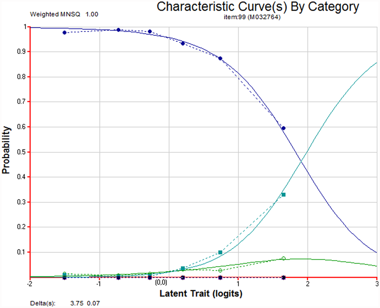
Item characteristic curves for Item M032764

Figure 9.
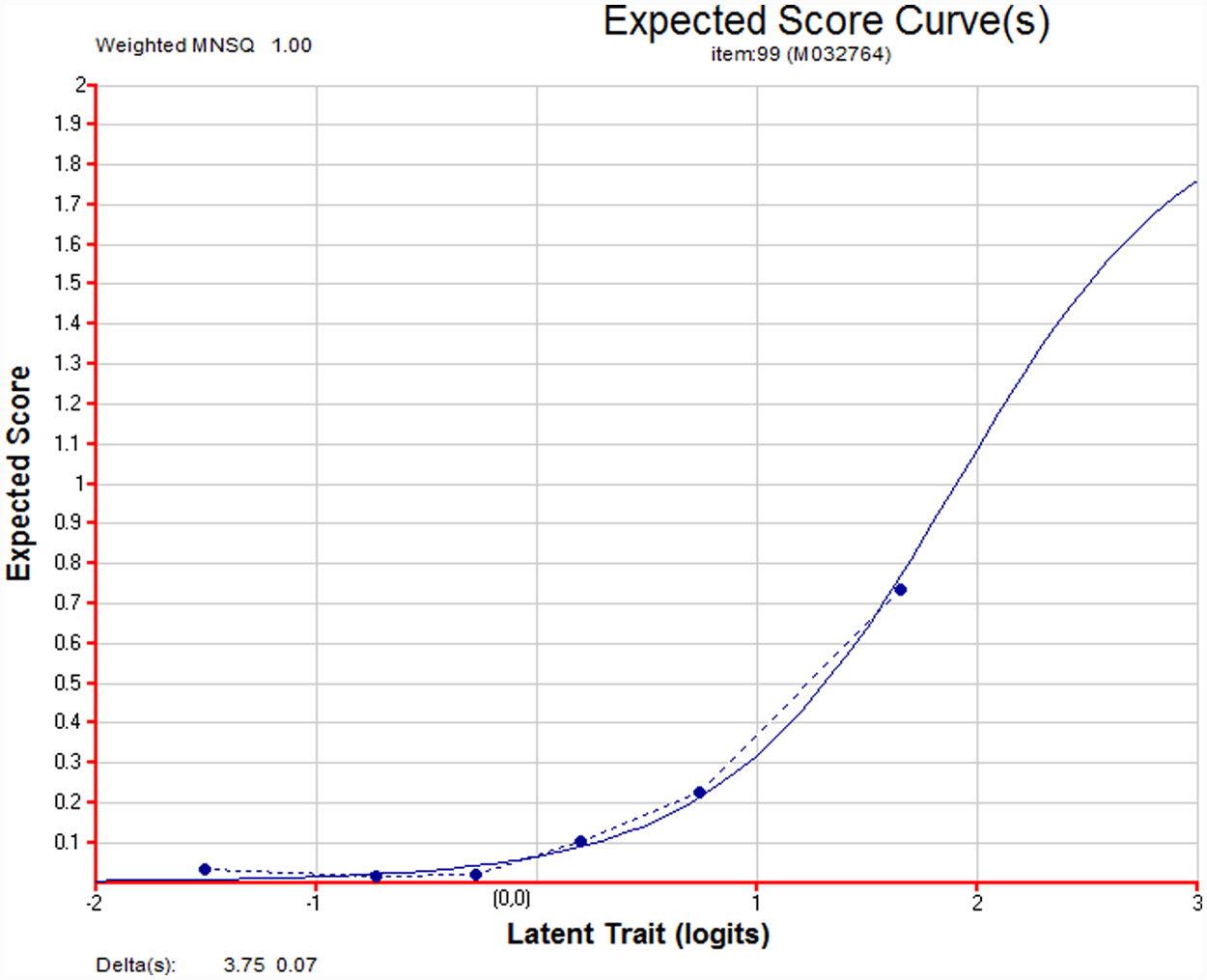
Expected scores curve for Item M032764

The item statistics shown in Figure 7 indicate that this item is difficult for the students, with 89% of the students obtaining a 0 score. Only 3% obtained a score of 1, and 8% obtained a score of 2. The item characteristic curves in Figure 8 show a low curve for score Category 1, reflecting the low frequency of responses for this score category and resulting in disordered thresholds (3.75 and 0.07).

Despite the disordered thresholds, we first note that the item weighted fit statistic is 1.00, indicating the item fit the item response model. This is further confirmed by the expected scores curve in Figure 9, showing that the observed curve and the expected curve have similar slopes and are close to each other. We also note that the observed score increases when the ability increases. This satisfies our second definition of order as described in the third section. The item statistics in Figure 7 show that the average ability of students obtaining score 1 is higher than the average ability of students obtaining score 0. Similarly, the average ability of students obtaining score 2 is higher than the average ability of students obtaining score 1. The point–biserial correlations for score Categories 0, 1, and 2 are also increasing, reflecting increasing students’ abilities across scores 0, 1, and 2. The fact that very few students obtained the middle score category leads to the disordered thresholds in numerical values, but the item still functions well in terms of model fit and in exhibiting all expected characteristics a partial credit item.

Alternative Models

To amplify further the discussion of thresholds, two alternative item response models are derived for three-category data. In each of these models the threshold parameters are well defined (at least in a mathematical sense) and their behavior can be discussed in relation to the parameters of the Rasch rating model. What we shall see at the end of this section is that even when order of the categories is clearly built into the models, the equivalent of the Rasch rating model tau parameters will in many cases be disordered.

A Sequential Model

Under the sequential model (Molenaar, 1983) for three response categories we again hypothesize two latent dichotomous items with response probabilities governed by (7), but we explicitly make the outcome of the second latent item dependent on the first. In particular, if the event Y₁ = (0) occurs, then the probability Pr(Y₂ = 1) = 0. Under this assumption a model for three response categories can be derived as follows:

$\begin{matrix} p_{00} = \Pr [{Y_{0}, Y_{1}} = {0, 0}] \\ = \Pr [{Y_{0}} = {0}] \Pr [{Y_{1}} = {0} | {Y_{0}} = {0}] \\ = \frac{1}{1 + \exp (θ - τ_{1})} \times 1 \\ = \frac{1 + \exp (θ - τ_{2})}{[1 + \exp (θ - τ_{1})] [1 + \exp (θ - τ_{2})]}, \end{matrix}$

$\begin{matrix} p_{10} = \Pr [{Y_{0}, Y_{1}} = {1, 0}] \\ = \Pr [{Y_{0}} = {1}] \Pr [{Y_{1}} = {0} | {Y_{0}} = {1}] \\ = \frac{\exp (θ - τ_{1})}{1 + \exp (θ - τ_{1})} \times \frac{1}{1 + \exp (θ - τ_{2})} \\ = \frac{\exp (θ - τ_{1})}{[1 + \exp (θ - τ_{1})] [1 + \exp (θ - τ_{2})]}, \end{matrix}$

$\begin{matrix} p_{01} = \Pr [{Y_{0}, Y_{1}} = {0, 1}] \\ = \Pr [{Y_{0}} = {0}] \Pr [{Y_{1}} = {1} | {Y_{0}} = {0}] \\ = \frac{1}{1 + \exp (θ - τ_{1})} \times 0 \\ = 0, \end{matrix}$

$\begin{matrix} p_{11} = \Pr [{Y_{0}, Y_{1}} = {1, 1}] \\ = \Pr [{Y_{0}} = {1}] \Pr [{Y_{1}} = {1} | {Y_{0}} = {1}] \\ = \frac{\exp (θ - τ_{1})}{1 + \exp (θ - τ_{1})} \times \frac{\exp (θ - τ_{2})}{1 + \exp (θ - τ_{2})} \\ = \frac{\exp (2 θ - τ_{1} - τ_{2})}{[1 + \exp (θ - τ_{1})] [1 + \exp (θ - τ_{2})]} . \end{matrix}$

Under this model the parameters τ₁ and τ₂ are the thresholds for the two latent events with an explicit dependency imposed between the two latent responses. For a complete discussion of this model, see Verhelst, Glas, and De Vries (1997). Note that while this model uses the simple logistic model at the level of the latent process, the combined model for the single three-category item is not a Rasch model in the sense of Fischer (1995).

A Cumulative Logit Model (Graded Response Model)

Under the cumulative logit model (Agresti, 1990) for three response categories, a single response mechanism is assumed, but this response process has two thresholds, τ₁ and τ₂. A latent response above τ₂ yields a “2” response, a latent response between τ₁ and τ₂ yields a “1” response, and a latent response below τ₁ yields a “0” response. This response process is illustrated in Figure 10. The distribution shown in Figure 10 is the logistic distribution.

Figure 10.
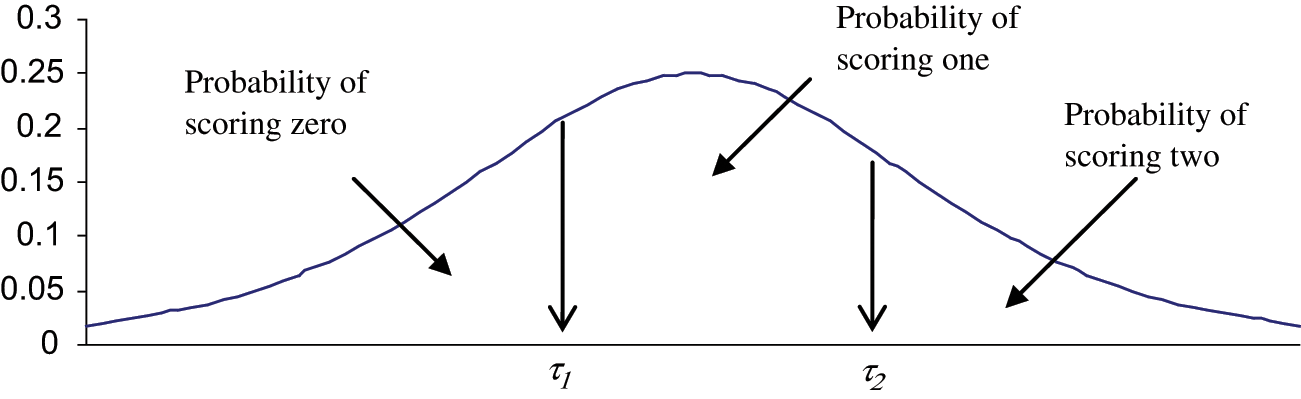
Illustration of a cumulative logit model

This model is the same model as the graded response model of Samejima (1969) and is the model that is most commonly used as the measurement model in structural equation models that permit ordinal responses to items; for example, it is standard in MPlus (Muthén & Muthén, 2006).

Under this model the probabilities for three response categories are as follows:

$p_{0} = \frac{1}{1 + \exp (θ - τ_{1})} = \frac{1 + \exp (θ - τ_{2})}{[1 + \exp (θ - τ_{1})] [1 + \exp (θ - τ_{2})]},$

$\begin{matrix} p_{1} = \frac{1}{1 + \exp (θ - τ_{2})} - \frac{1}{1 + \exp (θ - τ_{1})} \\ = \frac{\exp (θ - τ_{1}) - \exp (θ - τ_{2})}{[1 + \exp (θ - τ_{1})] [1 + \exp (θ - τ_{2})]}, \end{matrix}$

$\begin{matrix} p_{2} = \frac{\exp (θ - τ_{2})}{1 + \exp (θ - τ_{2})} \\ = \frac{\exp (θ - τ_{2}) + \exp (2 θ - τ_{1} - τ_{2})}{[1 + \exp (θ - τ_{1})] [1 + \exp (θ - τ_{2})]}, \end{matrix}$

and the parameters τ₁ and τ₂ are explicitly defined as the boundaries between the response categories. In the general case there would be m thresholds that would divide the continuum into m + 1 categories. Note that the construction of the probabilities is such that τ₁ and τ₂ can never be disordered. If they were, expression (27) would result in a negative probability.

Ordered Partition

We have already introduced the ordered partition model of Wilson (1992); it was given by (8) to (11). This model is applicable when there are multiple categories of response but the same score is applied to two or more of the categories. In the form given by (8) to (11), τ₁ and τ₂ are the difficulties of two independent items—for which, of course, there is no order requirement or expectation.

Graphical Display for the Four Models

In Figure 11, the response probabilities of each of the outcomes for each of the four models we have discussed so far are plotted for the case where τ₁ = −0.5 and τ₂ =0.5 (i.e., the taus are ordered). Recall that under the sequential model these two parameters describe the difficulty of the first and second items, respectively, and an attempt at the second item is not permitted if the first item is failed. Clearly, in each of these cases the categories are ordered.

Figure 11.
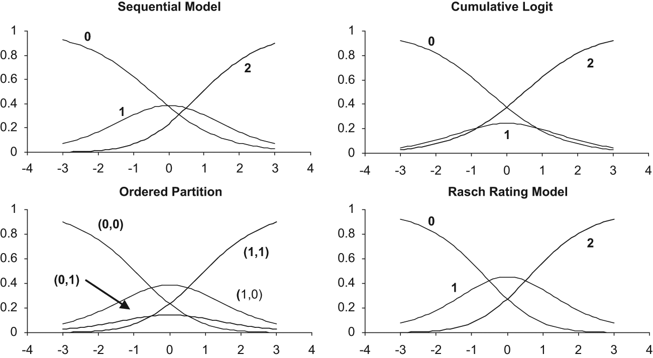
Response probabilities for the four models

For the sequential model and the ordered partition model the two parameters are the difficulties of the two items. For the cumulative model the two parameters are cut points on an underlying continuum. For the Rasch rating model the parameters describe the intersection points of “0” and “1” and “1” and “2,” respectively.

Each of the graphs in Figure 11 was constructed with the same ordered pair of parameters. Note, however, that the cumulative logit model, even with ordered thresholds on the underlying continuum, results in a “1” category that is never most probable, and the intersection point of “1” and “2” is below the intersection point of “0” and “1.” If this data pattern were modeled with the Rasch rating model, then parameter estimates would be disordered and the ordering of the categories would be refuted. That is, under the cumulative model where the categories are ordered by construction, it is possible for the intersection point of “1” and “2” to be below the intersection point of “0” and “1.”

In fact, under the cumulative model the intersection points will be reversed whenever the difference between the thresholds (the actual category boundaries) is less than approximately 1.4 logits.

The sequential model too will produce a pattern of reversed intersection points whenever the difference between the item difficulties is less than about 0.6 logits. So that even if the tau parameters are ordered and the Guttman process is required (i.e., (Y₀, Y₁) = (0, 1) is illegitimate), reversed intersection points can occur under the sequential model.

Modeling Sets of Items With the Rasch Rating Model

A number of authors (Hunyh, 1994, 1996; Verhelst & Verstralen, 1997) have explored the application of the Rasch rating model to sum scores for sets of items that conform to the simple logistic model. Their work has shown that if individual items conform to the simple logistic model, then a Rasch rating model will hold for the sum scores. Furthermore, under these circumstances the threshold parameters for the Rasch rating model must be ordered. The interesting consequence of this is that if a Rasch rating model is applied to a set of sum scores and the parameter estimates are not ordered, then the individual items cannot be modeled with a simple logistic model that assumes item (local) independence. Verhelst and Verstralen (1997), in particular, show that when modeling sum scores the Rasch rating model permits a wide variety of dependencies among the underlying items. Furthermore, exploration of this issue would seem to be a fruitful path to follow in terms of testing for item dependency with the Rasch model.

Here, we illustrate the findings of the work of Hunyh and Verhelst and Verstralen for the very simple case of two dichotomous items.

If we have two independent items, Y₁ and Y₂, that conform to the simple logistic model with item difficulty parameters α₁ and α₂, then the probabilities of the sum scores are as follows:

$\Pr (Y_{1} + Y_{2} = 0) = \frac{1}{[1 + \exp (θ - α_{1})] [1 + \exp (θ - α_{2})]},$

$\Pr (Y_{1} + Y_{2} = 1) = \frac{\exp (θ - α_{1}) + \exp (θ - α_{2})}{[1 + \exp (θ - α_{1})] [1 + \exp (θ - α_{2})]},$

and

$\Pr (Y_{1} + Y_{2} = 2) = \frac{\exp (2 θ - α_{1} - α_{2})}{[1 + \exp (θ - α_{1})] [1 + \exp (θ - α_{2})]} .$

Applying the Rasch rating model to the sum scores, the probabilities of the sum scores are, using the Masters parameterization, as follows:

$\Pr (Y_{1} + Y_{2} = 0) = \frac{1}{1 + \exp (θ - δ_{1}) + \exp (2 θ - δ_{1} - δ_{2})},$

$\Pr (Y_{1} + Y_{2} = 1) = \frac{\exp (θ - δ_{1})}{1 + \exp (θ - δ_{1}) + \exp (2 θ - δ_{1} - δ_{2})},$

and

$\Pr (Y_{1} + Y_{2} = 2) = \frac{\exp (2 θ - δ_{1} - δ_{2})}{1 + \exp (θ - δ_{1}) + \exp (2 θ - δ_{1} - δ_{2})} .$

The Rasch rating model ((32) to (34)) is equivalent to the simple logistic model ((29) to (31)) since the following functional relationships between the parameters can be established:

$e^{- α_{1}} = e^{- δ_{1}} + e^{- δ_{2}} and e^{- α_{2}} = \frac{e^{- δ_{1}} e^{- δ_{2}}}{e^{- δ_{1}} + e^{- δ_{2}}}$

$e^{- δ_{1}} = e^{- α_{1}} + e^{- α_{1}} and e^{- δ_{2}} = \frac{e^{- α_{1}} e^{- α_{1}}}{e^{- α_{1}} + e^{- α_{1}}} .$

Having established this relationship, it is also possible to show that if the Rasch rating model is applied to sum scores on items that conform to the simple logistic model, then the parameters of the Rasch rating model must be ordered. In this simple case a proof using reductio ad-absurdum is as follows.

If δ₁>δ₂, then

$\begin{matrix} - δ_{1} < - δ_{2} \\ \Rightarrow \exp (- δ_{1}) < \exp (- δ_{2}) \\ \Rightarrow \exp (- α_{1}) + \exp (- α_{2}) < \frac{\exp (- α_{1}) \exp (- α_{2})}{\exp (- α_{1}) + \exp (- α_{2})} \\ \Rightarrow {(\exp (- α_{1}) + \exp (- α_{2}))}^{2} < \exp (- α_{1}) \exp (- α_{2}) \\ \Rightarrow \exp (- 2 α_{1}) + 2 \exp (- α_{1}) \exp (- α_{2}) + \exp (- 2 α_{2}) < \exp (- α_{1}) \exp (- α_{2}) \\ \Rightarrow \exp (- 2 α_{1}) + \exp (- α_{1}) \exp (- α_{2}) + \exp (- 2 α_{2}) < 0, \end{matrix}$

which cannot be true, so we conclude that if the two sets of equations (29) to (31) and (32) to (34) are equivalent for all values of theta, then it must be the case that δ₁ ≤ δ₂

Discussion

We have argued that the ordering of the Rasch rating model thresholds is not connected to the ordering of the item response categories and that they cannot be interpreted as thresholds on an underlying continuum. In making this observation we do not dismiss the possibility that disordered estimated parameters may well be an indicator of a problem with an item. First, our discussion above, for example, has shown that if the Rasch rating model is applied to sum scores, then estimated parameter disorder is an indicator of dependence among the underlying items. Second, Andrich has shown that variations in the discrimination between adjacent categories can result in disordered estimated parameters. Third, disordered parameter estimates are indicative of low frequencies in a response category. There are a number of reasons why this may be an issue of concern, and whenever it occurs, it should be carefully reviewed by scale constructors.

While we have shown that the Andrich derivation does not depend on the nature of the latent processes and fails to demonstrate that the Guttman requirement for the latent processes imposes a numerical ordering on the tau parameters, we do not dismiss the observation that if certain psychological processes are assumed, then a numerical ordering of the tau parameters would be a substantive requirement.

If we accept the scenario of judges making independent dichotomous judgments, as illustrated in Figure 3, and then bringing them together and only accepting patterns that confirm to the Guttman requirement, then the tau parameters are estimates of the thresholds displayed in Figure 3 and disorder is a concern. The problems are, however, that we do not know the process that judges have used to produce their ratings, the model’s derivation is silent on the nature of the process, and the meaning of the parameters as thresholds requires unverifiable assumptions concerning the nature of the latent processes. The only thing that can be verified is that the tau parameters describe the events given by (15) and (16), the events of being in the upper category given that the response is in one of two adjacent categories.

What we are concerned about, however, is proliferation of the view that disordered parameters are indicative of a set of items that are not working because the categories are not ordered. As we have argued above, this is not the case; parameter disorder does not imply category disorder, unless a particular latent process is assumed; a process that can only hold when judges are involved in some judgment processes and even then the process is merely conjecture.

In perhaps the majority of applications of the Rasch rating model, no judges are involved. For example, an item may have four possible (exact) answers that are deemed appropriate to be scored as “0,”“1,”“2,” and “3,” respectively. In this case, the stochastic nature of the response resides with the student, and not with any judges, as the judgments are completely objective (because the possible answers are unambiguous). It is difficult to conceive this situation in terms of students making decisions between adjacent categories when responding. A student may provide an answer without even being aware what other possible answers there may be. In this case, under the model, students with a particular ability will have certain probabilities of providing particular answers.

The occasionally observed practice of categories being recoded to change the order on the basis of disordered parameter estimates is of particular concern as is the practice of routinely collapsing categories if the parameter estimates are not ordered (Zhu 2002; Zhu, Updyke, & Lewandowski, 2001). All these practices, when carried out solely on the basis of disordered thresholds, should be avoided.

Furthermore, we also note that the review of parameter disorder often takes place without due consideration being given to the standard errors of the parameter estimates and the covariance between them. If parameter order is of interest, then an appropriate asymptotic test of disorder, for a pair of threshold estimates, would take the form

$d = \frac{{\hat{τ}}_{2} - {\hat{τ}}_{1}}{\sqrt{var ({\hat{τ}}_{1}) + var ({\hat{τ}}_{2}) + 2 cov ({\hat{τ}}_{1}, {\hat{τ}}_{2})}},$

where d was asymptotically distributed as a standard normal deviate. Adams (1989) has shown that the covariance term in (37) can be quite large relative to the other terms in the denominator and should not be ignored.

As a final point we acknowledge that it is important to recognize that disordered parameter estimates may well be an indicator of an item that is not functioning as intended. It may, for example, indicate that some middle categories are not useful because very few respondents are using them. Furthermore, it may well indicate issues with the discrimination of the item; recall that the Rasch rating model requires equal discrimination for each of the latent processes. Items with disordered parameter estimates need to be reviewed with regard to these issues.

Footnotes

Declaration of Conflicting Interests

The author(s) declared no potential conflicts of interest with respect to the research, authorship, and/or publication of this article.

Funding

The author(s) received no financial support for the research, authorship, and/or publication of this article.

Notes

References

Adams

R. J.

(1989). Estimating measurement error (Unpublished doctoral dissertation). University of Chicago.

Agresti

(1990). Categorical data analysis. New York, NY: John Wiley.

Andersen

E. B.

(1973). Conditional inference for multiple choice questionnaires. British Journal of Mathematical and Statistical Psychology, 26, 31-44.

Andersen

E. B.

(1977). Sufficient statistics and latent trait models. Psychometrika, 42, 69-78.

Andrich

(1978). A rating formulation for ordered response categories. Psychometrika, 43, 561-573.

Andrich

(2005). The Rasch model explained. In Alagumalai

Durtis

D. D.

Hungi

(Eds.), Applied Rasch measurement: A book of exemplars (pp. 308-328). Berlin, Germany: Springer-Kluwer.

Andrich

Sheridan

Luo

(2003). RUMM2020: A Windows program for the Rasch unidimensional measurement model. Perth, Australia: RUMM Laboratory.

Fischer

G. H.

(1995). The derivation of polytomous Rasch models. In Fischer

G. H.

Molenaar

I. W.

(Eds.), Rasch models: Foundations, recent developments and applications (pp. 292-305). New York, NY: Springer Verlag.

Hunyh

(1994). On equivalence between a partial credit items and a set of independent Rasch binary items. Psychometrika, 59, 111-119.

10.

Hunyh

(1996). Decomposition of Rasch partial credit item into independent binary and indecomposable trinary items. Psychometrika, 61, 31-39.

11.

Linacre

J. M.

(1991). Step disordering and Thurstone thresholds. Rasch Measurement Transactions, 5, 171.

12.

Masters

G. N.

(1980). A Rasch model for rating scales (Unpublished doctoral dissertation). University of Chicago.

13.

Masters

G. N.

(1982). A Rasch model for partial credit scoring. Psychometrika, 47, 149-174.

14.

Molenaar

I. W.

(1983). Item steps (Heymans Bulletin HB-83-630-EX). Groningen, Germany: University of Groningen.

15.

Muthén

L. K.

Muthén

B. O.

(2006). Mplus user’s guide [Computer software and manual] (4th ed.). Los Angeles, CA: Muthén & Muthén.

16.

Nijsten

Sampogna

Chren

Abeni

(2006). Testing and reducing Skindex-29 using Rasch analysis: Skindex-17. Journal of Investigative Dermatology, 126, 1244-1250.

17.

Nilsson

A. L.

Sunnerhagen

K. S.

Grimby

(2007). Scoring alternatives for FIM in neurological disorders applying Rasch analysis. Acta Neurologica Scandinavica, 111, 264-273.

18.

Rasch

(1961). On general laws and the meaning of measurement models in psychology. In Proceedings of the IV Berkeley Symposium on Mathematical Statistics and Probability (pp. 321-333). Berkeley: University of California Press.

19.

Samejima

(1969). Estimation of latent ability using a response pattern of graded scores. Psychometrika Monographs, 34(Suppl. 17), 386-415.

20.

Thurstone

L. L.

(1928). Attitudes can be measured. American Journal of Sociology, 33, 529-554.

21.

TIMSS. (2003). TIMSS 2003 Released items. Retrieved from http://timss.bc.edu/timss2003i/released.html

22.

Verhelst

N. D.

Glas

C. A. W.

De Vries

H. H.

(1997). A steps model to analyze partial credit. In Van der Linden

W. J.

Hambleton

R. K.

(Eds.), Handbook of modern item response theory (pp. 123-138). New York, NY: Springer-Verlag.

23.

Verhelst

N. D.

Verstralen

H. H. F. M.

(1997). Modeling sums of binary items by the partial credit model (Measurement and Research Department Research Report 97-7). Arnhem, Netherlands: Cito.

24.

Wilson

(1992). The ordered partition model: An extension of the partial credit model. Applied Psychological Measurement, 16, 309-325.

25.

Wilson

M. R.

Adams

R. J.

(1993). Marginal maximum likelihood estimation for the ordered partition model. Journal of Educational Statistics, 18, 69-90.

26.

Wilson

M. R.

Adams

R. J.

(1995). Rasch models for item bundles. Psychometrika, 60, 181-198.

27.

M. L.

Adams

R. J.

Wilson

M. R.

(1997). ConQuest: Multi-Aspect Test Software [Computer program]. Camberwell, Australia: Australian Council for Educational Research.

28.

Zhu

(2002). A confirmatory study of Rasch-based optimal categorization of a rating scale. Journal of Applied Measurement, 3, 1-15.

29.

Zhu

Timm

Ainsworth

B. A.

(2001). Rasch calibration and optimal categorization of an instrument measuring women’s exercise perseverance and barriers. Research Quarterly for Exercise and Sport, 72, 104-116.

30.

Zhu

Updyke

W. F.

Lewandowski

(1997). Post-hoc Rasch analysis of optimal categorization of an ordered-response scale. Journal of Outcome Measurement, 1, 286-304.