Orthogonalizing Through Residual Centering

Abstract

Residual centering is a useful tool for orthogonalizing variables and latent constructs, yet it is underused in the literature. The purpose of this article is to encourage residual centering’s use by highlighting instances where it can be helpful: modeling higher order latent variable interactions, removing collinearity from latent constructs, creating phantom indicators for multiple group models, and controlling for covariates prior to latent variable analysis. Residual centering is not without its limitations, however, and the authors also discuss caveats to be mindful of when implementing this technique. They discuss the perils of double orthogonalization (i.e., simultaneously orthogonalizing A relative to B and B relative to the original A), the unintended consequences of orthogonalization on model fit, the removal of a mean structure, and the effects of nonnormal data on residual centering.

Keywords

residual centering latent interaction structural equation modeling confirmatory factor analysis collinearity covariates

Residual centering is a statistical technique that eliminates the covariance between two variables, allowing each to retain its unique variability (Lance, 1988). Removing unwanted variance from all indicators of a latent construct effectively removes the unwanted variance from that construct, making residual centering a useful tool for eliminating undesired variance in the context of structural equation modeling (SEM).

Residual centering removes shared variance by subtracting the expected value of target variable Y_j (i.e., ${\hat{Y}}_{j}$ ) from the observed values of Y_j, where ${\hat{Y}}_{j}$ is conditioned on a set of variables one wishes to make Y orthogonal (i.e., unrelated) to. Residual centering is therefore closely related to the more common mean centering, which subtracts ${\hat{Y}}_{j}$ from all observed values of Y_j, where ${\hat{Y}}_{j}$ is not conditioned on additional variables (i.e., ${\hat{Y}}_{j}$ = ${\bar{Y}}_{j}$ ). The only difference between residual centering and mean centering is therefore whether ${\hat{Y}}_{j}$ is conditioned on other variables.

Because mean centering does not condition ${\hat{Y}}_{j}$ on additional variables, it does not truly remove collinearity from items (i.e., mean centering does not alter variances or covariances). Mean centering instead shifts the qualitative meaning of parameter estimates (even in the case of interactions; see Echambadi & Hess, 2007). Residual centering on the other hand rotates Y_j in factor space, making it completely orthogonal to all predictors in the regression equation. Residual centering therefore does alter item variances and covariances.

Residual centering effectively removes unwanted collinearity between items and facilitates a number of statistical applications. A previous article by Little, Bovaird, and Widaman (2006) argued for using Lance’s (1988) approach when examining powered and product terms in the framework of SEM, but their article focused specifically on modeling two-way interactions (and vicariously squared latent constructs; the interaction between X and itself is the same as X²). We discuss extended applications of residual centering and present important caveats to consider when residual centering is used. We discuss four applications of residual centering in the context of SEM, including three-way interactions, exogenously controlling for covariates, accounting for collinear predictors or outcomes, and creating phantom indicators. We then discuss important caveats that researchers should consider when applying residual centering.

Method of Residual Centering

As described by Little et al. (2006), residual centering is a two-stage process by which a researcher removes unwanted variability from items or indicators before performing a target analysis. The target analysis can either examine residual-centered manifest variables or it can examine residual-centered latent constructs created by residual centering all indictors of one construct relative to all indicators of another construct.

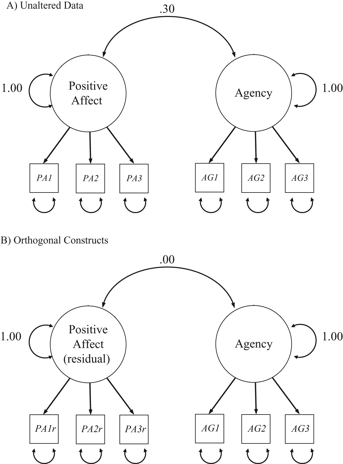
Residual centering is easily implemented with general linear model–capable software as target items are simply regressed onto items a researcher wishes to make the target variables orthogonal to. The residuals from these regressions are saved and analyzed. Online Appendix A (see online supplement at epm.sagepub.com/supplemental) presents an example of how this can be done for latent constructs. The example uses unpublished data collected by Little (1999), in which a construct of Positive Affect is made orthogonal to a construct representing Personal Agency. All indicators of Positive Affect (PA1, PA2, and PA3) are regressed onto all indicators of Personal Agency (AG1, AG2, and AG3), with the residuals saved as PA1r, PA2r, and PA3r, respectively. The residuals are then used as indicators of a residual-centered positive affect construct in a confirmatory factor analysis. Whereas the two constructs show a moderate positive correlation when the data are unaltered (see Figure 1A), Positive Affect is completely orthogonal to (i.e., uncorrelated with) Agency after residual centering (see Figure 1B).

Figure 1.

The effects of residual centering

Extended Applications

Higher Order Interactions

The basic process of residual centering is useful for removing collinearity when analyzing latent two-way interactions (Little et al., 2006) and can be easily extended to create higher order interaction constructs or higher order product terms. For instance, a construct representing the joint interaction of X, Y, and Z can be created by taking all indicators of the three constructs (e.g., X₁, X₂, X₃, Y₁, Y₂, Y₃, Z₁, Z₂, and Z₃) and creating all possible indicator-level three-way interactions (e.g., X₁Y₁Z₁, X₁Y₁Z₂, X₁Y₂Z₁, etc.). If each construct has three indicators, this process leads to 3 × 3 × 3 = 27 indicators of a latent three-way interaction.¹ Each indicator of the latent interaction will be somewhat collinear with indicators of the lower order main effects and two-way interactions, however, and it is advisable to eliminate this collinearity before testing the interaction in a structural model. Collinearity can be easily removed by residual centering indicators of the three-way interaction relative to all main effect and lower order interaction indicators.

Residual centering imposes orthogonality between an interaction term and its lower order components, only retaining random error and the nonlinear information unique to lower order indicators. Indicators of the latent interaction derived from at least one common main effect indicator will accordingly share unique variance. To account for this, latent interaction models that model all possible indicators of a latent interaction must include a number of correlated residuals to account for possible shared variance. Residual covariances must be estimated between all indicators derived from at least one common main effect indicator. As Marsh et al. (2007) have noted, this requirement can make modeling residual-centered latent interactions somewhat burdensome.

The complete orthogonality offered by residual centering makes it preferable to mean centering when examining higher order interactions. When mean centering, a higher order interaction can only be interpreted in the context of its lower order components. Mean centering therefore requires that researchers simultaneously model all lower order main effects and interactions when examining any higher order interaction. As the order of interaction increases beyond two, the number of lower order interaction indicators and constructs can make structural models unwieldy, potentially hampering model convergence.

Residual-centered indictors are inherently orthogonal to all main effect and lower order interaction indicators, however. Residual-centered higher order interactions can therefore be modeled in the absence of lower order terms without risking interpretability of its significance. It is therefore possible to test the significance of a three-way interaction without simultaneously modeling its component two-way interactions and main effects.

The close relationship between residual centering and hierarchical regression also allows researchers to determine the percentage of an outcome’s variance explained by a latent interaction without comparing models that alternatively include or omit the latent interaction term. A residual-centered interaction term is necessarily orthogonal to its constituent main effects and lower order interactions, meaning the shared variance between the residual-centered interaction and an outcome variable is necessarily unrelated to all lower order components of the interaction. Lower order components are accordingly “controlled for” through residual centering. The R² value obtained when only a residual-centered interaction term predictors Y is therefore equivalent to the change in R² between a model when only lower order components are included and a model with both the lower order components and the interaction included as predictors.

Simulation

We performed a small data simulation based on the work of Schoemann (2012) to investigate potential bias when testing three-way interactions with residual centering. This simulation compares three possible approaches to modeling latent three-way interactions: residual centering, double mean centering (e.g., Lin, Wen, Marsh, & Lin, 2010), and the latent moderated structural (LMS) equation approach (e.g., Klein & Moosbrugger, 2000). For our simulation, we generated 1,000 data sets with 1,000 observations each using Mplus, with data for the interaction generated using the LMS technique² (see Appendix B in the online supplement for data generation syntax). The generating model contained a single latent outcome variable (Y), three latent predictors (X, Z, W), all latent two-way interactions, and the latent three-way interaction. The population values for the effects of all predictors on Y were set by the equation:

Y = . 1 X + . 1 W + . 1 Z + . 1 XW + . 1 XZ + . 1 W_{1} + . 2 XWZ,

and all predictors were correlated at .30.

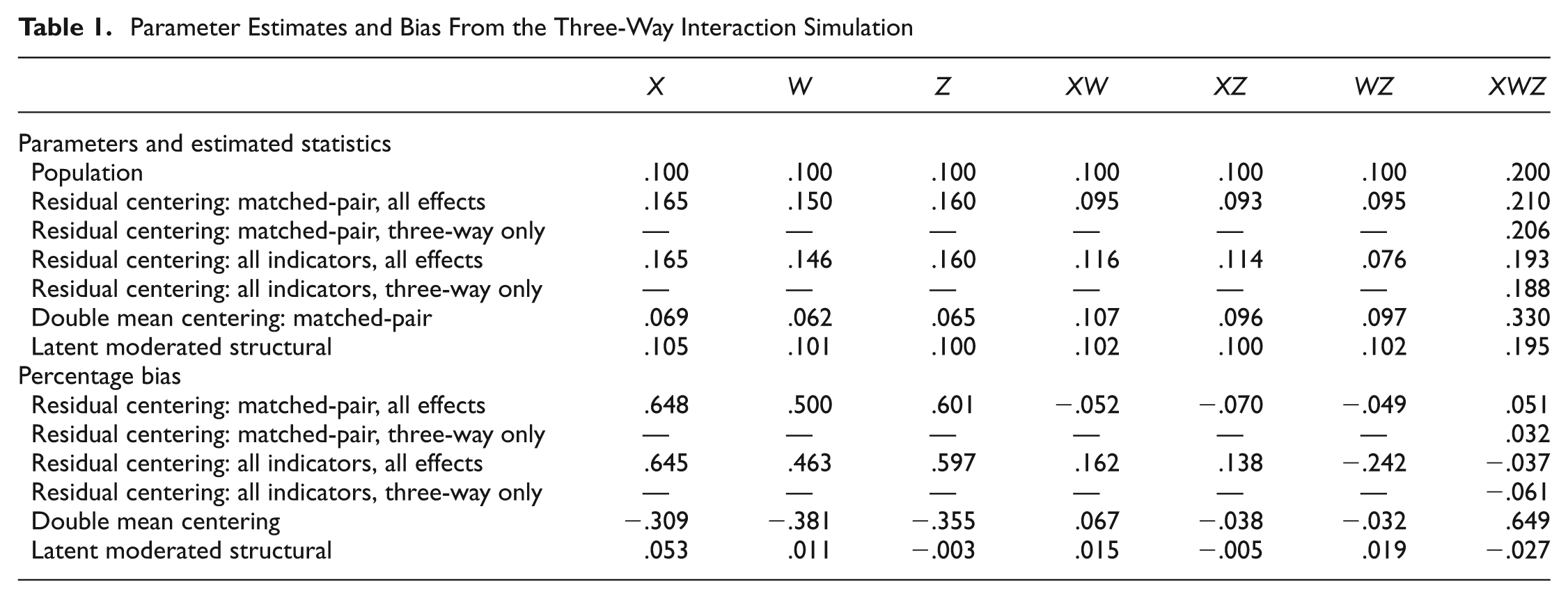
We then ran six models on each data set: (a) a residual-centered model with 3 matched-pair indicators of the three-way interaction (i.e., X₁W₁Z₁, X₂W₂Z₂, X₃W₃Z₃; see Marsh et al., 2007, for discussion of the matched-pair strategy) and all lower order main effects and interactions, (b) a residual-centered matched-pair model that contained no lower order effects, (c) a residual-centered model with all possible indictors for the three-way interaction (i.e., 27 indicators) and all possible lower order effects, (d) a similar model with 27 indicators of the latent interactions but no lower order effects, (e) a double mean-centered model (Lin et al., 2010) that included all lower order effects, and (f) an LMS model that included all possible lower order effects. We estimated all models using robust maximum likelihood to account for nonnormality of the latent interaction term. Results are presented in Tables 1, 2, and 3.

Table 1.

Parameter Estimates and Bias From the Three-Way Interaction Simulation

	X	W	Z	XW	XZ	WZ	XWZ
Parameters and estimated statistics
Population	.100	.100	.100	.100	.100	.100	.200
Residual centering: matched-pair, all effects	.165	.150	.160	.095	.093	.095	.210
Residual centering: matched-pair, three-way only	—	—	—	—	—	—	.206
Residual centering: all indicators, all effects	.165	.146	.160	.116	.114	.076	.193
Residual centering: all indicators, three-way only	—	—	—	—	—	—	.188
Double mean centering: matched-pair	.069	.062	.065	.107	.096	.097	.330
Latent moderated structural	.105	.101	.100	.102	.100	.102	.195
Percentage bias
Residual centering: matched-pair, all effects	.648	.500	.601	−.052	−.070	−.049	.051
Residual centering: matched-pair, three-way only	—	—	—	—	—	—	.032
Residual centering: all indicators, all effects	.645	.463	.597	.162	.138	−.242	−.037
Residual centering: all indicators, three-way only	—	—	—	—	—	—	−.061
Double mean centering	−.309	−.381	−.355	.067	−.038	−.032	.649
Latent moderated structural	.053	.011	−.003	.015	−.005	.019	−.027

Table 2.

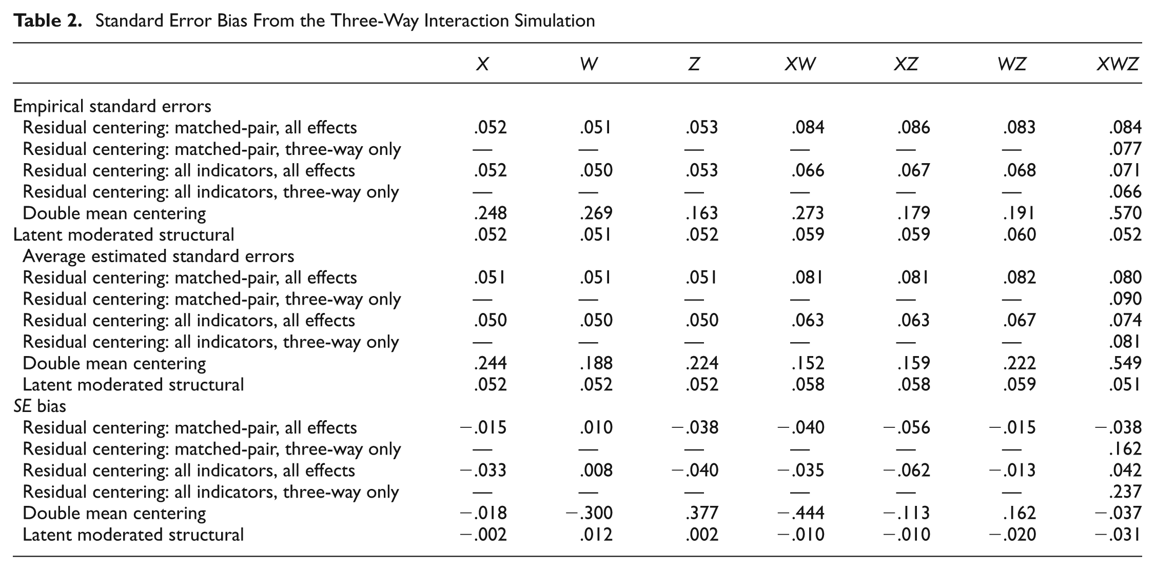
Standard Error Bias From the Three-Way Interaction Simulation

	X	W	Z	XW	XZ	WZ	XWZ
Empirical standard errors
Residual centering: matched-pair, all effects	.052	.051	.053	.084	.086	.083	.084
Residual centering: matched-pair, three-way only	—	—	—	—	—	—	.077
Residual centering: all indicators, all effects	.052	.050	.053	.066	.067	.068	.071
Residual centering: all indicators, three-way only	—	—	—	—	—	—	.066
Double mean centering	.248	.269	.163	.273	.179	.191	.570
Latent moderated structural	.052	.051	.052	.059	.059	.060	.052
Average estimated standard errors
Residual centering: matched-pair, all effects	.051	.051	.051	.081	.081	.082	.080
Residual centering: matched-pair, three-way only	—	—	—	—	—	—	.090
Residual centering: all indicators, all effects	.050	.050	.050	.063	.063	.067	.074
Residual centering: all indicators, three-way only	—	—	—	—	—	—	.081
Double mean centering	.244	.188	.224	.152	.159	.222	.549
Latent moderated structural	.052	.052	.052	.058	.058	.059	.051
SE bias
Residual centering: matched-pair, all effects	−.015	.010	−.038	−.040	−.056	−.015	−.038
Residual centering: matched-pair, three-way only	—	—	—	—	—	—	.162
Residual centering: all indicators, all effects	−.033	.008	−.040	−.035	−.062	−.013	.042
Residual centering: all indicators, three-way only	—	—	—	—	—	—	.237
Double mean centering	−.018	−.300	.377	−.444	−.113	.162	−.037
Latent moderated structural	−.002	.012	.002	−.010	−.010	−.020	−.031

Table 3.

Power From the Three-Way Interaction Simulation

Power	X	W	Z	XW	XZ	WZ	XWZ
Residual centering: matched-pair, all effects	.898	.837	.881	.231	.228	.243	.767
Residual centering: matched-pair, three-way only	—	—	—	—	—	—	.688
Residual centering: all indicators, all effects	.901	.829	.884	.459	.444	.196	.756
Residual centering: all indicators, three-way only	—	—	—	—	—	—	.680
Double mean centering	.282	.252	.258	.139	.135	.148	.468
Latent moderated structural	.528	.500	.484	.420	.402	.423	.965

Regarding the three-way interactions, our results show very low bias for the LMS and residual-centering models (i.e., absolute bias <.10) but indicated unacceptably high bias for double mean centering. Standard errors were unbiased for all models that included lower order effects but were positively biased for both models that excluded all lower order effects. Only the LMS model displayed acceptable power in these models, with the residual-centering models displaying nearly acceptable power when lower order effects were modeled. We therefore conclude that LMS is optimal for modeling latent three-way interactions and suggest residual centering with all lower order effects when LMS estimation is unavailable. Double mean centering produced positively biased parameter estimates and low power, whereas standard errors for the residual-centered models were inflated when lower order effects were omitted from our models.

Collinear Variables

Perhaps the most obvious application of an orthogonalization technique is to remove variance in one construct that is also present in one or more other constructs. Although collinear variance between an interaction term and its lower order components is a mathematical necessity that can be anticipated and simply removed from indicators of the interaction, methods for dealing other types of collinearity are less apparent. When two constructs present collinearity strong enough to affect model convergence or severely bias parameter estimates and standard errors, the most obvious remedies are to either combine all indicators into a single construct or unceremoniously drop one construct from the model (see also Cohen, Cohen, West, & Aiken 2003). If two constructs show a .95 correlation, they essentially represent the same thing and neither of these options tends to affect model interpretation.

The issue of collinear constructs becomes stickier when dropping a construct or combining the two constructs into one is not theoretically justified. Two constructs may share 90% of their variance for theoretically valid reasons (i.e., show a correlation of .95), but the remaining 10% of each construct’s variance may remain theoretically important. For example, Bargh, Gollwitzer, Lee-Chai, Barndollar, and Trötschel (2001) have hypothesized that automized self-regulation can arise through the internalization of previously effortful actions. Automized and effortful forms of self-regulation are therefore inherently related and should show a strong positive correlation. Despite this correlation, the two forms of self-regulation represent qualitatively different constructs and separate hypotheses could be made about the unique component of each.

For example, a researcher might hypothesize that rule internalization (a form of automized self-regulation) is positively related to prosocial behavior, even after controlling for effortful self-regulation. This hypothesis would normally be tested by including both automized and effortful self-regulation as simultaneous predictors of prosocial behavior, but doing so could result in collinearity if the two forms of self-regulation are highly correlated. Under such circumstances, residual centering each form of self-regulation with respect to the other would help alleviate collinearity. The residual-centered version of automized self-regulation could then be included as a predictor of prosocial behavior, with the non-residual-centered version of effortful self-regulation included as a covariate. A separate model³ could alternatively model the residual-centered version of effortful self-regulation as a predictor of prosocial behavior, with the non-residual-centered version of automized self-regulation included as a covariate.

Simulation

We performed a small data simulation to examine the effectiveness of residual centering when accommodating collinear latent predictors and compared these results with models run that used the same data but ignored collinearity. We simulated 1,000 data sets with N = 200 in which two exogenous latent factors (X₁ and X₂) predicted a single endogenous latent factor (Y). Standardized latent regressions were set to .277 and the exogenous factors were specified to correlate at .95. Each construct was indicated by three indicators and indicator communalities were set to .70.

Three structural equation models (SEMs) were run for each iteration of the simulation, with each model regressing a single endogenous latent construct onto two exogenous latent constructs. The three models respectively analyzed (a) noncentered indicators of both X₁ and X₂, (b) residual-centered indicators of X₁ but raw indicators of X₂, and (c) raw indicators of X₁ but residual-centered indicators of X₂. We combined the results from the two residual-centered data sets (i.e., the effects of the residual-centered constructs from each model) to obtain estimates of the unique relationship between each exogenous construct and Y.

Results produced moderate absolute bias for the regression coefficients (absolute biases ≈ .15) when collinearity was ignored, with a very wide distribution of each coefficient across iterations (root mean square errors [RMSEs] ≈ 11.42) and very large standard errors (power for both coefficients = 0). Residual centering, however, produced relatively unbiased estimates of the latent regression coefficients (absolute biases <.10) and much narrower sampling distributions for each coefficient (RMSEs ≈ .015; power for each = 1.00), supporting the use of residual centering when analyzing collinear latent constructs.

Controlling for Covariates

The concept of residual centering is related to controlling for covariates, and the former can in fact replace the latter. Researchers can control for covariates at the item level with residual centering and run their structural models on the residual-centered indicators. The residual-centered indicators will contain less residual variance than their raw counterparts (i.e., variance related to the covariates will be removed), implying greater power and generally better model fit as compared with controlling for covariates at the construct level. In the following example, we compare residual centering for covariates with two alternative approaches: controlling latent variables for exogenously modeled covariates (i.e., a MIMIC [multiple indicators multiple causes] model; see Brown, 2006; Jöreskog & Goldberger, 1975) and controlling individual items for endogenously modeled covariates. We again refer to the Little (1999) data described above, examining a model in which Intrinsic Motivation and Positive Affect predict Personal Agency. We control all three constructs for gender and ethnicity (represented as dummy-coded indicators) using these three methods. Online Appendix C (in the online supplement) presents SAS and LISREL syntax for all methods.

The first approach models gender and ethnicity as dummy-coded exogenous variables in the latent model and assumes that any relationship between indicators and covariates is solely because of the relations between covariates and latent constructs. This model shows the poorest—but still excellent—fit (see Table 4). The second approach models the covariates as perfect indicators of endogenous latent constructs (i.e., with residual variances fixed to zero and latent variances fixed to one). All target indictors also freely loaded onto all covariate constructs, which is equivalent to controlling individual indicators for the covariates and allows unique relations between all covariates and indicators. Controlling for covariates at the indicator level produces better model fit but requires a large number of parameter estimates to control for the covariates (see, e.g., an information criterion in Table 4). This approach to controlling for covariates may therefore complicate convergence in larger models.

Table 4.

Comparing Three Approaches to Modeling Covariates in a Structural Model

A	χ²	df	p(χ²)	RMSEA	AIC
Control constructs	56.89	48	.18	.02 (.00, .08)	140.18
Control indicators	25.30	24	.39	.01 (.00, .04)	158.60
Residual centering	25.30	24	.39	.01 (.00, .04)	66.60

	Intrinsic motivation		Positive affect		Agency
B	Standardized β	p	Standardized β	p	R ²

Control constructs	.29	<.001	.31	<.001	.18
Control indicators	.28	<.001	.31	<.001	.17
Residual centering	.28	<.001	.31	<.001	.17

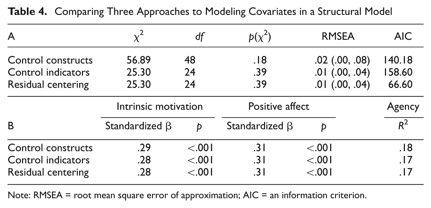
Note: RMSEA = root mean square error of approximation; AIC = an information criterion.

Our third approach controls for covariates at the item level through residual centering. We first regressed all target indicators onto all covariates and saved the residuals. The saved residuals represent the variance in each indicator, controlling for the covariates, and the residual-centered indicators were then used to represent latent constructs in a structural model.

Residual centering produced model fit and parameter estimates identical to those obtained by controlling for covariates at the indicator level within the model but required far fewer parameter estimates (see, e.g., an information criterion in Table 4). The paths controlling for the covariates are generally not of interest to researchers, and controlling for them through residual centering simply allows the implementation of a simpler structural model, which can be especially beneficial for models with many indicators.

Phantom Indicators

Residual centering is also useful when indicators are present for some—but not all—groups of a multiple group SEM. Many SEM packages require that groups have the same number of indicators (see also Widaman, Early, Grimm, Robbins, & Conger, 2009), and one way⁴ to work around this limitation is to create phantom indicators to replace indicators missing for an entire group by filling in the missing indicator(s) with randomly generated data. To ensure orthogonality of the randomly generated data, the randomly generated indicators can then be regressed on all other indicators in the model (within the group where they serve as placeholders). As before, the residuals for these regressions are saved and used as residual-centered phantom indicators. Residual-centered phantom indicators are completely orthogonal to other indicators in the model and can be easily modeled as such. Modeling residual-centered phantom indicators simply requires that their factor loadings and intercepts be fixed to zero and not be equated when testing invariance.

As Widaman et al. (2009) discuss, it is not necessary to residual-center phantom indicators; residual-centered and raw phantom indicators will produce identical results when appropriate measures are taken. As when controlling for covariates, residual centering only benefits the researcher by having fewer parameter to specify. When phantom indicators are not residual centered, residual covariances between the phantom indicators and all other indicators in the same group must be estimated for both the target and null models (see Widaman et al., 2009). Because residual-centered indicators are by definition orthogonal to all same-group indicators, implementing residual-centered phantom indicators only requires a correction to the null and target models’ degrees of freedom (df), given a properly specified null model (degrees of freedom corrections are discussed in the Caveats section below).

Example

We present an example from the Little (1999) data in which seventh and eighth graders provided self-reports of Positive and Negative Affect (syntax provided in Online Appendix D in the online supplement). Three indicators were measured for each construct in both groups, and we selectively deleted one indicator of Negative Affect in the seventh-grade sample. The deleted indicator was replaced with random normal data, which were regressed onto all other indicators in the seventh-grade data set. The residuals from this regression were stored and the originally generated random indicator was deleted from the data. The resulting data set contained six indicators, three indicating Positive Affect, two indicating Negative Affect, and one that was completely orthogonal to all other variables (i.e., a phantom indicator).

The original complete data for the eighth-grade sample and the phantom-indicated data for the seventh-grade sample were then analyzed as a two-group confirmatory factor analysis in LISREL. The eighth-grade sample was estimated using three indicators per construct and local identification was obtained using the fixed-factor approach. The latent correlation between Positive and Negative Affect was freely estimated. An identical model was run on the seventh-grade sample, except that the factor loading and intercept for the phantom indicator was fixed to zero (see Figure 2). Fit of this model was then calculated based on a properly specified null model (numerical details discussed in the Caveats section below).

Figure 2.

The phantom indicator does not load onto Negative Affect in the seventh-grade sample

Partial factorial invariance models were run to establish invariance of the parameters across the two groups, with invariance examined by both the likelihood ratio test (i.e., the change in χ²) and by examining the change in the comparative fit index (CFI; see Meade, Johnson, & Braddy, 2008). Partial invariance was specified because we anticipated a priori that parameter estimates for the phantom indicator in the seventh-grade data set would not equate with the same indicator in the eighth grade (complete) data. Weak invariance was established by equating all factor loadings, excluding that of the phantom indicator, Δχ²₍₃₎ = 8.02, p > .01; Δdf-corrected CFI = .002, and strong invariance was established by equating all intercepts across groups, excluding the intercept for the phantom indicator, Δχ²₍₃₎ = 7.62, p > .01; Δdf-corrected CFI = .001. Thus, weak and strong invariance were established across groups, despite each group having a different number of indicators.

Caveats

The Pitfall of Double Orthogonalization

We previously described how to use orthogonalized variables in order to examine the unique effect of one construct, controlling for the variance shared with another highly collinear construct. In our example, we discussed creating two data sets, one for each orthogonalized construct. This approach was necessary because residual centering two items/constructs relative to each other results in residuals that are themselves correlated with the same magnitude but opposite direction as the original items/constructs. Using both sets of residuals in a single data set would reintroduce collinearity into the model.

To demonstrate that two orthogonalized residuals are in fact correlated to the same magnitude but reversed direction as the original indicators, it is instructive to consider the variables geometrically. Each indicator can be represented as a line originating from some common point in construct space (e.g., the origin), with the angle between the two indicators’ lines (in degrees) equal to the inverse cosine of the two items’ correlation. Two completely orthogonal constructs are represented by lines separated by 90°, that is, cos⁻¹(0) = 90. Perfectly positively correlated items are separated by 0°, that is, cos⁻¹(1.00) = 0, and perfectly negatively correlated items are separated by 180°, that is, cos⁻¹(−1.00) = 180.

If we take two items, A and B, which are correlated .866, they can be represented by lines separated by 30° (Figure 3A). Orthogonalizing B with respect to A causes A to remain stationary but increases the angle between A and B′ to 90° (Figure 3B). Orthogonalizing A with respect to the original B results in the lines represented in Figure 3C, which have a 150° angle between them (30 + 30 + 90 = 150). The cosine of this angle reveals a correlation that is the exact opposite of the correlation between our two original indicators (−.866). Mathematically, this relationship can be written thus:

Figure 3.

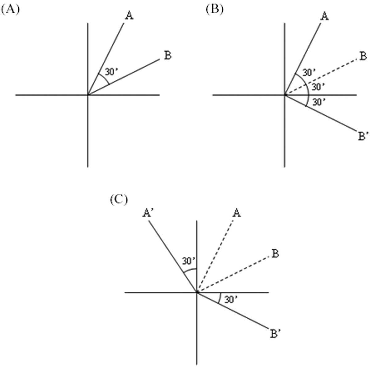
Double orthogonalization re-introduces the collinearity between two variablesNote: The original variables A and B correlate .87 when separated by a 30° angle. In (B), the variable B is made orthogonal to the original A. In (C) the variable A is made orthogonal to the original B. The orthogonalized variables of A and B are now separated 180 − 30 = 150°, resulting in a negative correlation of −.87.

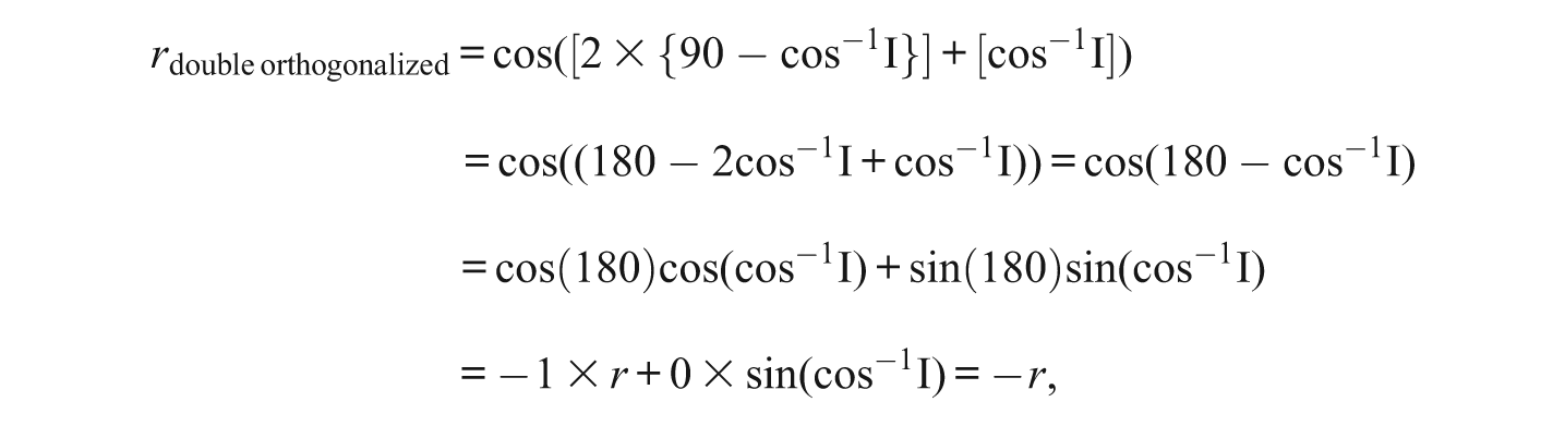
\begin{matrix} r_{double orthogonalized} = cos ([2 \times {90 - co s^{- 1} I}] + [co s^{- 1} I]) \\ = cos ((180 - 2 co s^{- 1} I + co s^{- 1} I)) = cos (180 - co s^{- 1} I) \\ = cos (180) cos (co s^{- 1} I) + sin (180) sin (co s^{- 1} I) \\ = - 1 \times r + 0 \times sin (co s^{- 1} I) = - r, \end{matrix}

where r represents the original correlation between the indicators, cos⁻¹I is the angle representing the original correlation, and 90 − cos⁻¹I represents the number of degrees one indicator must move to become orthogonal to the other.

Degrees of Freedom and Fit Indices

Residual centering biases measures of model fit because several elements of the input covariance matrix and mean vector can be perfectly fit as zeros. Because these elements are zero by definition, they are not truly free to vary and should not be counted toward the model’s overall degrees of freedom. In the phantom indicator example described earlier, the phantom indicator was made artificially orthogonal to the five true indicators in the seventh-grade group, meaning five input data elements were not truly free to vary and should not be counted toward the model’s overall degrees of freedom.

Fit indices were corrected by subtracting 5 from both the fitted and null model’s degrees of freedom and recalculating each index. Root mean square error of approximation (RMSEA), CFI, and Tucker–Lewis index were recalculated based on the corrected df values using the formulas available in Hu and Bentler (1998). In the phantom indicator example, a correctly specified null model produced a χ² of 3104.264, with results indicating 41 degrees of freedom. The estimated χ² is unbiased, but five elements of the input data were not truly free to vary. A corrected null degrees of freedom is therefore 41 − 5 = 36. Likewise, the configural invariance model produced an unbiased χ² value of 37.491 but incorrectly assumed 18 degrees of freedom. The degrees of freedom were again corrected by subtracting 5 from the model-provided degrees of freedom to account for the five input parameters that were not truly free to vary (df = 18 − 5 = 13). A corrected RMSEA was then obtained by using the observed χ² value, the corrected degrees of freedom for the configural model, and the total sample size, N = 760; $RMSEA = \sqrt{((37.491 - 13) / (760 - 1)) / 13} = . 050 .$ Similarly, corrected information from the null and configural models was used to obtain a corrected CFI (1 − (37.491 − 13)/(3104.264 − 36) = .992) and Tucker–Lewis index ((3104.264/35 − 37.491/13)/(3104.264/36 − 1) = .978).

Table 5 presents the observed and corrected fit indices for the phantom indicator example. As the table shows, correcting for the inflated degrees of freedom did not significantly affect model fit in this example. The degrees of freedom correction in this example was relatively minor, however, and more significant changes in model fit would be expected for models with more extensive residual centering. A model that includes two main effect constructs (three indicators each) and their residual-centered interaction (having 3 × 3 = 9 indicators) would contain 9 × 6 = 54 artificial degrees of freedom in the covariance matrix, which could have more serious implications for model fit.

Table 5.

Observed and Corrected Fit Indices for the Phantom Indicator Example

Configural	Observed	Corrected
RMSEA	.052	.050
CFI	.993	.992
TLI	.988	.978

Weak	Uncorrected	Corrected

CFI	.991	.990
ΔCFI	.002	.002

Strong	Uncorrected	Corrected

CFI	.989	.989
ΔCFI	.002	.001

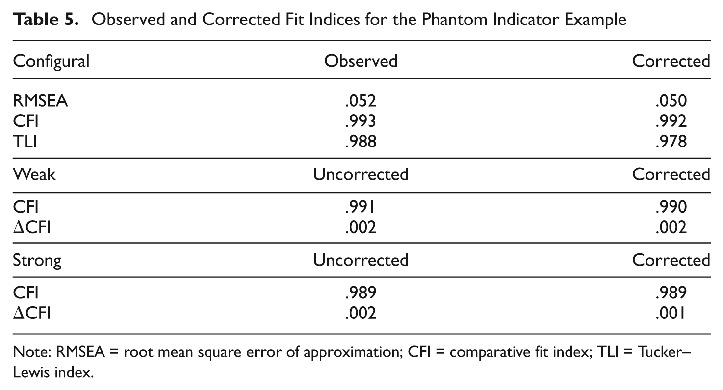
Note: RMSEA = root mean square error of approximation; CFI = comparative fit index; TLI = Tucker–Lewis index.

An alternative approach to correcting degrees of freedom was proposed by Widaman et al. (2009). In their approach, residual variances (and intercepts) artificially fixed to zero are freely estimated. This effectively corrects degrees of freedom for the estimated model. Widaman et al. (2009) showed that this method does not bias the estimated value of chi-square and that the model provides the correct degrees of freedom. This approach does not, however, correct the degrees of freedom for the null model, and relative fit indices will still be slightly biased when using their approach.

Furthermore, Widaman et al.’s (2009) approach requires that residual-centered indicators freely covary with all indicators they are orthogonal to. Their approach specifically dealt with the instance of phantom indicators (which are orthogonal to all other indicators in the model), and it is unknown how their approach will affect model fit when only specific constructs are forced to orthogonality. Estimating the residual covariance of orthogonalized indicators is not likely to bias model fit (nor should estimating other trivial residual correlations) but does lead to less parsimonious models.

Removal of a Mean Structure

The intercept of a regression equation represents the expected value of Y after controlling for all predictors, meaning all residuals obtained through residual centering necessarily have a mean of zero. This artificial removal of the mean structure will not affect the results of correlational analyses but will obviously affect tests of mean differences. When item means are substantively important, a mean structure must be reintroduced for residual-centered variables.

The mean structure is easily reintroduced for residual-centered indicators by storing the estimated intercept from each residual-centering regression equation and adding that value back to the estimated residuals. If group means are specifically of interest, residual centering with mean reintroduction can be done separately by group or by including group membership and the interaction between group membership and all predictors in the regression equation. When group membership and all interactions are included in the model, the effect of group must also be added to non–reference group’s residuals. Reintroduced residual means represent conditional means after controlling for all predictors (i.e., expected group means when all covariates are zero, which will depend on how the covariates are scaled) and can be compared with each other in the same way as group differences are examined in analysis of covariance.

Although residual centering with mean reintroduction allows for direct comparison of conditional means in a general linear model framework, analyzing these same variables as indicators of latent variables requires some additional considerations. For example, the relationship between a target variable and any predictor included in the residual-centered regression equation is not guaranteed to be equivalent across groups. The conditional mean of a residual-centered indicator may therefore have a qualitatively different meaning for each group and tests of strong invariance may not be reasonable. Because factorial invariance determines whether model parameters can be equated across groups or across time after conditioning on differences in the underlying latent construct (i.e., not conditioning on the latent construct and all covariates), factorial invariance should be tested before residual centering. Residual-centered indicators can then be additionally tested for invariance, with a lack of invariance in the residual-centered indicators but not in the uncentered indicators interpreted as arising from group differences in the residual-centering regression equations.

Example

We present an example using the Little (1999) data that consider self-report measures of aggression⁵ and frustration tolerance (e.g., “I easily get angry when things don’t go the way I want”) in eighth-grade students. Here we test the hypothesis that males show higher levels of aggression than females but that this difference is largely because of differences in frustration tolerance. To test this hypothesis, we performed latent t tests on aggression both before and after controlling for frustration tolerance through residual centering (example syntax SAS presented in Online Appendix E).

Analysis of the raw data confirmed both weak invariance, Δχ²₍₂₎ = 0.242, p > .001, ΔCFI < .001, and strong invariance, Δχ²₍₂₎ = 0.79, p > .001, ΔCFI < .001. Latent means were not equal across groups, Δχ²₍₁₎ = 57.44, p < .001, and our results confirmed that males reported higher levels of aggression (M = 1.41, SE = .02) than females (M = 1.21, SE = .01).

Analysis of the residual-centered data also supported weak invariance, Δχ²₍₂₎ = 0.20, p > .001, ΔCFI< .001, and strong invariance, Δχ²₍₂₎ = 0.99, p > .001, ΔCFI < .001. Comparison of the latent means indicated that aggression was actually lower in males (M = .80, SE = .02) than females (M = .93, SE = .01) after controlling for differences in frustration tolerance, Δχ²₍₁₎ = 41.95, p < .001.

Skew and Residual-Centered Indicators

Regression assumes normally distributed data and residuals, and residual centering does not consistently produce latent orthogonality when raw data are skewed (e.g., Lin et al., 2010). The product of latent variables score should be residual centered relative to latent variable main effects, not relative to the main effect indicators. Lin et al. found that the regression coefficients obtained using manifest indicators do not accurately estimate the regression coefficients using latent variables when main effect latent variables were not normally distributed. The product of latent variables is therefore not completely independent of latent main effects. Lin et al. found unacceptable bias when examining residual-centered two-way interactions created from moderately skewed latent main effects (e.g., skew ≈ 1.14). These results indicate that residual centering is best implemented when the normality assumption of latent main effects is reasonable.

This caveat applies especially to applications of residual centering that involve orthogonalizing latent interactions, and the assumption of normality may be especially violated when considering higher order interactions. As the product of two normally distributed variables is not normal (MacKinnon, Lockwood, & Williams, 2004), the higher order interaction will be the product of a nonnormal product variable (X₁X₂) and a normal variable (X₃). As a result, residual centering could be biased for higher order interactions. The three-way interaction simulation presented above, however, indicates that at least three-way interactions remain relatively unbiased when first-order indicators are multivariate-normally distributed. Further research is needed to determine how violations of normality in one or more indicators affect such interactions.

Discussion

Residual centering is useful for overcoming many modeling problems, such as providing researchers with a tool for removing collinearity between interaction terms and their respective main effects and for removing collinear variability from individual constructs. Residual centering also allows researchers to control for covariates outside of their structural models and allows for phantom indicators that serve as nonmeaningful placeholders in multiple group models.

Researchers interested in residual-centering their data should bear the several caveats in mind, however. The four limitations we discussed above involve the perils of double orthogonalization, the impact of orthogonalizing on model fit, the removal of a mean structure, and bias when residual centering with skewed indicators. As we have suggested, double orthogonalization can be avoided by creating multiple data sets, the bias in model fit can be removed through relatively simple corrections, and a mean structure can be easily reintroduced to residual-centered data. Similarly, researchers should be especially mindful of the normality assumption when implementing residual centering as even slightly nonnormal data may pose problems. Despite its limitations, however, residual centering is a useful addition to any data analyst’s tool kit, and we encourage its wider application in the field.

Footnotes

Acknowledgements

The authors would like to acknowledge Jie Chen for assisting with the preparation of this article.

Declaration of Conflicting Interests

The author(s) declared no potential conflicts of interest with respect to the research, authorship, and/or publication of this article.

Funding

The author(s) disclosed receipt of the following financial support for the research, authorship, and/or publication of this article: This work was supported in part by the Center for Research Methods and Data Analysis (Todd D. Little, Director) in the College of Liberal Arts and Sciences at the University of Kansas (for more information visit ) and a grant from the John Templeton Foundation.

Notes

References

Bargh

J. A.

Gollwitzer

P. M.

Lee-Chai

A. Y.

Barndollar

Trötschel

(2001). The automated will: Nonconscious activation and pursuit of behavioral goals. Journal of Personality and Social Psychology, 81, 1014-1027.

Brown

T. A.

(2006). Confirmatory factor analysis for applied research. New York, NY: Guilford.

Cohen

West

S. G.

Aiken

L. S.

(2003). Applied multiple regression/correlation analysis for the behavioral sciences (3rd ed.). Mahwah, NJ: Erlbaum.

Echambadi

Hess

J. D.

(2007). Mean-centering does not alleviate collinearity problems in mode rated multiple regression models. Marketing Science, 26, 438-445.

Bentler

P. M.

(1998) Fit indices in covariance structure modeling: Sensitivity to underparameterized model misspecification. Psychological Methods, 3, 424-453.

Jöreskog

K. G.

Goldberger

A. S.

(1975). Estimation of a model with multiple indicators and multiple causes if a single latent variable. Journal of the American Statistical Association, 70, 631-639.

Klein

Moosbrugger

(2000). Maximum likelihood estimation of latent interaction effects with the LMS method. Psychometrika, 65, 457-474.

Lance

C. E.

(1988). Residual centering, exploratory and confirmatory moderator analysis, and decomposition of effects in path models containing interactions. Applied Psychological Measurement, 12, 163-175.

Lin

Wen

Marsh

H. W.

Lin

(2010). Structural equation models of interactions: Clarification of orthogonalizing and double-mean-centering strategies. Structural Equation Modeling, 17, 374-391.

10.

Little

T. D.

(1999). Hamden study of adolescents. Unpublished raw data.

11.

Little

T. D.

Bovaird

J. A.

Widaman

K. F.

(2006). On the merits of orthogonalizing powered and product terms: Implications for modeling interactions among latent variables. Structural Equation Modeling, 13, 497-519.

12.

MacKinnon

D. P.

Lockwood

C. M.

Williams

(2004). Confidence limits for the indirect effect: Distribution of the product and resampling methods. Multivariate Behavioral Research, 39, 99-128.

13.

Marsh

H. W.

Wen

Hau

Little

T. D.

Bovaird

T. D.

Widaman

K. F.

(2007). Unconstrained structural equation models of latent interactions: Contrasting residual- and mean-centered approaches. Structural Equation Modeling, 14, 570-580.

14.

Meade

A. W.

Johnson

E. C.

Braddy

P. W.

(2008). Power and sensitivity of alternative fit indices in tests of measurement invariance. Journal of Applied Psychology, 93, 568-592.

15.

Schoemann

A. M.

(2012). Three-way interactions in structural equation modeling. Unpublished manuscript.

16.

Widaman

K. F.

Early

D. R.

Grimm

K. J.

Robbins

R. W.

Conger

R. D.

(2009). Investigating factorial invariance of latent variables across populations when manifest variables are missing completely. Manuscript submitted for publication.

Supplementary Material

Please find the following supplemental material available below.

For Open Access articles published under a Creative Commons License, all supplemental material carries the same license as the article it is associated with.

For non-Open Access articles published, all supplemental material carries a non-exclusive license, and permission requests for re-use of supplemental material or any part of supplemental material shall be sent directly to the copyright owner as specified in the copyright notice associated with the article.

0.00 MB

0.03 MB