Generalized IRT Models for Extreme Response Style

Abstract

Extreme response style (ERS) is a systematic tendency for a person to endorse extreme options (e.g., strongly disagree, strongly agree) on Likert-type or rating-scale items. In this study, we develop a new class of item response theory (IRT) models to account for ERS so that the target latent trait is free from the response style and the tendency of ERS is quantified. Parameters of these new models can be estimated with marginal maximum likelihood estimation methods or Bayesian methods. In this study, we use the freeware program WinBUGS, which implements Bayesian methods. In a series of simulations, we find that the parameters are recovered fairly well; ignoring ERS by fitting standard IRT models resulted in biased estimates, and fitting the new models to data without ERS did little harm. Two empirical examples are provided to illustrate the implications and applications of the new models.

Keywords

item response theory extreme response style random threshold Bayesian methods

Likert-type or rating-scale items are widely used in psychological inventories or questionnaires to measure personality, interest, or attitude. It is commonly observed that a respondent may consistently use only a few of the given options. In such cases, an observed response is a combination of a respondent’s attitude and response bias. The term response style indicates a systematic tendency to use a limited number of options. Research has suggested that response style is content independent and reflects different types of item functioning across respondents (Jackson & Messick, 1958; Johnson, 2003; Rorer, 1965).

Several response styles have been noted. Baumgartner and Steenkamp (2001) summarize seven important response styles: acquiescence, disacquiescence, net acquiescence, extreme response, response range, midpoint responding, and noncontingent responding. Among them, extreme response style (ERS) has attracted much research attention (Greenleaf, 1992; Hamilton, 1968; Van Vaerenbergh & Thomas, 2013; Weijters, Geuens, & Schillewaert, 2010). ERS denotes a systematic tendency to endorse extreme options. The opposite testing behavior, mild response style (MRS), denotes a systematic tendency to endorse middle options (Hurley, 1998). For example, in a 5-point agreement scale (1 = strongly disagree, 2 = slightly disagree, 3= neutral, 4 = slightly agree, 5 = strongly agree) or a 5-point satisfaction scale (1 = very dissatisfied, 2 = somewhat dissatisfied, 3 = neither satisfied nor dissatisfied, 4 = somewhat satisfied, 5 = very satisfied), Options 1 and 5 are considered as extreme options, whereas Options 2, 3, and 4 are considered mild options. Likewise, in a 4-point frequency scale (1 = never, 2 = seldom, 3 = often, 4 = always) or a 4-point performance scale (1 = poor, 2 = fair, 3 = good, 4 = excellent), Options 1 and 4 are considered extreme options, whereas Options 2 and 3 are considered mild options. These two terms are mutually exclusive (ERS and MRS cannot be observed at the same time on an item). That is, a strong tendency toward ERS means a weak tendency toward MRS, and vice versa. Thus, ERS is used throughout this study.

Hamilton (1968) reviewed a series of studies on ERS and concluded that ERS reflects respondents’ personality attributes. It is argued that respondents who frequently exhibit ERS have a motivation to achieve clarity, precision, and decisiveness in verbal statements (Johnson, Kulesa, Llc, Cho, & Shavitt, 2005); respondents who complete surveys quickly and are simplistic thinkers are most likely to exhibit ERS (Naemi, Beal, & Payne, 2009); ERS is not affected by the length of response options (Kieruj & Moors, 2010); and ERS is rather stable across time (Weijters et al., 2010). Literature has shown the relationship between ERS and individual- and society-level variables (Arce-Ferrer, 2006; Baumgartner & Steenkamp, 2001; Chen, Lee, & Stevenson, 1995; van Herk, Poortinga, & Verhallen, 2004). Because ERS causes undesired interference with the normal response process, test validity and inference are threatened (De Beuckelaer, Weijters, & Rutten, 2010). Within the framework of item response theory (IRT), it was found that ERS could contaminate the precision of latent traits targeted for measurement and could result in biased estimates of item parameters (Bolt & Newton, 2011; van Herk et al., 2004).

Outside the IRT framework, studies on ERS within the raw-score framework have been conducted in various ways. An intuitive strategy is to investigate the target latent traits and ERS using the same item responses but different scoring rubrics. For example, extreme options are counted as a measure of ERS (Johnson et al., 2005). Unfortunately, as documented in the literature, item characteristics and person measures are mutually confounded and cannot be separated within the framework of classical test theory (Embretson & Reise, 2000); thus, the measures of the target latent traits and ERS are not separable when the same item responses are used. Because the selection of items is less critical in the identification of ERS (De Beuckelaer et al., 2010), another strategy is to use heterogeneous items (in content) to investigate response styles, in which a sample of items is randomly selected from a wide range of scales such that contents and response styles are separated (Greenleaf, 1992; Weijters et al., 2010; Weijters, Schillewaert, & Geuens, 2008). For example, three items each are sampled from 10 scales. The major drawback of this strategy is that the target latent traits cannot be measured precisely with such a short test for each latent trait.

The following five issues deserve clarification. First, the identification of ERS requires a large number of items. The larger the number, the better the identification will be. For example, 16 items were used by Greenleaf (1992) for the identification of ERS. Second, the identification also requires a large number of options. Again, the larger the number the better the identification will be. For example, it is much easier to identify ERS with 7-point scales (1 = strongly disagree, 2 = disagree, 3 = somewhat disagree, 4 = neutral, 5 = somewhat agree, 6 = agree, and 7 = strongly agree) than 3-point scales (e.g., 1 = disagree, 2 = neutral, and 3 = agree). Third, there is no clear categorization for extreme responses. In the aforementioned 3-point scale, we may all agree that Options 1 and 3 are extreme responses. However, in the aforementioned 7-point scale, some may argue that Options 1 and 7 are extreme responses, whereas others may argue that Options 1, 2, 6, and 7 are extreme responses. Fourth, different categorizations of extreme responses (e.g., Options 1 and 7 vs. Options 1, 2, 6, and 7 in a 7-point scale) will lead to different results. It is thus recommended that different categorizations be adopted and the results be compared. Finally, our models should detach ERS from the target latent traits so that the “purified” latent traits are valid for comparison.

The rest of this article is organized as follows. First, we review several existing IRT models. Second, we develop a new class of IRT models to account for ERS so that the resulting measures for the latent traits are valid for comparison. Third, we outline the parameter estimation procedures and computer software for the new class of models. Fourth, we present a series of simulation studies to examine the parameter recovery of the new class of models, evaluate the consequences of ignoring ERS by applying standard IRT models, and summarize our findings. Fifth, we give two empirical examples of an interpersonal conflicts scale and a civic education survey to illustrate the implications and applications of the new models. Finally, we present our conclusions and make suggestions for future studies.

IRT Models for ERS

One advantage of IRT is that person parameters and item parameters can be separated. Many IRT models have been proposed for analyzing Likert-type or rating-scale items, such as the partial credit model (PCM; Masters, 1982), the rating scale model (RSM; Andrich, 1978), and the graded response models (Samejima, 1969). For example, the PCM and RSM can be written, respectively, as

log (\frac{P_{nij}}{P_{ni (j - 1)}}) = θ_{n} - (δ_{i} + τ_{ij})

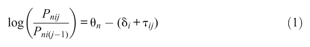
and

log (\frac{P_{nij}}{P_{ni (j - 1)}}) = θ_{n} - (δ_{i} + τ_{j}),

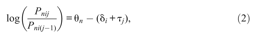
where P_nij and P_ni_{(j − 1)} are the probabilities of receiving scores j and j− 1 on item i for person n; θ_n is the latent trait of person n; δ_i is the overall difficulty of item i; τ_ij is the jth threshold parameter (relative to δ_i) for item i (in the PCM), and τ_j is the jth threshold parameter (relative to δ_i) for all items (in the RSM). In the PCM, RSM, and other standard IRT models, it is assumed that, conditional on item parameters, θ_n is the only factor that determines the item responses. When response styles also play a role in item responses, such an IRT model becomes inappropriate.

Persons with different levels of ERS could be grouped into latent classes (Moors, 2008; van Rosmalen, van Herk, & Groenen, 2010). The PCM can be extended to accommodate latent classes:

log (\frac{P_{ngij}}{P_{ngi (j - 1)}}) = θ_{ng} - (δ_{gi} + τ_{gij}),

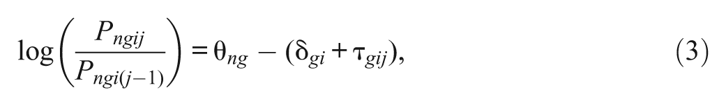
where g denotes the latent class membership. The labeling of the latent classes in the mixture PCM (Equation 3) can be determined by inspecting the threshold parameter estimates. It was frequently found that one latent class had a large distance between adjacent thresholds, whereas another latent class had only a small distance between adjacent thresholds (Rost, Carstensen, & von Davier, 1997; von Davier, Eid, & Zickar, 2007). The distance between adjacent thresholds represents the likelihood of exhibiting extreme responses; the larger the distance, the smaller the likelihood. Using the mixture PCM to investigate ERS should be done with caution because it may not always reveal true latent classes and may yield spurious latent classes (Alexeev, Templin, & Cohen, 2011).

The multidimensional nominal response model has been adopted to account for quantitative differences in ERS (Bolt & Johnson, 2009; Bolt & Newton, 2011; Johnson & Bolt, 2010). In the model, the log-odds of selecting option j over option R (the reference category) are defined as

log (\frac{P_{nij}}{P_{ni R}}) = α'_{ij} θ_{n} + β_{ij} γ_{n} + τ_{ij},

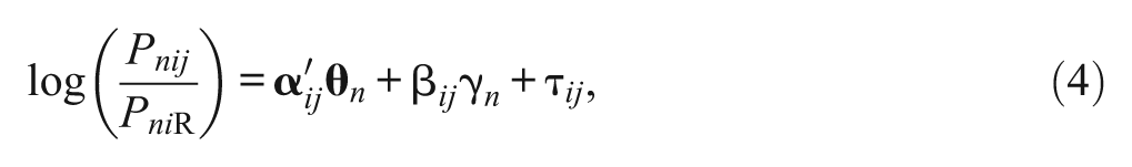
where P_nij and P_ni_R are the probabilities of selecting options j and R on item i for person n, respectively; $θ_{n}$ is the vector of the target latent traits of person n; γ_n is a latent trait of exhibiting ERS of person n; $α_{ij}$ and β_ij are the slope parameters of option j in item i on θ and γ, respectively; and τ_ij is the location parameter of option j in item i. A larger γ value indicates a stronger tendency toward ERS. This model, although it accounts for individual differences in θ and γ, ignores the ordinal nature of response options in Likert-type or rating-scale items. Furthermore, it lacks a theoretical justification as to why γ (the ERS tendency) can compensate for θ.

Items may function differently for different persons. Johnson (2003) proposes a heterogeneous thresholds probit model for ordinal responses, in which a person can have his or her own thresholds. After constructing a symmetric space of latent responses and centering the thresholds across persons, distances between adjacent thresholds are obtained. The vector of the distances is assumed to follow a multivariate log-normal distribution. A person with a larger distance between adjacent thresholds exhibits ERS more frequently. Although this model portrays individual differences in exhibiting ERS, it does not quantify the tendency of persons to exhibit ERS.

In contrast to the cumulative IRT models for ERS, Javaras and Ripley (2007) adopt unfolding IRT models (Luo, 2001) to study ERS. Following the same idea of random thresholds across persons (Johnson, 2003), Javaras and Ripley develop a multidimensional unfolding model that allows thresholds to vary across persons. Group- or individual-specific thresholds are derived from a scalar parameter on common thresholds and a translation parameter. Although this model can quantify both acquiescence and ERS, the inherited ideal-point unfolding approach is not applicable when item response functions are cumulative (i.e., the higher the level of the latent trait, the higher the probability of endorsement). In practice, many Likert-type or rating-scale items are analyzed with cumulative IRT models. It is important to develop cumulative IRT models for ERS, which is the major purpose of this study.

Another way to quantify ERS is to classify item responses into two categories—extreme responses and nonextreme responses—and then fit a standard IRT model to the reconstructed data set (de Jong, Steenkamp, Fox, & Baumgartner, 2008). For the reconstructed data set, a latent trait denoting the tendency to perform ERS is measured. Although this approach is straightforward in assessing ERS and is easy to implement, it fails to yield measures of the target latent trait.

Different persons may have different perspectives on the given options. A person may consider the threshold between strongly disagree and disagree large, whereas another person might consider it small. To account for such a random nature, a random-threshold model and its extensions (Wang, Wilson, & Shih, 2006; Wang & Wu, 2011) have been developed, in which the threshold parameters in the RSM are treated as random effects:

log (\frac{P_{nij}}{P_{ni (j - 1)}}) = θ_{n} - (δ_{i} + τ_{nj})

and

τ_{nj} ~ N (τ_{j}, σ_{j}^{2}),

where τ_nj is the jth threshold for person n and is assumed to follow a normal distribution with a mean of τ_j and variance of $σ_{j}^{2}$ . If $σ_{1}^{2} = σ_{2}^{2} = \dots = σ_{J}^{2} = 0$ (i.e., no randomness in the thresholds across persons; J is the number of thresholds), this model simplifies to the RSM. Likewise, the thresholds in the PCM (Equation 1) can be random effects:

log (\frac{P_{nij}}{P_{ni (j - 1)}}) = θ_{n} - (δ_{i} + τ_{nij})

and

τ_{nij} ~ N (τ_{j}, σ_{j}^{2}),

where τ_nij is the jth threshold of item i for person n; and the other variables have been defined previously. Although the random-threshold RSM (Equations 5 and 6) and the random-threshold PCM (Equations 7 and 8) may be used to describe response styles across persons, they do not directly quantify the tendency toward ERS.

Two conclusions can be drawn from reviewing the aforementioned models. First, treating thresholds as random effects can account for response styles. Second, it is desirable to have an index to directly quantify the amount of ERS for individual persons. To achieve these goals, a class of IRT models for ERS is developed in this study.

Formulation of the New ERS Models

To account for the tendency toward ERS across persons, we revise Equations (5) and (7) as

log (\frac{P_{nij}}{P_{ni (j - 1)}}) = θ_{n} - (δ_{i} + ω_{n} τ_{j})

and

log (\frac{P_{nij}}{P_{ni (j - 1)}}) = θ_{n} - (δ_{i} + ω_{n} τ_{ij}),

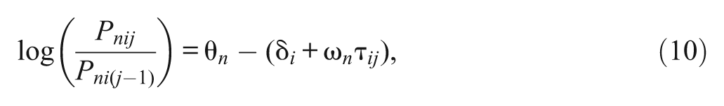
where ω_n is a weight parameter of respondent n on thresholds and is assumed to follow a log-normal distribution with a mean of zero and variance of $σ_{ω}^{2}$ ; and the others have been previously defined. The θ and ω random-effect variables are assumed to be independent because the literature has shown that the ERS tendency is quite stable across contents. A large ω indicates a large distance between thresholds, such that the extreme options are less likely to be endorsed. In addition, $σ_{ω}^{2}$ depicts the magnitude of inconsistency of experiencing item stimuli among persons: the larger the value of $σ_{ω}^{2}$ , the more heterogeneous experience in the thresholds across persons. Equation (9) is referred to as the ERS model with rating scale modeling (ERS-RSM) and Equation (10) as the ERS model with partial crediting modeling (ERS-PCM). When $σ_{ω}^{2}$ is zero (or equivalently ω = 1 for all persons), these two models simplify to the RSM and PCM, respectively.

Figure 1 exhibits the effects of different ω values on the response probabilities of a four-point item. When ω = 1, the item response functions are equivalent to those in the PCM, so they can be treated as a reference. When ω = 0.5, the shape of the item response functions becomes narrower, such that the probabilities of scoring 1 or 4 (extreme options) become larger than they are when ω = 1. On the other hand, when ω = 2, the shape of the item response functions becomes wider, such that the probabilities of scoring 1 or 4 become smaller than they are when ω = 1. When ω is increased to 5, the probability of extreme responses approaches zero. Apparently, a smaller ω value indicates a stronger tendency to exhibit ERS.

Figure 1.

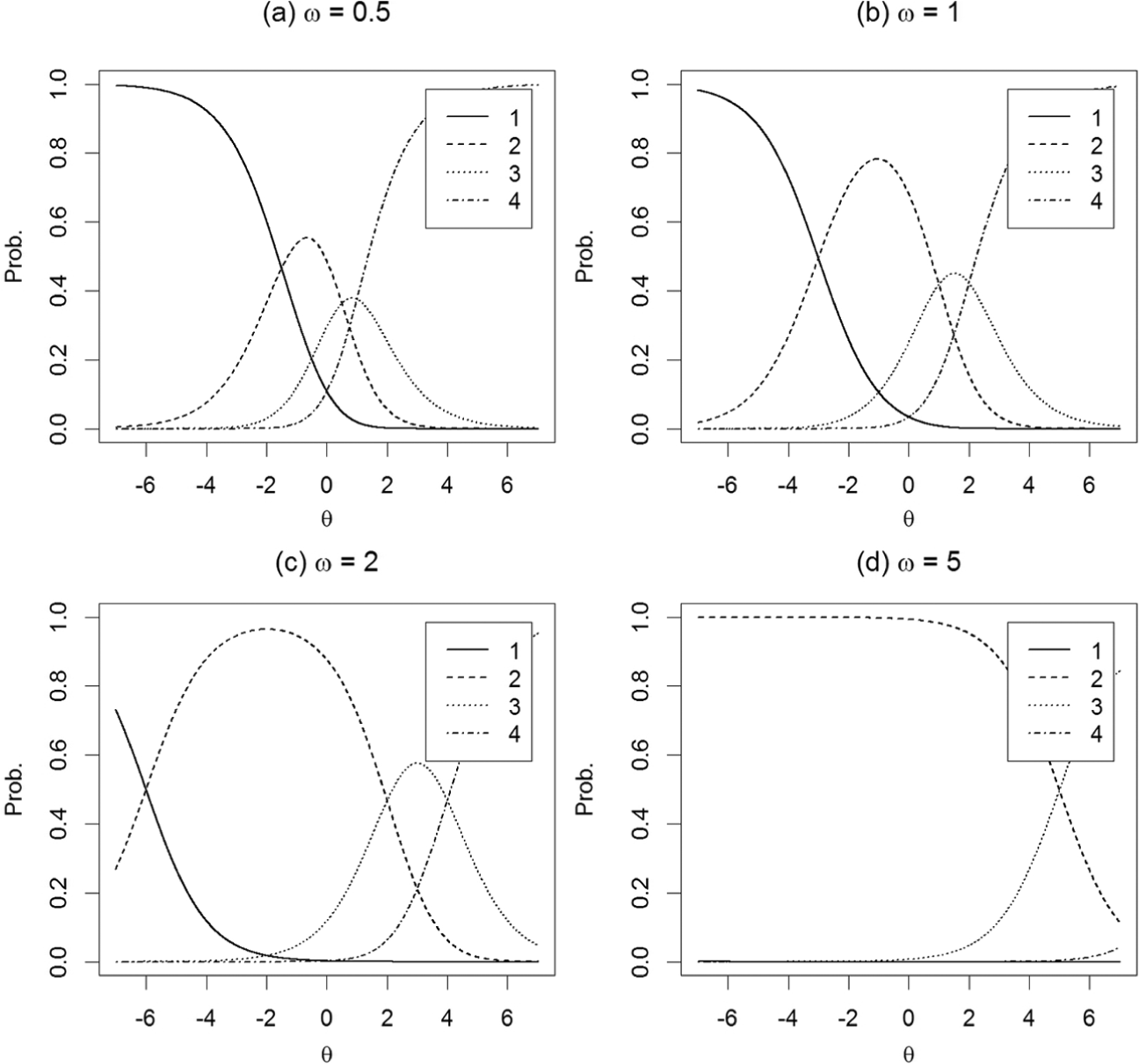
Item response functions for persons with different ω values in a hypothetical four-point item (α = 1, δ = 0, τ₁ = −3, τ₂ = 1, and τ₃ =2).

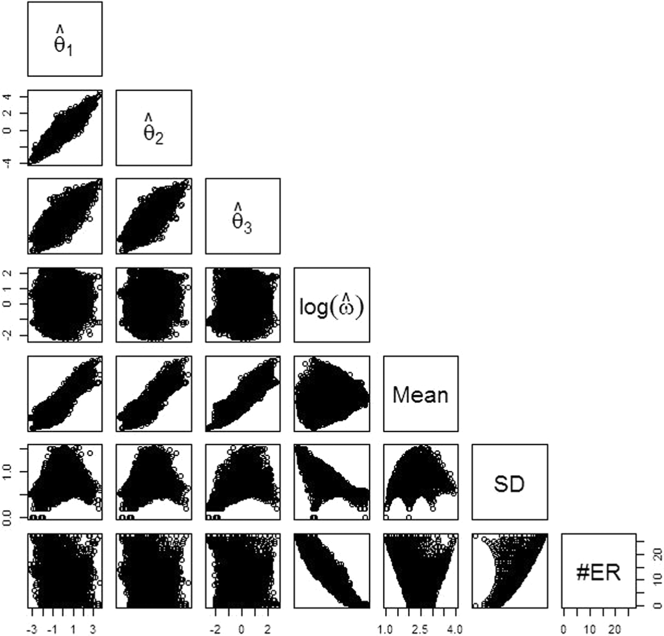
To describe the ERS-PCM, we simulated a data set of 1,000 persons and 40 six-point items following the ERS-PCM, with $σ_{ω}^{2} = 0 . 9^{2}$ . For each person, we computed the mean and SD of the item scores across the 40 items and the number of extreme responses, which was defined as the number of times in the 40 items that an endorsed option was either the lowest or highest option. Figure 2 shows the relationships among the θ, log(ω), the mean of item scores, the SD of item scores, and the number of extreme responses. It can be shown that θ is positively correlated with the mean of item scores (r = 0.97); log(ω) is negatively correlated with the SD of item scores (r = −0.61) and the number of extreme responses (r = −0.82); the SD of item scores is positively correlated with the number of extreme responses (r = 0.39); and the other correlations are very small (−0.14 < r < 0.16). In other words, the mean of the item score helps depict θ, and the SD of the item score and the number of extreme responses help depict ω.

Figure 2.

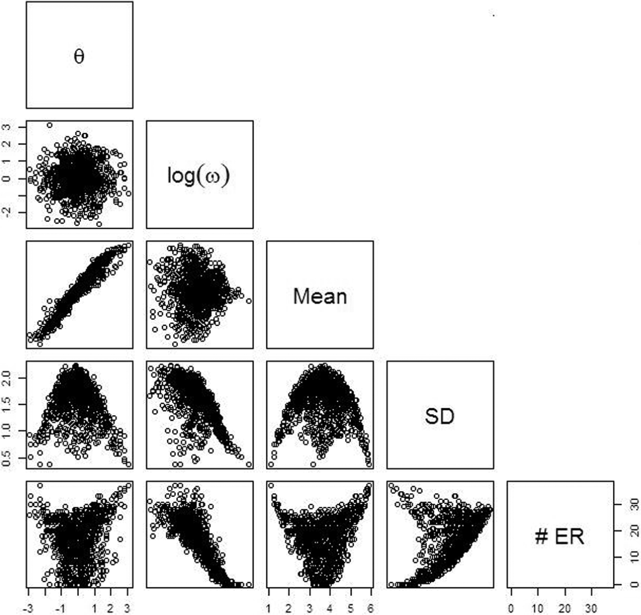
Scatter plots of the θ and log(ω) values, the mean and SD of raw item scores, and the number of extreme responses (#ER) of a simulated data set.

Although the ERS-PCM (Equation 10) shares a common feature with the random-threshold PCM (Equation 7), they have very different conceptualizations. In both models, thresholds are treated as random effects to account for the interaction between persons and items. In the random-threshold PCM, there are as many as J− 1 random effects to account for the interaction (see Equation 8), whereas in the ERS-PCM there is only one random effect, ω. The J− 1 random effects in the random-threshold PCM have to be compared with the target latent trait to describe their impacts, whereas a person’s ω value in the ERS-PCM can directly account for his or her tendency toward ERS.

Generalization of the ERS-PCM is straightforward. For example, like many IRT models, one can incorporate a slope parameter into the ERS-PCM:

log (\frac{P_{nij}}{P_{ni (j - 1)}}) = α_{i} [θ_{n} - (δ_{i} + ω_{n} τ_{ij})],

where α_i denotes the discrimination power of item i with respect to θ, and the other variables have been defined previously. Equation (11) is referred to as the ERS model with generalized partial credit modeling (ERS-GPCM). When ω_n = 1 for all persons, the model simplifies to the generalized PCM (Muraki, 1992).

In the aforementioned ERS models, the target latent trait θ is unidimensional. In practice, a person may be requested to respond to multiple scales, each measuring a latent trait (or a scale with multiple subscales, each measuring a latent trait). Although these scales can be analyzed one at a time, it has been shown that such a consecutive unidimensional approach is less statistically efficient than the multidimensional approach where all scales are analyzed jointly (Adams, Wilson, & Wang, 1997; Cheng, Wang, & Ho, 2009). To implement the multidimensional approach, Equations (10) and (11) can be extended as

log {(\frac{P_{nij}}{P_{ni (j - 1)}})}_{s} = θ_{ns} - (δ_{is} + ω_{ns} τ_{ijs})

and

log {(\frac{P_{nij}}{P_{ni (j - 1)}})}_{s} = α_{is} [θ_{ns} - (δ_{is} + ω_{ns} τ_{ijs})],

where subscript s indexes scales (s = 1, . . ., S). The θ and ω variables are assumed to be independent, but the θ_s variables can be correlated, and the ω_s variables can also be correlated. In Equations (12) and (13), each person receives a ω value on each scale to depict his or her ERS tendency on that scale. These two models can be simplified by constraining a common ω value for each person across scales:

log {(\frac{P_{nij}}{P_{ni (j - 1)}})}_{s} = θ_{ns} - (δ_{is} + ω_{n} τ_{ijs})

and

log {(\frac{P_{nij}}{P_{ni (j - 1)}})}_{s} = α_{is} [θ_{ns} - (δ_{is} + ω_{n} τ_{ijs})],

where ω_n does not have subscript s, indicating a person has a single ω value to describe their ERS tendency. This kind of constraint is also imposed in the unfolding IRT models developed by Javaras and Ripley (2007).

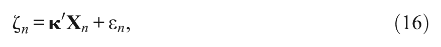
Covariates can be added to account for the variations in the random effects, which is referred to as latent regression because the criterion variables are latent rather than observed (Adams, Wilson, & Wu, 1997). Apart from θ, ω can be regressed on a set of covariates. Because ω_n follows a log-normal distribution, let ζ_n≡ log(ω_n) and X_n represent the covariates for person n. The regression is formed:

ζ_{n} = κ' X_{n} + ε_{n},

where κ is the vector of regression coefficients, and ε_n is an error term following a normal distribution with mean zero.

Parameter Estimation

The ERS-PCM and its variations (e.g., Equations 11 -16) belong to nonlinear mixed models. The parameters can be estimated by using marginal maximum likelihood estimation methods, which have been implemented in the computer program SAS NLMIXED (SAS Institute, 1999). In addition, recent years have witnessed a rapid development in Bayesian estimation with Markov chain Monte Carlo (MCMC) methods and the popularity of the freeware WinBUGS (Spiegelhalter, Thomas, Best, & Lunn, 2007) on IRT models (Curtis, 2010). In this study, we adopt WinBUGS for parameter estimation. In Bayesian estimation, a statistical model and prior distributions of model parameters are specified to yield a joint posterior distribution. Because the joint posterior distribution is often very difficult to obtain, MCMC methods thus come into play. After a sequential sampling, the posterior distribution of each parameter is formed. Its mean and SD are reported as the point estimate and corresponding standard error of the parameters.

In both the following simulation studies and empirical examples, θ is constrained as N(0, 1) for model identification. Because ω is a weight parameter ranging from zero to positive infinity, it is assumed to follow a log-normal distribution. The mean of the log-normal distribution is set at zero for model identification, and the variance $σ_{ω}^{2}$ (or the residual variance if log(ω) is regressed) can be freely estimated. The prior for the inverse of $σ_{ω}^{2}$ is a gamma distribution with parameters of 1 and 0.1. To ease the estimation, an upper bond of 10 is set for ω. We have tried different parameters on the gamma distribution and found the results very stable.

Simulation Studies

Design

Two simulation studies were conducted. Study I focused on the parameter recovery of the ERS-GPCM. There were three independent variables: (a) sample size: 250, 500, 1,000, and 2,000; (b) test length: 20 and 40 rating-scale items; and (c) number of categories per item: 4 and 6. It was a 4 × 2 × 2 design. θ was generated from N(0, 1) and ω from log-normal (0, 0.4²). The item slope parameters were generated from log-normal (0, 0.3²), and item difficulty parameters were generated from uniform (−2, 2). The threshold parameters for the 4-point items were set at −0.6, 0, and 0.6 for each item, and −0.8, −0.4, 0, 0.4, and 0.8 for the 6-point items. Because of the lengthy computation time (approximately 20-40 hours per replication), each condition had 20 replications.

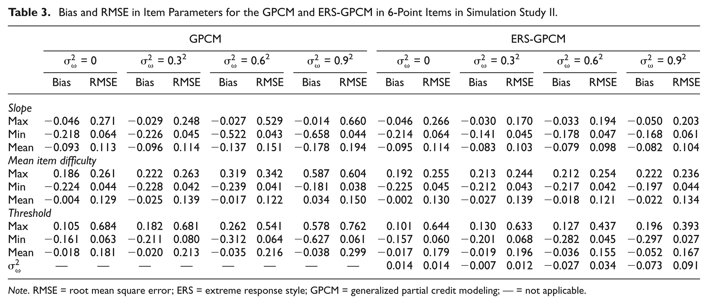
Study II focused on the consequences of model misspecification. It had two conditions: (a) the ERS-GPCM was fit to GPCM data (without ERS) and (b) the GPCM was fit to ERS-GPCM data (ERS ignored). Other settings included 40 six-point items answered by 1,000 persons, and $σ_{ω}^{2} = 0,$ 0.3², 0.6², and 0.9². When $σ_{ω}^{2} = 0,$ the GPCM and ERS-GPCM were actually equivalent. A total of 20 replications were conducted.

Analysis

The following priors were used in WinBUGS: N(0, 10) for the item difficulties and threshold difficulties, log-normal (0, 1) for item slopes, and gamma (1, 0.1) for the inverse of $σ_{ω}^{2} .$ The first 5,000 iterations were discarded for burn-in, and the subsequent 5,000 iterations were retained. Parameter estimates were sampled from the remaining iterations per 10 values. The bias and root mean square error (RMSE) of parameter estimates were computed, and the deviance information criterion (DIC) was used to compare models in Study II.

Results

Study I

Tables 1 and 2 summarize the bias and RMSE values for 4- and 6-point items, respectively. The item parameter estimates for the overall difficulties and thresholds were seriously biased in small sample sizes (N = 250); fortunately, when the sample size or test length increased, the estimation gradually improved. It appeared that $σ_{ω}^{2}$ was consistently underestimated, but the estimate was close to the true value in large sample sizes and long tests. A comparison of Tables 1 and 2 revealed that the estimation for ERS was improved with 6-point items. In general, the parameter recovery of the ERS-GPCM, although not excellent, was satisfactory in large datasets.

Table 1.

Bias and RMSE in Item Parameters for the ERS-GPCM in 4-Point Items in Simulation Study I.

	20 Items								40 Items
	N = 250		N = 500		N = 1,000		N = 2,000		N = 250		N = 500		N = 1,000		N = 2,000
	Bias	RMSE	Bias	RMSE	Bias	RMSE	Bias	RMSE	Bias	RMSE	Bias	RMSE	Bias	RMSE	Bias	RMSE
Slope
Max	−0.045	0.255	0.054	0.379	−0.008	0.169	0.003	0.113	−0.072	0.373	−0.049	0.293	−0.031	0.167	−0.011	0.104
Min	−0.169	0.086	−0.127	0.071	−0.071	0.059	−0.041	0.032	−0.300	0.097	−0.231	0.085	−0.111	0.056	−0.064	0.034
Mean	−0.096	0.163	−0.054	0.140	−0.034	0.089	−0.015	0.054	−0.188	0.229	−0.103	0.144	−0.065	0.096	−0.033	0.062
Mean difficulty
Max	0.511	0.617	0.166	0.381	0.142	0.187	0.024	0.128	0.635	0.770	0.261	0.388	0.154	0.204	0.085	0.150
Min	−0.271	0.105	−0.291	0.049	−0.058	0.042	−0.065	0.028	−0.501	0.138	−0.281	0.041	−0.121	0.041	−0.078	0.029
Mean	0.081	0.305	0.009	0.170	0.023	0.087	−0.009	0.058	0.049	0.342	−0.006	0.173	0.002	0.104	0.003	0.071
Threshold
Max	0.085	0.553	0.069	0.418	0.042	0.185	0.019	0.166	0.104	0.684	0.136	0.319	0.041	0.183	0.035	0.134
Min	−0.230	0.137	−0.169	0.079	−0.074	0.058	−0.041	0.033	−0.297	0.134	−0.170	0.065	−0.091	0.045	−0.057	0.039
Mean	−0.072	0.309	−0.024	0.175	−0.012	0.106	−0.009	0.078	−0.087	0.303	−0.044	0.178	−0.026	0.109	−0.012	0.077
$σ_{ω}^{2}$	−0.063	0.071	−0.035	0.044	−0.022	0.039	−0.008	0.026	−0.055	0.058	−0.036	0.040	−0.020	0.025	−0.011	0.018

Note. RMSE = root mean square error; ERS = extreme response style; GPCM = generalized partial credit modeling.

Table 2.

Bias and RMSE in Item Parameters for the ERS-GPCM in 6-Point Items in Simulation Study I.

	20 Items								40 Items
	N = 250		N = 500		N = 1,000		N = 2,000		N = 250		N = 500		N = 1,000		N = 2,000
	Bias	RMSE	Bias	RMSE	Bias	RMSE	Bias	RMSE	Bias	RMSE	Bias	RMSE	Bias	RMSE	Bias	RMSE
Slope
Max	−0.108	0.358	−0.041	0.300	−0.033	0.144	0.001	0.089	−0.144	0.489	−0.077	0.396	−0.042	0.191	−0.025	0.106
Min	−0.308	0.134	−0.186	0.065	−0.127	0.059	−0.056	0.023	−0.451	0.154	−0.356	0.091	−0.151	0.052	−0.083	0.039
Mean	−0.193	0.235	−0.091	0.130	−0.064	0.098	−0.020	0.051	−0.270	0.288	−0.160	0.179	−0.091	0.109	−0.047	0.065
Item difficulty
Max	0.534	0.577	0.250	0.331	0.161	0.267	0.047	0.112	0.761	0.847	0.403	0.424	0.200	0.285	0.112	0.143
Min	−0.464	0.084	−0.245	0.055	−0.138	0.040	−0.066	0.028	−0.782	0.087	−0.388	0.077	−0.264	0.036	−0.121	0.025
Mean	0.044	0.284	0.014	0.157	0.006	0.107	−0.006	0.057	0.072	0.400	−0.054	0.245	−0.027	0.118	−0.004	0.071
Threshold
Max	0.447	1.021	0.193	0.886	0.110	0.553	0.221	0.370	0.449	1.197	0.256	0.741	0.234	0.508	0.098	0.305
Min	−0.462	0.180	−0.307	0.074	−0.117	0.057	−0.103	0.035	−0.623	0.098	−0.446	0.110	−0.262	0.073	−0.101	0.040
Mean	−0.038	0.387	−0.022	0.233	−0.015	0.152	−0.003	0.111	−0.081	0.462	−0.052	0.291	−0.025	0.172	−0.013	0.107
$σ_{ω}^{2}$	−0.045	0.052	−0.032	0.043	−0.015	0.022	−0.010	0.018	−0.029	0.041	−0.024	0.031	−0.012	0.017	−0.007	0.012

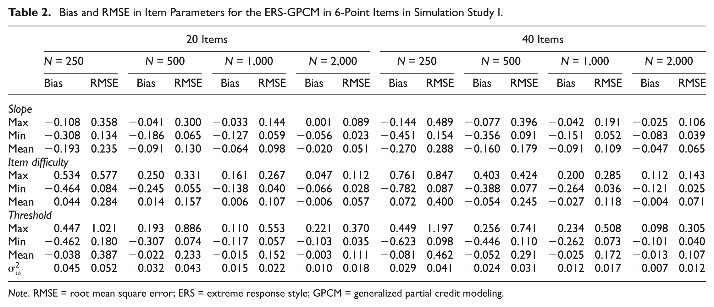
Note. RMSE = root mean square error; ERS = extreme response style; GPCM = generalized partial credit modeling.

Study II

Table 3 summarizes the bias and RMSE values when the GPCM and ERS-GPCM were fit to 6-point items. When $σ_{ω}^{2} = 0,$ both models yielded similar results. Besides, $σ_{ω}^{2}$ estimated by the ERS-GPCM was very close to its true value of zero (RMSE = 0.014). In other words, it did little harm to fit a necessarily complicated model (i.e., ERS-GPCM) to data without ERS (i.e., GPCM). When $σ_{ω}^{2} \neq 0,$ indicating there was ERS, the ERS-GPCM could recover the parameters fairly well, whereas the GPCM yielded very poor estimation. For example, when the ERS-GPCM was fit, the RMSE for the slope parameters was 0.103, 0.098, and 0.104, when $σ_{ω}^{2} =$ 0.3², 0.6², and 0.9², respectively; when GPCM was fit, the RMSE became 0.114, 0.151, and 0.194, respectively. The larger the $σ_{ω}^{2},$ the worse the GPCM performed as compared with the ERS-GPCM. The same findings applied to the mean item difficulty parameters and the threshold parameters.

Table 3.

Bias and RMSE in Item Parameters for the GPCM and ERS-GPCM in 6-Point Items in Simulation Study II.

	GPCM								ERS-GPCM
	$σ_{ω}^{2}$ = 0		$σ_{ω}^{2}$ = 0.3²		$σ_{ω}^{2}$ = 0.6²		$σ_{ω}^{2}$ = 0.9²		$σ_{ω}^{2}$ = 0		$σ_{ω}^{2}$ = 0.3²		$σ_{ω}^{2}$ = 0.6²		$σ_{ω}^{2}$ = 0.9²
	Bias	RMSE	Bias	RMSE	Bias	RMSE	Bias	RMSE	Bias	RMSE	Bias	RMSE	Bias	RMSE	Bias	RMSE
Slope
Max	−0.046	0.271	−0.029	0.248	−0.027	0.529	−0.014	0.660	−0.046	0.266	−0.030	0.170	−0.033	0.194	−0.050	0.203
Min	−0.218	0.064	−0.226	0.045	−0.522	0.043	−0.658	0.044	−0.214	0.064	−0.141	0.045	−0.178	0.047	−0.168	0.061
Mean	−0.093	0.113	−0.096	0.114	−0.137	0.151	−0.178	0.194	−0.095	0.114	−0.083	0.103	−0.079	0.098	−0.082	0.104
Mean item difficulty
Max	0.186	0.261	0.222	0.263	0.319	0.342	0.587	0.604	0.192	0.255	0.213	0.244	0.212	0.254	0.222	0.236
Min	−0.224	0.044	−0.228	0.042	−0.239	0.041	−0.181	0.038	−0.225	0.045	−0.212	0.043	−0.217	0.042	−0.197	0.044
Mean	−0.004	0.129	−0.025	0.139	−0.017	0.122	0.034	0.150	−0.002	0.130	−0.027	0.139	−0.018	0.121	−0.022	0.134
Threshold
Max	0.105	0.684	0.182	0.681	0.262	0.541	0.578	0.762	0.101	0.644	0.130	0.633	0.127	0.437	0.196	0.393
Min	−0.161	0.063	−0.211	0.080	−0.312	0.064	−0.627	0.061	−0.157	0.060	−0.201	0.068	−0.282	0.045	−0.297	0.027
Mean	−0.018	0.181	−0.020	0.213	−0.035	0.216	−0.038	0.299	−0.017	0.179	−0.019	0.196	−0.036	0.155	−0.052	0.167
$σ_{ω}^{2}$	—	—	—	—	—	—	—	—	0.014	0.014	−0.007	0.012	−0.027	0.034	−0.073	0.091

Note. RMSE = root mean square error; ERS = extreme response style; GPCM = generalized partial credit modeling; — = not applicable.

Of the 20 replications, the DIC favored the GPCM 15, 0, 0, and 0 times, respectively, when $σ_{ω}^{2} =$ 0, 0.3², 0.6², and 0.9². When $σ_{ω}^{2} = 0,$ the GPCM was the true model; when $σ_{ω}^{2} \neq 0,$ the ERS-GPCM was the true model. It appeared that the DIC performed fairly well in the selection of true models. Next, consider the test reliability estimates obtained from the two models. In the ERS-GPCM, on average the test reliability estimates were .968, .963, .963, and .960, respectively, when $σ_{ω}^{2} = 0,$ 0.3², 0.6², and 0.9². In the GPCM, on average the test reliability estimates were .968, .964, .966, and .966, respectively, when $σ_{ω}^{2} = 0,$ 0.3², 0.6², and 0.9². Treating the ERS-GPCM as a gold standard (because it was the data-generating model), it appeared that the GPCM tended to slightly overestimate the test reliability.

Two Empirical Examples

Example I: Interpersonal Conflicts

Lo (2001) developed a scale to measure interpersonal conflicts, which consisted of 20 seven-point items: 1 = strongly unconfident, 4 = neutral, 7 = strongly confident. After removing a few invalid cases with unknown demographic variables, 982 students were kept in the analyses. Six IRT models were fit: (a) PCM, (b) ERS-PCM, (c) ERS-PCM-c, (d) GPCM, (e) ERS-GPCM, and (f) ERS-GPCM-c. The ERS-PCM-c and the ERS-GPCM-c included gender (male = 0 and female = 1) and number of siblings as the covariates of ω (see Equation 16).

The DIC values for the six models were 67,170, 64,946, 64,830, 67,063, 64,896, and 64,798, respectively, suggesting the ERS-GPCM-c had the best fit. In other words, adding slope parameters and covariates was useful. In the ERS-GPCM-c, the test reliability was 0.82; the estimates and standard errors (in parentheses) for the regression coefficients κ_gender and κ_sibling on ω were 0.001 (0.082) and −0.187 (0.028), respectively, and the residual variance was 1.098 (0.107). Thus, it can be concluded that these students showed different degrees of ERS; no gender difference was observed regarding ERS, but the number of siblings was a significant predictor of ERS: the more siblings one had, the more likely he or she would endorse extreme responses. This might be because a teenager with more siblings has more experience with interpersonal conflicts, so that his or her endorsement would be more highly differentiated.

Table 4 lists the raw responses of nine students and their θ and ω estimates. Students 19, 771, and 790 all had the same mean item score of 2.80, a very different SD of 1.28, 1.64, and 2.65, respectively, and a very different number of extreme responses (options of 1 and 7) of 4, 6, and 18, respectively. Because their mean item scores were identical, their θ estimates were expected to be very similar under the GPCM: −1.47, −1.54, and −1.70, respectively. Because Student 790 tended to choose extreme options (in this case, many 1s), it was very likely that his or her true θ value was not as low as the mean raw score indicated. So the ERS-GPCM-c gave this student an upward estimation on θ from −1.70 to −1.32. To be balanced, the ERS-GPCM-c gave Student 19 a downward estimation on θ from −1.47 to −1.66.

Table 4.

Students’ Response Patterns and the Estimates for θ and ω (SE in Parentheses) in Example 1.

					GPCM	ERS-GPCM-c
Student ID	Raw responses	Mean	SD	#ER	$\hat{θ}$	$\hat{θ}$	$\hat{ω}$
19	45333412211244442214	2.80	1.28	4	−1.47 (0.37)	−1.66 (0.50)	0.95 (0.41)
771	54121534211321641253	2.80	1.64	6	−1.54 (0.38)	−1.42 (0.42)	0.51 (0.30)
790	41141771111177711111	2.80	2.65	18	−1.70 (0.38)	−1.32 (0.36)	0.14 (0.09)
665	43454434433353444534	3.80	0.70	0	−0.49 (0.38)	−0.77 (0.54)	2.57 (0.68)
807	43343214643435543645	3.80	1.24	1	−0.40 (0.38)	−0.48 (0.42)	1.47 (0.46)
232	75737765224114723111	3.80	2.40	10	−0.72 (0.37)	−0.70 (0.31)	0.23 (0.14)
145	55646666467777664656	5.75	0.97	4	1.59 (0.43)	1.88 (0.59)	1.04 (0.45)
387	54364776767777744755	5.75	1.37	9	1.49 (0.43)	1.58 (0.54)	0.75 (0.39)
729	67537767777673374457	5.75	1.55	10	1.57 (0.42)	1.29 (0.40)	0.28 (0.19)

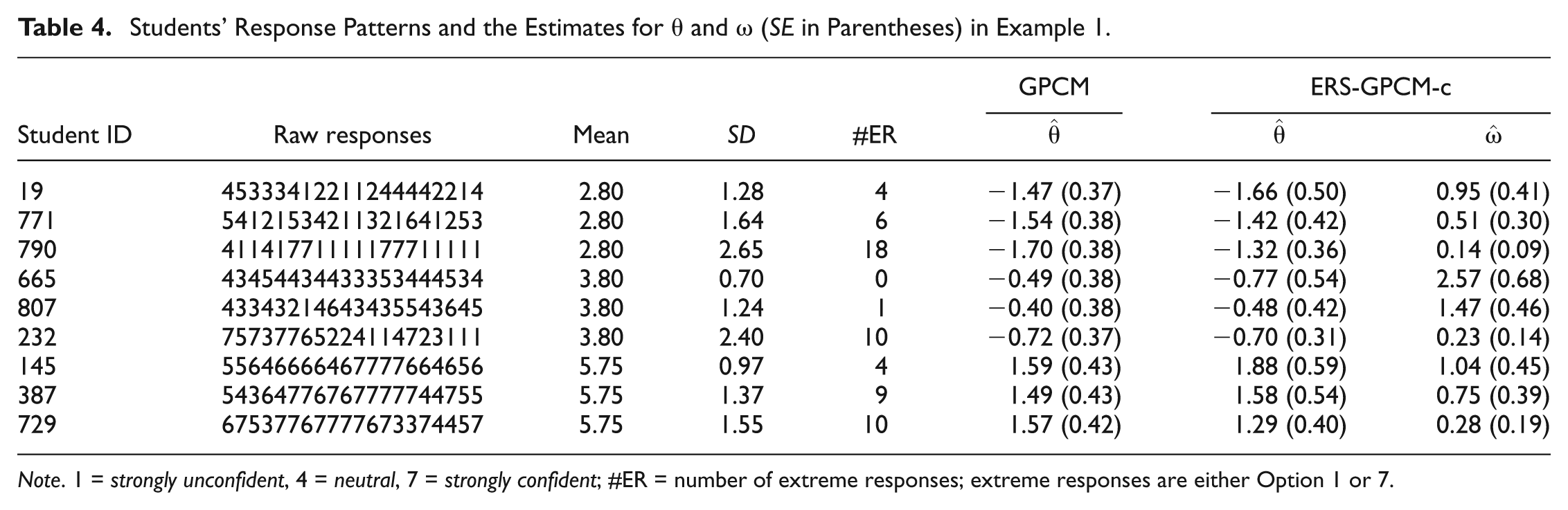
Note. 1 = strongly unconfident, 4 = neutral, 7 = strongly confident; #ER = number of extreme responses; extreme responses are either Option 1 or 7.

The case of Students 145, 387, and 729 was the opposite. Among the three students, Student 145 exhibited the least ERS ( $\hat{ω} = 1.04$ ), and Student 729 exhibited the most ERS ( $\hat{ω} = 0.28$ ). Because Student 729 tended to choose extreme options (in this case, many 7s), it was very likely that his or her true θ value was not as high as the mean raw score indicated. So the ERS-GPCM-c gave this student a downward estimation on θ from 1.57 to 1.29. To be balanced, the ERS-GPCM-c gave Student 145 an upward estimation on θ from 1.59 to 1.88.

Figure 3 describes the relationship of the θ estimates obtained from the ERS-GPCM-c and GPCM. Some variations were found. The difference in the θ estimates between models ranged from −0.95 to 0.93, with a mean of −0.0004 and an SD of 0.22. The correlation was 0.97, which was reasonable because only 30% of students had a ω estimate that was statistically significant.

Figure 3.

Relationship in the θ estimates between the ERS-GPCM-c and GPCM of Example 1.

Example II: ICCS 2009

The International Civic and Citizenship Education Study (ICCS) surveyed students’ preparation in undertaking the role of citizens. In 2009, in addition to the common instrument, ICCS included regional modules for Europe, Latin America, and Asia. The Latin American module had a scale measuring students’ perception of government and law. That scale consisted of three subscales measuring students’ attitudes toward authoritarianism in government (9 items), corrupt practices in government (6 items), and disobeying the law (11 items). Students were asked to indicate their level of agreement with the statements (1 = strongly disagree, 2 = disagree, 3 = agree, 4 = strongly agree). A higher score denoted a greater degree of acceptance of a specific undemocratic activity. Because these three subscales were moderately to highly correlated (Schulz, Ainley, & Fraillon, 2011), we adopted the multidimensional approach to analyze them simultaneously (Cheng et al., 2009). We followed the normal practice of fitting the ICCS data with the family of Rasch models (Schulz et al., 2011). As pointed out in the official report, the correlations among the target three latent traits were rather strong, ranging from 0.72 to 0.86. Thus, the multidimensional form of the partial credit model (MPCM) and the multidimensional form of the ERS-PCM (MERS-PCM; Equation 14) were fit. A total of 5,626 cases in Mexico were analyzed. WinBUGS was used to calibrate the parameters.

The DIC values for the MPCM and MERS-PCM were 306,893 and 277,422, respectively, suggesting the MERS-PCM had a better fit. In the MERS-PCM, the test reliabilities for the three θ variables were 0.85, 0.84, and 0.82, respectively, whereas the test reliabilities in the MPCM were 0.89, 0.88, and 0.86, respectively, suggesting that ignoring ERS by fitting standard IRT models overestimates the precision of the measurement, which is consistent with the findings of previous simulation studies. The estimate for $σ_{ω}^{2}$ was 1.43, suggesting that the Mexican students showed very different degrees of ERS. A nonlinear relationship between ω and the SD of item scores and the number of extreme responses is shown in Figure 4. As expected, a lower ω corresponded to more frequent extreme responses.

Figure 4.

Scatter plots of the θ and ω estimates, the mean and SD of raw item scores, and the number of extreme responses (#ER) of Example 2.

The assumption of a common ω for ERS across the three subscales, as adopted in the MERS-PCM, can be relaxed by allowing a distinct ω for each subscale, as shown in Equation (12). This general and complicated model was fit to the data and compared with the MERS-PCM. Although the DIC preferred the complicated model, the practical difference between these two models was minimal. Specifically, in the complicated model the three ω estimates (in logarithm scale) were highly correlated (0.81 < r < 0.92), suggesting a single ω might be enough. The estimates for the item difficulties and thresholds obtained from the two models were almost perfectly correlated (r = 0.999); the largest difference in the test reliabilities of the θ variable for the three subscales obtained from the two models was as small as 0.01. Besides, on average, the standard errors for the three ω estimates in the complicated model were 55% larger than those for the single ω estimate in the MERS-PCM. In view of these results, the simpler MERS-PCM was kept.

Conclusion and Discussion

Respondents may exhibit different response styles when responding to Likert-type or rating-scale items. Some respondents may prefer extreme options, whereas others prefer middle options. To model this kind of personal preference, we developed a new class of ERS models where a random-effect variable is added to standard IRT models to account for the random widths between thresholds across respondents so that the degrees of ERS can be quantified. Two simulation studies were conducted to assess parameter recovery and the effect of model misspecification. The results showed that the parameters in the ERS models could be recovered fairly well using WinBUGS. Even when respondents did not exhibit ERS, fitting the ERS models still yielded good parameter recovery. In contrast, ignoring ERS by fitting standard IRT models yielded biased estimation, and the larger the variation of ERS the more serious the biased estimation. Moreover, ignoring ERS resulted in overestimated test reliability. Finally, the DIC appeared to be very powerful in selecting true models.

In the simulation study, we deliberately increased the test length to 20 or 40 items to yield a better estimation of ω. In general, the longer the test, the better the estimation of person parameters (i.e., θ and ω in this study). To gain a precise estimate for ω, either the test should be long or the number of options in each item should be large. Furthermore, compared with standard IRT models, the ERS models require a larger sample size for the parameter estimation, mainly because of the model complexity.

This study focuses on ERS and does not consider other types of response styles, which are left for future studies. For instance, previous studies have investigated acquiescent and disacquiescent response styles within the non-IRT framework (Johnson et al., 2005; Kieruj & Moors, 2010; van Herk et al., 2004; Weijters et al., 2008). Future studies can aim to develop IRT models to account for these response styles. Recently, researchers have developed IRT-based sequential decision models to describe response styles in which observed responses are regarded as branched outcomes of multiple response processes. For example, Böckenholt (2012) developed a branching IRT model for odd numbers of categories, in which three branching processes are posited in responding to Likert-type scales. For example, in responding to a 5-point Likert-type scale (strongly disagree, disagree, neutral, agree, and strongly agree), the sequential binary judgment involves: (a) endorsing the neutral opinion or not; (b) if the nonneutral opinion is preferred, choosing the direction of opinion (disagree vs. agree); and (c) expressing the intensity of the opinion (strongly or not). Similarly, Thissen-Roe and Thissen (2013) introduce a two-decision model to describe extreme response sets, in which the first and second stages of Böckenholt’s (2012) model are combined and the third stage is expanded to cover the neutral option. Although these approaches destroy the ordering of categories in Likert-type or rating-scale items, the response styles appear to be better examined. How these approaches would work on other response styles needs further investigation.

Footnotes

Declaration of Conflicting Interests

The author(s) declared no potential conflicts of interest with respect to the research, authorship, and/or publication of this article.

Funding

The author(s) received no financial support for the research, authorship, and/or publication of this article.

References

Adams

R. J.

Wilson

Wang

W.-C.

(1997). The multidimensional random coefficients multinomial logit model. Applied Psychological Measurement, 21, 1-23.

Adams

R. J.

Wilson

(1997). Multilevel item response models: An approach to errors in variables regression. Journal of Educational and Behavioral Statistics, 22, 47-76.

Alexeev

Templin

Cohen

A. S.

(2011). Spurious latent classes in the mixture Rasch model. Journal of Educational Measurement, 48, 313-332.

Andrich

(1978). A rating formulation for ordered response categories. Psychometrika, 43, 561-573.

Arce-Ferrer

A. J.

(2006). An investigation into the factors influencing extreme-response style: Improving meaning of translated and culturally adapted rating scales. Educational and Psychological Measurement, 66, 374-392.

Baumgartner

Steenkamp

J.-B. E. M.

(2001). Response styles in marketing research: A cross-national investigation. Journal of Marketing Research, 38, 143-156.

Böckenholt

(2012). Modeling multiple response processes in judgment and choice. Psychological Methods, 17, 665-678.

Bolt

D. M.

Johnson

T. R.

(2009). Addressing score bias and differential item functioning due to individual differences in response style. Applied Psychological Measurement, 33, 335-352.

Bolt

D. M.

Newton

J. R.

(2011). Multiscale measurement of extreme response style. Educational and Psychological Measurement, 71, 814-833.

10.

Chen

Lee

S.-Y.

Stevenson

H. W.

(1995). Response style and cross-cultural comparisons of rating scales among East Asian and North American students. Psychological Science, 6, 170-175.

11.

Cheng

Y.-Y.

Wang

W.-C.

Y.-H.

(2009). Multidimensional Rasch analysis of a psychological test with multiple subtests: A statistical solution for the bandwidth-fidelity dilemma. Educational and Psychological Measurement, 69, 369-388.

12.

Curtis

S. M.

(2010). BUGS code for item response theory. Journal of Statistical Software, 36(1), 1-34.

13.

De Beuckelaer

Weijters

Rutten

(2010). Using ad hoc measures for response styles: A cautionary note. Quality & Quantity, 44, 761-775.

14.

de Jong

M. G.

Steenkamp

J.-B. E. M.

Fox

J.-P.

Baumgartner

(2008). Using item response theory to measure extreme response style in marketing research: A global investigation. Journal of Marketing Research, 45, 104-115.

15.

Embretson

S. E.

Reise

S. P.

(2000). Item response theory for psychologists. Mahwah, NJ: Erlbaum.

16.

Greenleaf

E. A.

(1992). Measuring extreme response style. Public Opinion Quarterly, 56, 328-351.

17.

Hamilton

D. L.

(1968). Personality attributes associated with extreme response style. Psychological Bulletin, 69, 192-203.

18.

Hurley

J. R.

(1998). Timidity as a response style to psychological questionnaires. Journal of Psychology, 132, 201-210.

19.

Jackson

D. N.

Messick

(1958). Content and style in personality assessment. Psychological Bulletin, 55, 243-252.

20.

Javaras

K. N.

Ripley

B. D.

(2007). An “unfolding” latent variable model for Likert attitude data. Journal of the American Statistical Association, 102, 454-463.

21.

Johnson

T. R.

(2003). On the use of heterogeneous thresholds ordinal regression models to account for individual differences in response style. Psychometrika, 68, 563-583.

22.

Johnson

T. R.

Bolt

D. M.

(2010). On the use of factor-analytic multinomial logit item response models to account for individual differences in response style. Journal of Educational and Behavioral Statistics, 35, 92-114.

23.

Johnson

T. R.

Kulesa

Llc

Cho

Y. I.

Shavitt

(2005). The relation between culture and response styles: Evidence from 19 countries. Journal of Cross-Cultural Psychology, 36, 264-277.

24.

Kieruj

N. D.

Moors

(2010). Variations in response style behavior by response scale format in attitude research. International Journal of Public Opinion Research, 22, 320-342.

25.

K.-Y.

(2001). Interpersonal harmony and the values of forbearance: Understanding generation gap through interpersonal conflicts (NSC Research Report No. NSC90-2413-H-031-006-SSS). Taipei, Taiwan: National Science Council.

26.

Luo

(2001). A class of probabilistic unfolding models for polytomous responses. Journal of Mathematical Psychology, 45, 224-248.

27.

Masters

(1982). A Rasch model for partial credit scoring. Psychometrika, 47, 149-174.

28.

Moors

(2008). Exploring the effect of a middle response category on response style in attitude measurement. Quality & Quantity, 42, 779-794.

29.

Muraki

(1992). A generalized partial credit model: Application of an EM algorithm. Applied Psychological Measurement, 16, 159-176.

30.

Naemi

B. D.

Beal

D. J.

Payne

S. C.

(2009). Personality predictors of extreme response style. Journal of Personality, 77, 261-286.

31.

Rorer

L. G.

(1965). The great response-style myth. Psychological Bulletin, 63, 129-156.

32.

Rost

Carstensen

von Davier

(1997). Applying the mixed Rasch model to personality questionnaires. In Rost

Langeheine

(Eds.), Applications of latent trait and latent class models in the social sciences (pp. 324-332). New York, NY: Waxmann.

33.

Samejima

(1969). Estimation of latent ability using a response pattern of graded scores. Psychometrika Monograph Supplement, 34, 100-114.

34.

SAS Institute. (1999). The NLMIXED procedure [Computer program]. Cary, NC: Author.

35.

Schulz

Ainley

Fraillon

(Eds.). (2011). ICCS 2009 Technical Report. Amsterdam, Netherlands: International Association for the Evaluation of Educational Achievement.

36.

Spiegelhalter

D. J.

Thomas

Best

Lunn

(2007). WinBUGS version 1.4.3. Cambridge, England: MRC Biostatistics Unit, Institute of Public Health.

37.

Thissen-Roe

Thissen

(2013). A two-decision model for responses to Likert-type items. Journal of Educational and Behavioral Statistics. Advance online publication. 10.3102/1076998613481500

38.

van Herk

Poortinga

Y. H.

Verhallen

T. M. M.

(2004). Response styles in rating scales: Evidence of method bias in data from six EU countries. Journal of Cross-Cultural Psychology, 35, 346-360.

39.

van Rosmalen

van Herk

Groenen

P. J. F.

(2010). Identifying response styles: A latent-class bilinear multinomial logit model. Journal of Marketing Research, 47, 157-172.

40.

Van Vaerenbergh

Thomas

T. D.

(2013). Response styles in survey research: A literature review of antecedents, consequences, and remedies. International Journal of Public Opinion Research, 25, 195-217.

41.

von Davier

Eid

Zickar

M. J.

(2007). Detecting response styles and faking in personality and organizational assessments by mixed Rasch models. In Carstensen

C. H.

(Ed.), Multivariate and mixture distribution Rasch models (pp. 255-270). New York, NY: Springer.

42.

Wang

W.-C.

Wilson

Shih

C.-L.

(2006). Modeling randomness in judging rating scales with a random-effects rating scale model. Journal of Educational Measurement, 43, 335-353.

43.

Wang

W.-C.

S.-L.

(2011). The random-effect generalized rating scale model. Journal of Educational Measurement, 48, 441-456.

44.

Weijters

Geuens

Schillewaert

(2010). The stability of individual response styles. Psychological Methods, 15, 96-110.

45.

Weijters

Schillewaert

Geuens

(2008). Assessing response styles across modes of data collection. Journal of the Academy of Marketing Science, 36, 409-422.