
Abstract
The standardized mean difference (SMD) is perhaps the most important meta-analytic effect size. It is typically used to represent the difference between treatment and control population means in treatment efficacy research. It is also used to represent differences between populations with different characteristics, such as persons who are depressed and those who are not. Measurement error in the independent variable (IV) attenuates SMDs. In this article, we derive a formula for the SMD that explicitly represents accuracy of classification of persons into populations on the basis of scores on an IV. We suggest an alternate version of the SMD less vulnerable to measurement error in the IV. We derive a novel approach to correcting the SMD for measurement error in the IV and show how this method can also be used to reliability correct the unstandardized mean difference. We compare this reliability correction approach with one suggested by Hunter and Schmidt in a series of Monte Carlo simulations. Finally, we consider how the proposed reliability correction method can be used in meta-analysis and suggest future directions for both research and further theoretical development of the proposed reliability correction method.
Keywords
The standardized mean difference (SMD) is one of the most important effect sizes in meta-analysis. The SMD is a two variable effect size (EFS) used to compare the means of different populations on a dependent variable (DV), with population membership indicated by a dichotomous independent variable (IV), neither of which may be measured the same across studies. The SMD is commonly used to represent outcomes in research examining the efficacy of psychological, educational, and medical interventions and treatments (Borenstein, Hedges, Higgins, & Rothstein, 2009; Lipsey &Wilson, 2001). The SMD is also used to represent differences on a DV between populations composed of persons with different characteristics (Grissom & Kim, 2011), such as males and females in gender differences research (Hedges & Olkin, 1985), and differences between persons who are depressed and those who are not (e.g., Snyder, 2013).
A number of artifact adjustments have been suggested for EFSs in meta-analysis (Hunter & Schmidt, 2004; Schmidt, Le, & Oh, 2009). Lipsey and Wilson (2001) suggest the most useful are corrections for the effects of measurement error. While the effects of measurement error in the DV on the SMD are commonly addressed (e.g., Hedges & Olkin, 1985; Lipsey & Wilson, 2001), the effects of measurement error in the IV are less frequently considered. Hunter and Schmidt (2004), in perhaps the most extensive consideration of this topic, observed that measurement error in the IV: (a) decreases the difference between the population means in the numerator of the SMD and (b) increases the within population variances of scores on the DV in the denominator of the SMD, causing attenuation of the SMD.
The attenuation of SMDs because of measurement error in the IV can have deleterious effects on meta-analysis (Orwin & Cordray, 1985). If different measures of the IV, with differing levels of measurement error, are used in a series of studies, the SMDs for these studies will have differential levels of attenuation. This differential attenuation will propagate through meta-analyses. For example, tests of homogeneity will be affected. A test of homogeneity of differentially attenuated SMDs can suggest heterogeneity, even when the set of SMDs free of the effects of measurement error are truly homogeneous (Hedges & Olkin, 1985). Correlations between differentially attenuated SMDs and explanatory variables will also be attenuated, affecting meta-regression analyses. These considerations underscore the importance of development and use of methods for disattenuating the SMD for the effects of measurement error in the IV (Hedges & Olkin, 1985).
Hunter and Schmidt (2004) sketched a method for correcting the SMD for the effects of measurement error in the IV based on the classical theory correction for attenuation and formulas for converting the SMD to the point–biserial correlation, and vice versa. This approach could be implemented as in the following example. Suppose a researcher is interested in the relationship between major depressive disorder (MDD) and cognitive deficits (Snyder, 2013). The 1-year prevalence of MDD in the United States is about .09 (Kazdin, 2002). Assume the interview procedure used to classify persons as having, or not having, MDD has sensitivity .717 and specificity .90, mean values for interview methods from a recent review (Swedish Council on Health Technology Assessment, 2012). These sensitivity and specificity values, combined with the prevalence of .09, imply at the population level 84.5% of persons will be classified as not having, and 15.5% as having, MDD (Pepe, 2003); and imply the square root of the reliability coefficient for classifications based on scores from this IV will be about .487 (Phi correlation between observed and true classification; Nunnally, 1978).
Assume in the researcher’s study 84.5% of participants are classified as not having, and 15.5% as having, MDD; that the difference between the group means on the DV for those with MDD and those without is +1.95; and the variances of scores on the DV are equal to 109.2 in both MDD and non-MDD groups. The researcher computes the sample SMD, obtaining .187, and then converts this to a point–biserial correlation using formula 3.34 in Lipsey and Wilson (2001), obtaining a value of .067. This is divided by .487 (Hunter and Schmidt, 2004), giving a reliability corrected point–biserial of .139. This is transformed back to a SMD using formula 3.36 from Lipsey and Wilson (2001), giving a reliability corrected SMD of .387. A little algebra shows the reliability corrected SMD obtained using this three step procedure can be condensed into the formula,
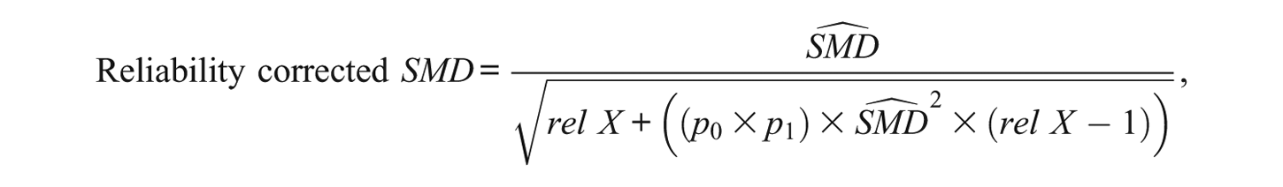
where
In this article, we focus on correcting the SMD in meta-analysis for measurement error in the IV. We expand on Hunter and Schmidt’s (2004) examination of the effects of measurement error in the IV on the SMD, and their development of methodology for correcting the SMD for this error. We first conceptualize and formalize measurement of an IV used to classify persons into different populations with respect to their possession of a characteristic of interest, such as depression. We derive a formula for the population SMD that includes representation, in both numerator and denominator, of the accuracy of classification of persons, and which explicitly represents attenuation of the numerator because of measurement error in the IV. We then use a model-based simulation (Axelrod, 2007; Banks, 2009) to examine the effects, on the SMD, of misclassification of persons into populations. The results elaborate Hunter and Schmidt’s (2004) observations, showing measurement error in the IV can attenuate the SMD to a greater degree than measurement error in the DV. We next propose a novel method for disattenuating the SMD for the effects of measurement error in the IV. We compare this proposed method with the method described by Hunter and Schmidt in a series of Monte Carlo simulations. We conclude by considering the following:
How the proposed method can be used in meta-analysis
Further theoretical development of the proposed reliability correction method
Implications of the results of the Monte Carlo simulations for future research on the proposed reliability correction method
Measurement of an IV for Classification
True Population Membership
Individuals are classified into populations based on measurement of an IV. The IV is measured and persons classified, based on IV scores, into different populations. Figure 1 helps conceptualize this measurement. At the top of this figure are two populations,
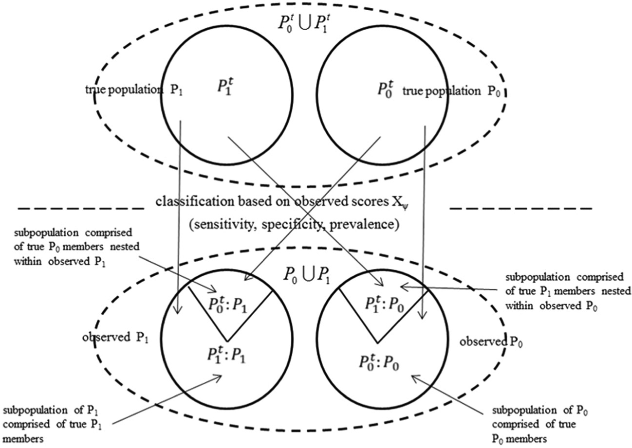
Illustration of “true populations”
Observed Population Membership
In practice, persons from
Population and Subpopulation Means and Variances
The symbol
Reliability of Classification
Hunter and Schmidt (2004) noted that appropriate reliability coefficients need to be used when correcting EFSs for measurement error. The classical reliability coefficient can be misleading for representing measurement error when scores are used for classification. In this case “reliability” is better represented by quantities indicating classification accuracy (Berk, 1980; Brennan, 2001; Divgi, 1980; Haertel, 2006; Kane & Brennan, 1980). Two population specific indices for representing classification accuracy are the sensitivity, or true positive fraction (TPF), and the specificity, or true negative fraction (TNF) (Pepe, 2003). The sensitivity,

the conditional probability a person is correctly identified as possessing the characteristic of interest using the scores

the conditional probability a person is correctly identified as not possessing the characteristic of interest using the scores
Two other indices indicate the accuracy of classification into
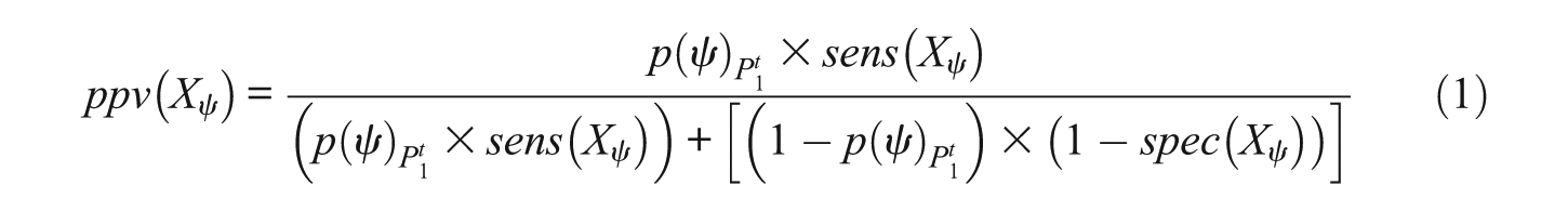
is the positive predictive value (PPV) of classification of persons into
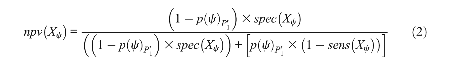
is the negative predictive value, NPV, of classification of persons into
Misclassification Due Only to Random Measurement Error
Assume misclassification of persons into
Thus, persons who are members of
Equality of Collective Populations
and
Consider again Figure 1. The persons in
Two Versions of the Population SMD
The “Common” Population SMD
The population SMD is traditionally defined as the difference between the means of populations
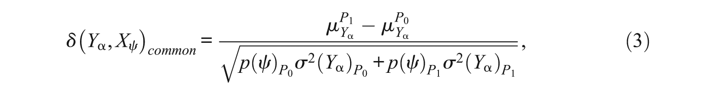
where

is the proportion from
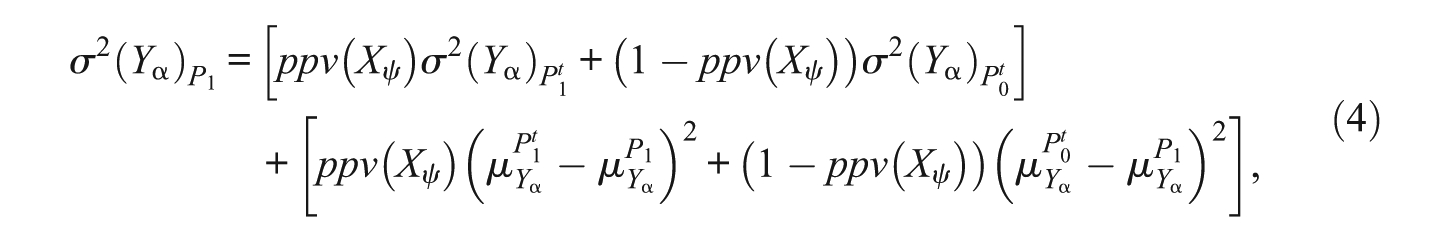
and the variance
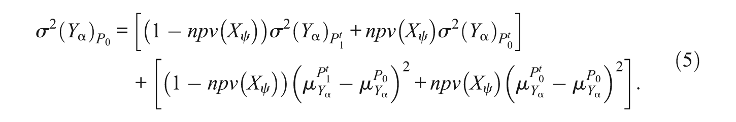
The perhaps complex symbolism for the common population SMD is used to indicate it is based on observed scores
As proven in the appendix, the numerator in Equation (3) can be expressed as
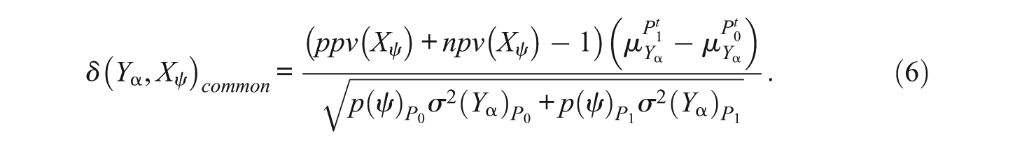
The common SMD expressed by Equations (3) through (6) formalizes observations of Hunter and Schmidt (2004). The effects of measurement error in the IV on both numerator and denominator are explicitly represented by
An Alternate Version of the Population SMD
The use of SDs other than that in the denominator of the common SMD has been suggested. For example, the SD of scores on the DV in the control group in studies of treatment efficacy has been suggested (Hunter & Schmidt, 2004). An alternative with important advantages is the SD of scores on the DV in the combined population
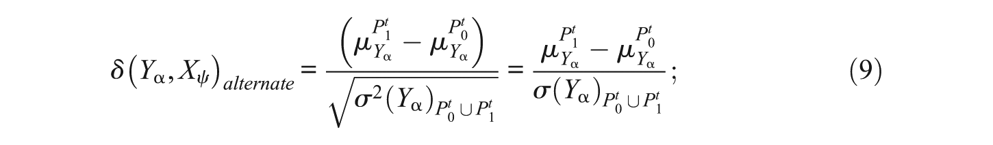
Let an alternate version of the population SMD, with the SD of scores in the population

where
Relationship Between Common and Alternate Versions of the SMD
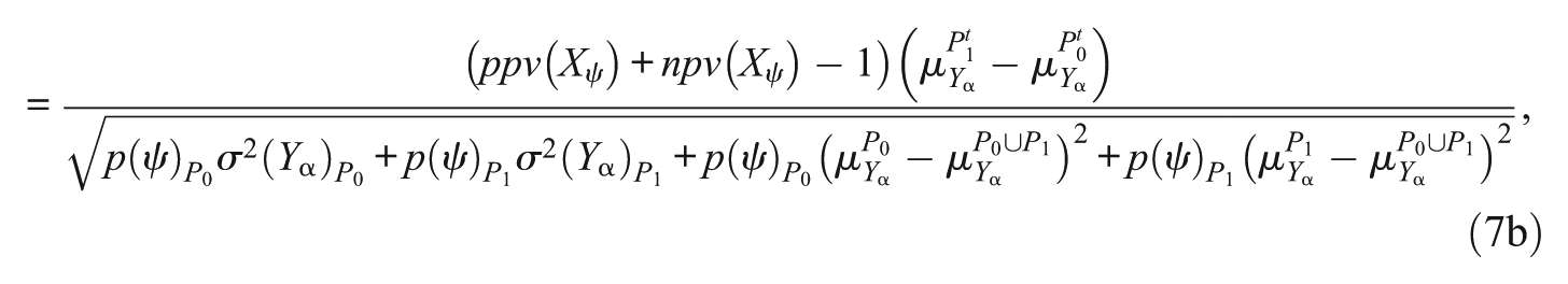
It is straightforward to show the relationship between the common and alternate versions of the SMD is given by Equation (8),
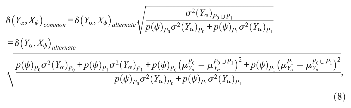
where
Figure 2 shows a plot of common and alternate SMDs as a function of the difference between the means of
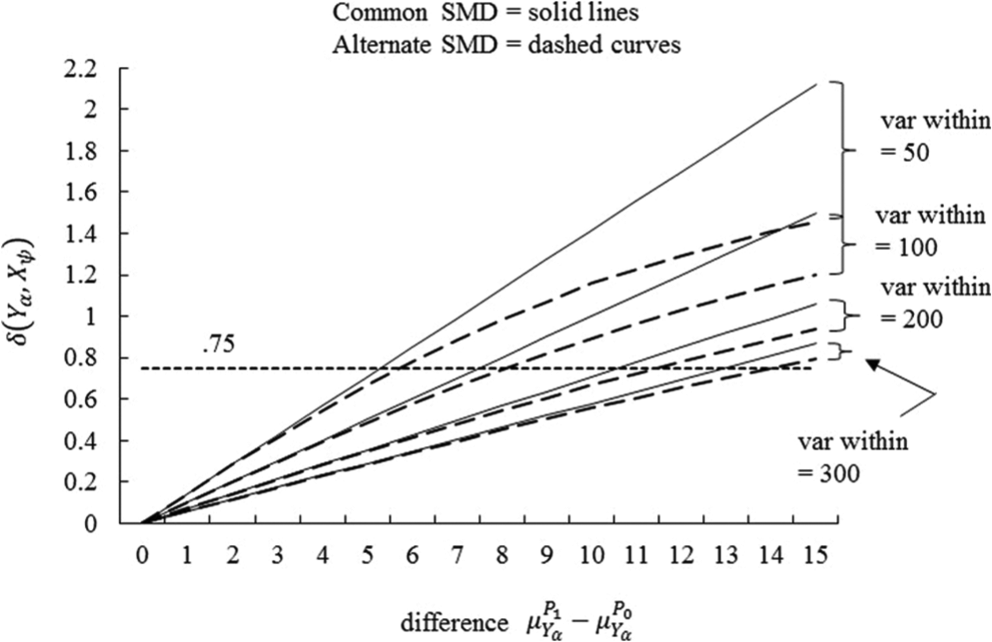
Graph of values of common (solid lines) and alternate (dashed curves) versions of the population SMD as a function of the between population mean difference,
The values of the two versions of the population SMD are nearly identical in this graph up to common SMD values of about .75 (marked by the dotted horizontal line), with differences between the two versions of .05 or less. The values differentially and increasingly diverge from this point, with the magnitude of the divergence a function of the magnitude of the within population variances; the smaller the mean within population variance, the greater the divergence. These differences between the two SMD versions are considered below.
The Effects of Measurement Error in the IV: A Simulation
A model-based simulation was conducted to investigate the magnitude by which the population common SMD is attenuated by measurement error in the IV. A model-based simulation uses a mathematical model to investigate the behavior of some real-world system or method under specified conditions (Axelrod, 2007; Banks, 2009; Harrison, Lin, Carrol, & Carley, 2007). In this simulation, the mathematical model was that of the common SMD expressed by Equations (3) through (6), and the method investigated was the representation of the difference between the means of populations
In the simulation, the absence of measurement error in the DV was assumed, and the “true” common SMD, defined as its value when there was no measurement error in either DV or IV, was +.50, a value equal to the mean common SMD found in the analysis of over 300 meta-analyses by Lipsey and Wilson (1993). The subpopulations
Figure 3 shows the error in the common SMD, with “error” defined as the difference between the common SMD affected by simulated measurement error in the IV and its “true” value of +.50, plotted as a function of measurement error in the IV for two prevalence rates: .50 and .09. The prevalence of .50 simulated experimentally created subpopulations of persons, one of which received a treatment and one that did not (solid curves). The prevalence of .09 simulated a low prevalence context, such as the 1-year prevalence of MDD in the United States (dashed curves). The error is represented on the vertical axis; measurement error in the IV as indicated by sensitivity is scaled on the horizontal axis, and as indicated by specificity, with values ranging from 1.0 to 0.40, marked for the curves. For example, the top solid curve shows the error as a function of sensitivity given the prevalence was 0.50 and
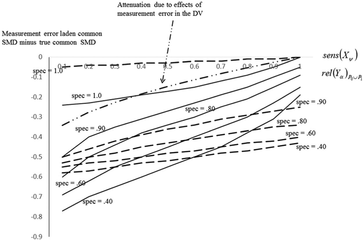
Graph showing the attenuation in the population common SMD due to differing levels of measurement error in the IV. The solid curves show the attenuation in the SMD given the prevalence of the characteristic differentiating membership in
As this graph shows, the error in the common SMD increases as measurement error in the IV increases; as either the sensitivity or specificity, or both, decrease from 1.0, the error increases. One way of assessing the practical significance of the errors is by comparing them with the SD, 0.29, of the distribution of mean common SMDs from Lipsey and Wilson (1993). For example, the error in the common SMD, given a prevalence of .50 and holding the sensitivity constant at 1.0, increased from 0 to −.09 as the specificity decreased from 1.0 to 0.80, a magnitude about .3 SD in the Lipsey and Wilson distribution. In contrast, given a prevalence of .09, the error in the SMD increased from 0 to about −.34, about 1.2 SD in the Lipsey and Wilson distribution, as the specificity decreased from 1.0 to 0.80 while holding the sensitivity constant at 1.0. Given a prevalence of .50, the error in the common SMD increased from 0 to −.21 as both sensitivity and specificity decreased from 1.0 to 0.80, an error covering .70 SD in the Lipsey and Wilson distribution. Given a prevalence of .09, the error in the SMD increased from 0 to −.37, about 1.3 SD in the Lipsey and Wilson distribution, as sensitivity and specificity both decreased from 1.0 to 0.80.
The errors in the common SMD in Figure 3 indicate attenuation, results consistent Hunter and Schmidt’s (2004) observations. These results also suggest the effects of measurement error in the IV on the common SMD are moderated by prevalence. A graph of errors in the numerator of the common SMD, similar to Figure 3 and omitted here in the interest of brevity, shows substantial attenuation in the numerator of the SMD as sensitivity and specificity decrease from 1.0. For example, given a prevalence of .09, the difference in the numerator decreased from 5.0 to 1.3 as both sensitivity and specificity decreased to .80. These results suggest the errors in the common SMD in Figure 3 are due prominently to the effects of measurement error in the IV on the numerator of the SMD.
Relative Effects of Measurement Error in IV and DV
The dash-dot-dot curve in Figure 3 shows error in the common SMD as a function of measurement error in the DV, assuming no measurement error in the IV. For this curve the horizontal axis is scaled as the reliability coefficient for scores from the DV in
A Proposed Method for Correcting the Common and Alternate Versions of the SMD for Measurement Error in the IV
Theoretical Rationale
Define the term
the alternate version of the SMD is completely reliability corrected for the effects of measurement error in the IV.
A Proposed Method for Reliability Correcting the SMD
The foregoing suggests the following method for disattenuating the numerator of the SMD, thereby partially reliability correcting the common SMD, and completely reliability correcting the alternate SMD, for the effects of measurement error in the IV.
Step 1
Obtain sample estimates of the means and variances of the DV in populations
Step 2
An estimate of the numerator disattenuated, partially reliability corrected common SMD, symbolized as

An estimate of the reliability corrected alternate SMD, symbolized as

Reliability Correcting the Unstandardized Mean Difference
Lipsey and Wilson (2001) defined the unstandardized mean difference (UMD) as

the UMD is the numerator of the population SMD. It follows as a corollary of the foregoing that the UMD can be disattenuated for the effects of measurement error in the IV from

Conceptual Interpretation of
Equations (6) and (7) imply the relationship between the difference

Thus,
The values of
Return to the Illustrative Example
Consider again the illustrative example from the introduction. The estimated common SMD was .187, and the Hunter and Schmidt method produced a reliability-corrected common SMD of .387. The alternate SMD would be, in this case, .185, nearly the same as the common SMD. In this example,
A Series of Monte Carlo Simulations
A series of Monte Carlo studies of the two reliability correction methods were conducted (Axelrod, 2007; Banks, 2009; Mooney, 1997). The objectives of these simulations were to (a) obtain Monte Carlo estimates of the sampling distributions of the numerator disattenuated, partially reliability corrected common, and reliability corrected alternate, SMDs obtained using both the proposed method and the Hunter and Schmidt (2004) approach; (b) compare these two methods in terms of bias, efficiency, and the ranges of estimates; and (c) investigate the extent to which disattenuating the numerator of the common SMD effectively reliability corrects it for the effects of measurement error in the IV. Bias was defined as the difference between the mean of the sampling distribution of the estimated reliability corrected SMD and the true value of the measurement error free population SMD. Efficiency was represented in terms of mean squared error (MSE; Taboga, 2012).
Methodology
Figure 1 helps in describing the methodology of these simulations. First, DV scores for populations
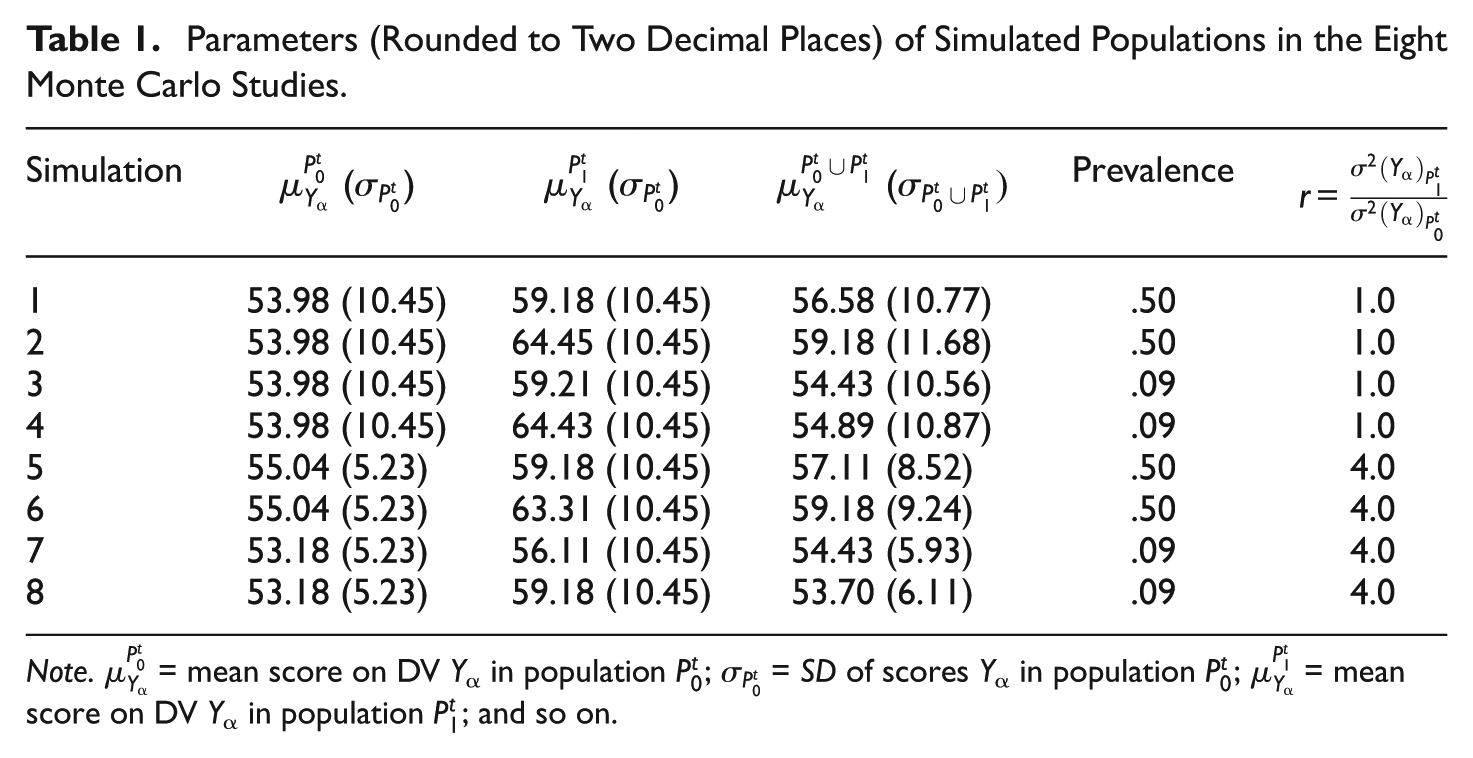
Parameters (Rounded to Two Decimal Places) of Simulated Populations in the Eight Monte Carlo Studies.
Note.
The classification of persons from
To investigate their possible effects on the reliability correction methods, three factors were varied in the simulations: prevalence of the characteristic of interest in
Finally, two values of the variance ratio, r, were simulated: 1.0, consistent with equal variances in populations
Simulation (1): prevalence = .50, r = 1, true common SMD = .50
Simulation (2): prevalence = .50, r = 1, true common SMD = 1.0
Simulation (3): prevalence = .09, r = 1, true common SMD = .50
Simulation (4): prevalence = .09, r = 1, true common SMD = 1.0
Simulation (5): prevalence = .50, r = 4, true common SMD = .50
Simulation (6): prevalence = .50, r = 4, true common SMD = 1.0
Simulation (7): prevalence = .09, r = 4, true common SMD = .50
Simulation (8): prevalence = .09, r = 4, and true common SMD = 1.0
Once populations

The reliability corrected common and alternate SMDs were estimated for each random sample using the methods described earlier, giving 6,000 estimates in each simulation. In those simulations in which the prevalence was .50,
Results
The results of the Monte Carlo simulations are shown in Table 2. The first column identifies the simulation number (1 to 8); the SMD being reliability corrected (
The means of the sampling distributions, with the differences between means of sampling distributions and true measurement error free SMDs (bias) in parentheses
The SDs of the sampling distributions
The ranges of estimates of the reliability corrected SMDs
99.9% confidence intervals (CIs) for bias in the estimates. The CIs for reliability corrected SMDs obtained using the proposed method were normal curve based, while those from the Hunter and Schmidt method were bootstrap CIs given these sampling distributions were nonnormally distributed. A 99.9% CI that included 0 was taken to indicate an unbiased estimate, and vice versa. Use of 99.9% CIs gave an overall type I error rate for bias inferences of less than .05 over the 32 CIs
MSE values
Kolmogorov–Smirnov Z-statistics for tests of normality of the sampling distributions
Results of Eight Monte Carlo Simulations.
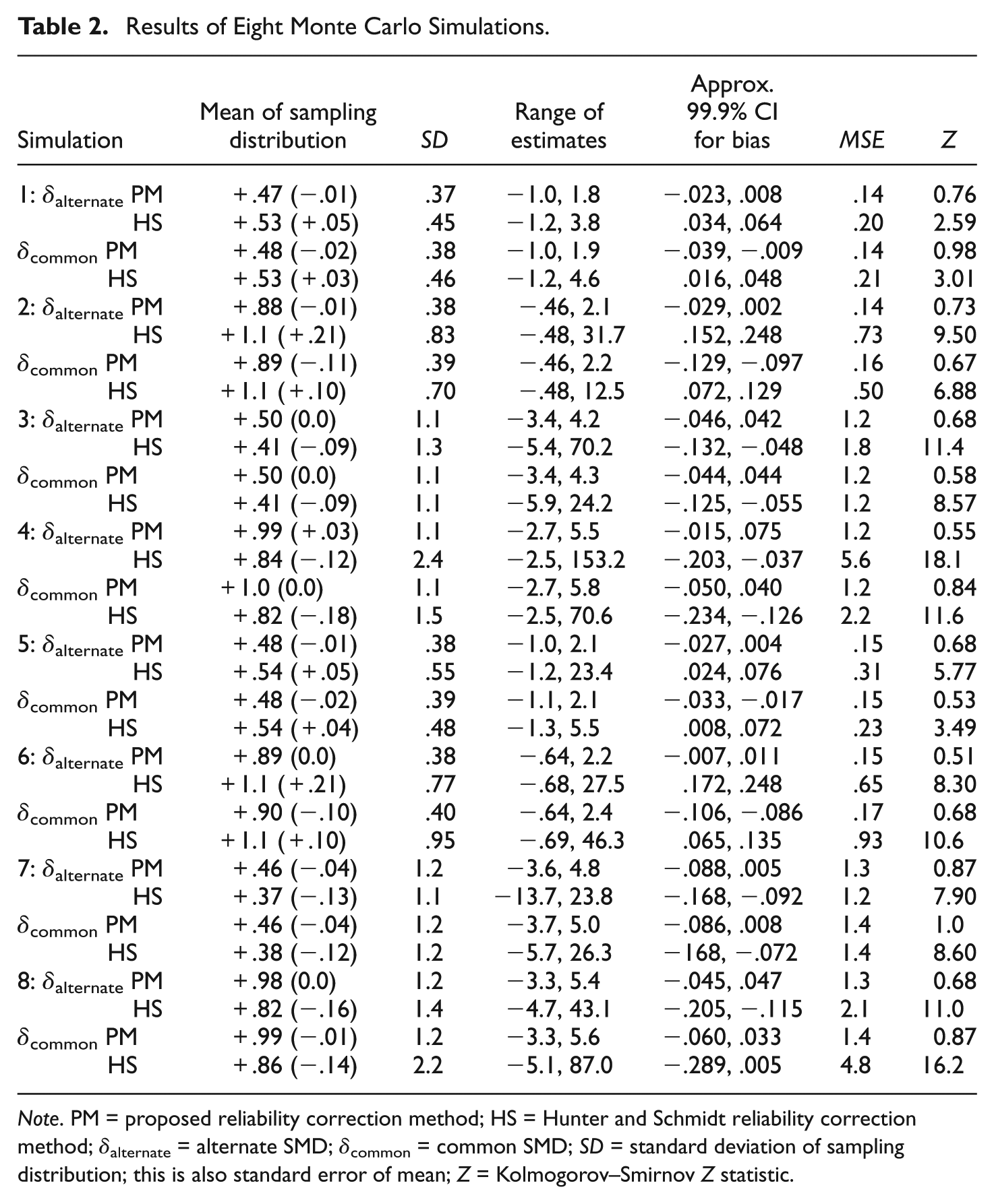
Note. PM = proposed reliability correction method; HS = Hunter and Schmidt reliability correction method; δalternate = alternate SMD; δcommon = common SMD; SD = standard deviation of sampling distribution; this is also standard error of mean; Z = Kolmogorov–Smirnov Z statistic.
Results Comparing Hunter and Schmidt and Proposed Methods
The proposed reliability correction method had lower bias values, controlling for version of SMD (alternate or common), prevalence, variance ratio (r), and magnitude of the measurement error free population SMD, than the Hunter and Schmidt approach, and the differences in bias were moderated by prevalence, F(1, 25) = 64.6, p < .001, with the moderating relationship uniquely accounting for about 48% of the variation in bias. 1 Given a prevalence of .50, the mean bias in estimated reliability corrected common SMDs using the Hunter and Schmidt (2004) method was about, .07 (95% CI: .02, .1); and given a prevalence of .09, about −.13 (95% CI: −.18, −.09). Given a prevalence of .50, the mean bias using the Hunter and Schmidt method to reliability correct the alternate version of the SMD was about .13 (95% CI: .08, .18); and given a prevalence of .09, about −.13 (99% CI: −.17, −.08).
In contrast, given a prevalence of .50, the mean bias in estimates of the reliability corrected common SMD using the proposed method to disattenuate the numerator was −.06 (95% CI: −.11, −.02); and given a prevalence of .09, −.01 (95% CI: −.06, .04). Given a prevalence of .50, the mean bias in estimated reliability corrected alternate SMDs using the proposed method was −.008 (95% CI: −.06, .04); and given a prevalence of .09, −.003 (95% CI: −.05, .05).
The proposed method was overall more efficient than the Hunter and Schmidt (2004) method in terms of MSE. Controlling for version of the SMD, prevalence, variance ratio, and magnitude of the measurement error free SMD, the difference between the MSE for Hunter and Schmidt (2004) estimated reliability corrected SMDs and that for estimates from the proposed method was .79, F(1, 26) = 6.93, p < .05 (95% bootstrap CI for difference: .11 to 1.5). 2 The MSE of estimates of the reliability corrected SMDs was also strongly associated with prevalence, controlling for the other factors in the simulations, F(1, 26) = 28.2, p < .001, unique R2 = .425. The difference between the mean MSE associated with estimated reliability corrected SMDs for a prevalence of .09 and that for a prevalence of .50, controlling for the factors in the simulation, was about 1.6 (95% bootstrap CI for difference: .9 to 2.3). Estimates in the higher prevalence context were overall more efficient. There was also evidence suggesting the proposed method produced more efficient estimates in the .09 prevalence context, mean MSE = 1.28, than the Hunter and Schmidt method, mean MSE = 2.54 (95% bootstrap CI for difference: .42 to 2.1).
The proposed method also produced, overall, estimates with narrower ranges of estimates, and lower extreme values, regardless of whether the reliability correction was for the common or alternate SMD. The mean range of estimates for the proposed method was from −2.0 to about 3.4; and for the Hunter and Schmidt method, −3.3 to 40.8.
Summary of Results
The proposed method appeared superior to the Hunter and Schmidt approach in terms of producing unbiased estimates of both common and alternate SMDs disattenuated for the effects of measurement error in the IV in the .09 prevalence context. The proposed method produced estimates of the reliability corrected common SMD with a downward mean bias of about .06 given a prevalence of .50. The proposed approach produced overall more efficient estimates, in terms of MSE, of reliability corrected SMDs than the Hunter and Schmidt method.
The Illustrative Example: Conclusion
The illustrative example, considered earlier at two points in this article, comes from a simulation in which the population parameters were
Conclusion
The results of the simulation in Figure 2 suggest attenuation in the SMD due to measurement error in the IV depends on prevalence, can be particularly pronounced when prevalence is low, and can exceed that due to measurement error in the DV. The results also suggest significant attenuation can occur at levels of measurement error, as indicated by sensitivity and specificity values, found in scores from measures currently used. In the illustrative example, the sensitivity and specificity values were .717 and .90, respectively, mean values from a recent review of interview methods used to identify persons with MDD. The measurement error implied by these values, in context of the MDD prevalence in the United States of about .09, led to an attenuation factor of .385; the magnitude of the SMD numerator, common or alternate, would be slightly more than one-third its value were there no measurement error in the IV. These findings imply significant attenuation due to measurement error in the IV may exist in SMDs reported in research, especially in low prevalence population comparison studies.
Given that levels of measurement error in the IV may vary across studies, the degree of attenuation in SMDs will vary across studies. As noted earlier, this differential attenuation will propagate through meta-analyses, a problem likely compounded by differential measurement error in DVs. The propagation of differential attenuation of SMDs through meta-analyses can potentially lead to erroneous results and conclusions. The proposed reliability correction method appears a promising approach for disattenuating the SMD, common or alternate, due to measurement error in the IV, thereby increasing the validity of results from meta-analyses.
The results of the Monte Carlo simulations support use of the proposed method of correcting the alternate version of the population SMD for the effects of measurement error in the IV, regardless of prevalence. The results support its use for reliability correcting the common SMD, especially in lower prevalence contexts, by disattenuating the numerator of the SMD for the effects of measurement error in the IV. The proposed method appears most promising for disattenuating SMDs from population comparison studies. The proposed reliability correction method could be implemented in a meta-analysis in a manner analogous to that suggested by Hedges and Olkin (1985) for meta-analyzing SMDs corrected for measurement error in the DV. The weighted reliability corrected estimate of the SMD would be given by formula (40); confidence intervals by formulas (41) and (42); and a test of homogeneity of SMDs corrected for measurement error in the IV using formula (43) in Lipsey and Wilson (2001), but with the term
As currently formulated the proposed method is based on the assumption persons in
The proposed reliability correction method needs further theoretical development to be applicable in measurement scenarios such as that immediately above. One approach to generalizing the reliability correction method developed above might be to derive expressions for the sensitivity and specificity conditional on values of the observed scores from the measure of the IV. These might be based, for example, on a receiver operating characteristic curve for the relationship between the scores on the IV measure and classification (Pepe, 2003; Swets, 1988). The expressions for these conditional sensitivity and specificity values could then be used to derive expressions for the conditional PPV and conditional NPV. From these a disattenuation factor similar to
The proposed reliability correction method, like the method sketched by Hunter and Schmidt (2004), can only be used to correct for the effects of random measurement error in the IV. It will not correct for systematic error. Hunter and Schmidt (2004) discussed systematic measurement error under the conceptual umbrella “imperfect construct validity.” In this exposition, Hunter and Schmidt considered three approaches to dealing with systematic error in the IV. The reader is referred to this source for in depth consideration of this issue in meta-analysis.
The graph of common and alternate versions of the SMD in Figure 2 suggests the difference between the two versions will be .05 or less for common SMD values of about .75 or lower. This implies the alternate version of the SMD might be used in circumstances in which the common SMD would be .75 or less, and Lipsey and Wilson’s (1993) findings suggest this may occur rather frequently, with relatively minimal differences between the two versions of the SMD. Earlier it was argued a principal advantage of use of the alternate SMD is the insensitivity of the denominator to the effects of measurement error in the IV, and the ability to correct this version of the SMD for the effects of measurement error in the IV by dividing it by
Recent work has been done on the development of regression coefficient based EFSs for use in meta-analysis (e.g., Kim, 2011). An interesting line of future research and theoretical development is investigation of the extension of the proposed reliability correction method to correcting regression-based EFSs for the effects of measurement error in the IV. Keef and Roberts’ (2004) recently proposed “partial standardized mean difference” appears to be an interesting regression based EFS on which to focus. The partial SMD is, essentially, a SMD that has been adjusted for a covariate. Generalization of the proposed reliability correction method to this particular regression based EFS might open the door to application of the method to other regression based EFSs, such as those developed by Kim (2011). It might also provide a link between reliability correcting meta-analytic EFSs and correcting regression coefficients for the effects of measurement error in the IV.
Finally, the results of the Monte Carlo simulations have implications for future research. Monte Carlo simulations investigating the use of the proposed reliability correction method with both the common and alternate SMDs need to be done with prevalence values different from those in the current simulations. Prevalence rates lower than .09; between .09 and .50; and above .50 need to be done. The bias and efficiency of the two reliability correction methods needs to be investigated as a function of these prevalence rates. The results of the current simulations suggest the hypothesis that the proposed method used to reliability correct the alternate version of the SMD will produce unbiased estimates regardless of prevalence. A specific research question concerns the prevalence at which disattenuation of the numerator of the common SMD using the proposed reliability correction method ceases to give unbiased estimates of the common SMD corrected for the effects of measurement error in the IV. The results of the current simulations imply this point will be in the neighborhood of .50. The results of the Monte Carlo simulations also suggest the Hunter and Schmidt method might produce unbiased estimates at some prevalence rates between .09 and .50. Factors other than those studied in the current Monte Carlo studies need to be varied in future simulation studies of the proposed method, such as sample size.
Footnotes
Appendix
Declaration of Conflicting Interests
The author(s) declared no potential conflicts of interest with respect to the research, authorship, and/or publication of this article.
Funding
The author(s) received no financial support for the research, authorship, and/or publication of this article.