Is the Factor Observed in Investigations on the Item-Position Effect Actually the Difficulty Factor?

Abstract

In confirmatory factor analysis quite similar models of measurement serve the detection of the difficulty factor and the factor due to the item-position effect. The item-position effect refers to the increasing dependency among the responses to successively presented items of a test whereas the difficulty factor is ascribed to the wide range of item difficulties. The similarity of the models of measurement hampers the dissociation of these factors. Since the item-position effect should theoretically be independent of the item difficulties, the statistical ex post manipulation of the difficulties should enable the discrimination of the two types of factors. This method was investigated in two studies. In the first study, Advanced Progressive Matrices (APM) data of 300 participants were investigated. As expected, the factor thought to be due to the item-position effect was observed. In the second study, using data simulated to show the major characteristics of the APM data, the wide range of items with various difficulties was set to zero to reduce the likelihood of detecting the difficulty factor. Despite this reduction, however, the factor now identified as item-position factor, was observed in virtually all simulated datasets.

Keywords

difficulty factor item difficulty item-position effect method effect

An additional factor observed in the investigation of the structural validity of a scale is not necessarily the item-position factor. Even if this factor is expected, the additional factor may in fact be the difficulty factor instead of the item-position factor. One way of making sure that the additional factor is the item-position factor is to rule out that it is the difficulty factor that is the major alternative to the other factor. This indirect way of identifying the item-position factor is possible because the observation of the difficulty factor depends on the configuration of the difficulties of the items. The following sections outline a method of making use of this dependency for identifying the item-position factor. Furthermore, the usefulness of this method is demonstrated in an application including an empirical and a simulation study.

The item-position effect refers to the increasing dependency of the response to an item on the position of this item within a series of test items; it gradually develops during test taking from the first to the last item of a scale. Item homogeneity and a broad range of item difficulties are the main characteristics of scales reported to show the item-position effect. The item-position effect was primarily found in homogeneous intelligence scales such as Raven’s Advanced Progressive Matrices (APM; Raven, Raven, & Court, 1997). Other denotations of the item-position effect or closely related effects are contextual effect, item-order effect, serial-position effect, item-context effect, practice effect, and serial dependency (e.g., Vogt, 2005). The most convincing explanation presented so far asserts that learning during test taking is the main source of the item-position effect (Carlstedt, Gustafsson, & Ullstadius, 2000; Embretson, 1991; Verguts & De Boeck, 2000). According to this assertion, the item-position effect is not a simple bias but an additional and potentially valuable source of information.

Studies by Campbell and Mohr (1950) and Mollenkopf (1950) were presumably the first reports on the item-position effect. Initially there were a number of experimental studies on the topic (e.g., Knowles, 1988; Knowles & Byers, 1996). Later on this effect was also identified by means of item response theory (IRT) techniques (e.g., Debeer & Janssen, 2013; Embretson, 1991; Gittler & Wild, 1989; Verguts & De Boeck, 2000) and in the framework of confirmatory factor analysis (CFA; e.g., Hartig, Hölzel, & Moosbrugger, 2007; Schweizer, 2012; Schweizer, Schreiner, & Gold, 2009). While IRT techniques examine the change of response probabilities due to the item-position effect, investigations using CFA concentrate on the interindividual variability in the responses to the test items. Selecting the CFA framework, as done in the present article, means that the focus is on the systematically increasing variance from the first to the last item. In CFA, the item-position effect is represented by a factor that complements another factor representing the construct, that is, the content factor.

This CFA-based way of investigating the item-position effect shares characteristics with other CFA-based ways of addressing concerns regarding the validity of psychological scales. First there is the multitrait–multimethod approach that also assumes that there is a second systematic source of responding besides the main source (Kenny & Kashy, 1992; Marsh, 1989; Marsh & Bailey, 1991; Widaman, 1985). In this case, the other source is assumed to originate from the employed observational method in general. Second, there is the research into the item wording effect. Equal numbers of positively and negatively worded items appear to impair model fit considerably whereas items of the same wording do not (DiStefano & Motl, 2006; Vautier, Steyer, Jmel, & Raufaste, 2005).

There is a complication, however, that has so far not been considered appropriately in the factor-analytic research on the item-position effect: The broad range of item difficulties characterizing the intelligence scales found to show the item-position effect is also considered as the source of the so-called difficulty factor (Ferguson, 1941; Gibson, 1960; McDonald & Ahlawat, 1974). This factor is ascribed to the wide range of items with various difficulties whereas the arrangement of the items within this range does not count. Furthermore, it seems that close similarity of some binary items according to difficulty within the wide range of items drives the observation of the difficulty factor additionally (Bandalos & Gerstner, 2016). Moreover, the binary nature of items is considered as another precondition of the difficulty factor (Floyd & Widaman, 1995). In order to suppress the difficulty factor Kishton and Widaman (1994) suggest the computation of item parcels. Another way of dealing with the difficulty factor is to explicitly depict it in terms of nonlinear models of measurement and nonlinear factor analysis (McDonald, 1965; McDonald & Ahlawat, 1974). This essay adds another possibility of identifying the difficulty factor as such a factor.

Despite extensive research on the difficulty factor, so far no other source of this factor has been detected than the wide range of items with various difficulties. Therefore, it is considered as a method bias with no further implications for substantive research. The emphasis on the wide range of items with various difficulties suggests that the difficulty factor depends on spuriously high correlations between very easy or between very difficult items. Such correlations create local homogeneity, which cannot be accounted for by the content factor (Bandalos & Gerstner, 2016).

A major precondition for the emergence of the item-position effect and the difficulty factor is the combination of binary items and a broad range of item difficulties. However, there are also differences: first, the factor representing the item-position effect is not restricted to binary data (see, e.g., Hartig et al., 2007) whereas the difficulty factor is. Second, there are differences regarding the source of the additional factor. With respect to the difficulty factor the model of measurement proposed by McDonald and Ahlawat (1974) suggests that the content and additional factors grow out of the same source. This is obvious from the use of the same random variable as argument for representing these two factors whereas the item-position effect is clearly ascribed to an extra source (Carlstedt et al., 2000; Embretson, 1991; Verguts & De Boeck, 2000). Third, the descriptions of the properties of the data leading to the difficulty factor suggest that this factor is due to coincidences of values at random amplified by specific constellations of items whereas the item-position factor appears to represent a cognitive source (Ren, Goldhammer, Moosbrugger, & Schweizer, 2012).

The investigations reported in the following sections proceed from the assumption that the factor representing the item-position effect, henceforth referred to as item-position factor, is not identical with the difficulty factor. Proceeding from this assumption, we aimed to dissociate the item-position factor from item difficulty factor. Since the wide range of items with various difficulties is essential for observing the difficulty factor but not for the item-position factor, manipulating the range of item difficulties seems to be a feasible method to dissociate the two factors. More specifically, diminishing the range of item difficulties should weaken the difficulty factor but not influence the item-position factor. The other possible ways of dealing with the difficulty factor, nonlinear factor analysis (McDonald, 1965; McDonald & Ahlawat, 1974) and computing item parcels (Kishton & Widaman, 1994), are not suitable for this purpose. Nonlinear factors are too specific und nowadays treated as genuine factors whereas item parcels can be expected to impair the item-position effect besides suppressing the difficulty factor.

The Separation of the Two Effects

Reducing the broad range of item difficulties to zero by setting all item difficulties to the same size, referred to as zero range, is the way selected for the separation of the two factors in the present study. Setting the difficulties of all items to the same value in all positions of a sequence of items should suppress the difficulty factor whereas the item-position factor should remain unaffected. For this purpose, the method outlined in this section adapts a procedure employed in the generation of data for simulation studies (Jöreskog & Sörbom, 2001).

Assume the n×p matrix M_broad-binary comprising the binary outcomes {0, 1} of n participants completing the p items of an intelligence scale that show a broad range of item difficulty. Despite the binary nature of the responses, it is commonly assumed that the participants’ true attributes underlying each response are continuous and stem from a normal distribution. The numerical description of these attributes is assumed to be given by the n×p matrix M_{latent-continuous}. Equation (1) provides a formal description of how measurement by the set of p items abbreviated as dichot_{broad-range measurement} leads to the available data:

M_{broad - binary} = {dicho t}_{broad - range measurement} (M_{latent - continuous}) .

(1)

In order to achieve data that cannot give rise to a difficulty factor, the intelligence test data must be transformed in an ex post operation in such a way that they show the zero range of item difficulties. The hypothetical function for arriving at the zero range is abbreviated as dichot_{zero-range measurement}. Applying this function leads to the n×p matrix M_zero-binary:

M_{zero - binary} = dicho t_{zero - range measurement} (M_{latent - continuous}) .

(2)

As indicated above, M_zero-binary can be obtained in a simulation study. A major prerequisite of such a study is a relational pattern that reflects the covariances of the columns of M_{latent-continuous}. These covariances are included in the p×p matrix S(M_{latent-continuous}) that is unknown because M_{latent-continuous} is unknown. If an estimate of this covariance matrix is available, the procedure described by Jöreskog and Sörbom (2001) can be used for generating matrices of simulated data that are estimates of M_{latent-continuous}. Subsequently, each estimated matrix ${\hat{M}}_{latent - continuous}$ can be statistically transformed into both ${\hat{M}}_{broad - binary}$ and ${\hat{M}}_{zero - binary}$ .

To underscore the reasoning at this point, the result of a simulation study is reported. Assuming a uniform relational pattern including .30 as value of the off-diagonal elements and 1.00 as value of the diagonal elements, five hundred 500×15 matrices of continuous data were generated and dichotomized. The dichotomization of the data included in the columns of the matrices yielded binary data. The dichotomization was conducted in four different ways: (1) to achieve a zero range of item difficulties, the numbers included in the columns of a matrix of continuous data were split even into zeros and ones; (2) to arrive at a broad range of item difficulties, the 15 hypothetical probabilities of a correct response associated with the columns were varied with equal distances between .1 and .9 and used to split the numbers of the columns; (3) for having a broad range of 13 item difficulties with equal distances among each other and two more item difficulties that corresponded to two of the other item difficulties to give two pairs of items showing the same item difficulty, the corresponding probabilities were used for splitting the numbers of the columns; and (4) in order to have a broad range of 11 different item difficulties with equal distances among each other and four more item difficulties giving rise to two triplets with one of two other item difficulties, the columns were split according to the corresponding probabilities. Note. When referring to matrices the term probability is preferred over the term item difficulty; these probabilities are assumed to reflect item difficulties. Figure 1 provides the percentages of observing an additional factor that is a difficulty factor since there is no other source for the additional factor.

Figure 1.

Percentages of detections of a difficulty factors in comparing the fit results of one- and two-factor models in 500 datasets when the range of item difficulty was zero, broad, broad and including two pairs of items showing the same item difficulty and broad and including two triplets of items showing the same item difficulty.

As is obvious from the sizes of the bars, in the zero range of item difficulties the percentage of difficulty factors is negligible, in the broad range there is a considerable increase of the percentage, and the inclusion of subsets of items showing the same item difficulty causes additional sizable increases. Although it is our experience that there can be rare circumstances giving rise to larger percentages, it should be noted that it is more likely to observe no difficulty factor than detecting one.

Because of the great importance of the unknown S_{latent-continuous} [=S(M_{latent-continuous})] for the method of modifying the range of item difficulties, an evaluation of the appropriateness of the estimate that is used as replacement for the unknown relational pattern is necessary. For this purpose, the Euclidean distance is computed between the observed p×p covariance matrix S(M_broad-binary) and the mean of the set of simulated p×p covariance matrices $\bar{S ()}$ . Whereas S(M_broad-binary) is obtained from M_broad-binary, $\bar{S ()}$ is computed from the simulated data using the splits according to the original items. The Euclidean distance is then compared with a preset criterion c_broad-binary:

c_{broad - binary} > ‖ S (M_{broad - binary}) - \bar{S ({\hat{M}}_{broad - binary})} ‖ .

(3)

The value of c_broad-binary must be selected by the researcher according to the necessary degree of precision.

The Estimation of the Relational Pattern

This section outlines a possible way to obtain an estimate of S_{latent-continuous} that can be used as replacement for the unknown relational pattern. This way is designed to reverse the transformations inherent in the dichotomization of originally continuous data. The reversion concentrates on the distortions of the variances and covariances of the observed p×p covariance matrix S(M_broad-binary) due to dichotomization. The first step concentrates on the reversal of the deviations of the variances from the expected variances due to the skewness of the data distributions whereas the second and third steps serve the correction for attenuation due to dichotomization (Schweizer, 2013; Schweizer, Ren, & Wang, 2015). The first step is achieved by weighting the p columns of the data matrix. Each weight w_Ni (i = 1, . . ., p) that includes the subscript N to indicate the implicit aim that is similarity to normality is defined as the function of the probability that item X_i (i = 1, . . ., p) is answered correctly:

w_{N i} = \sqrt{\frac{0.25}{\Pr (X_{i} = 1) [1 - \Pr (X_{i} = 1)]}}

(4)

where Pr(X_i = 1) with 0 < Pr(X_i = 1) < 1 is the probability of a correct response with respect to item X_i. The other steps are supposed to reverse the general effect of dichotomization known as attenuation. The second step requires the multiplication of all coefficients of the observed covariance matrix by four. As a consequence of the first and second steps, all numbers of the main diagonal are one. For ease in notation the weights w_Ni (i = 1, . . ., p) of the first step and the square root of the multiplier of the second step $\sqrt{4}$ are combined to give the elements of the main diagonal of the p×p diagonal matrix W_N.

However, there is a complication due to the concomitant change of the relative contributions of the true and error variances to the observed variances of the items. This is obvious from the rule regarding the summation of variances. The variance of the sum of the random variables X_i and X_j with the variances var(X_i) and var(X_j) is given by

var (X_{i} + X_{j}) = var (X_{i}) + var (X_{j}) + 2 cov (X_{i}, X_{j}) .

(5)

After replacing cov(X_i, X_j) by the product of the correlation r of X_i and X_j and the standard deviations of the random variables, the type of data can be taken into consideration. If X_i and X_j represent true scores, r = 1. In contrast, if X_i and X_j represent error, r = 0. This means that the true part of the variance increases more than the error part of the variance when the composite variance increases. While in the second step the variances of the items increase from 0.25 to 1.00 the relative amounts of the true and error parts change additionally. This change also affects the covariances that do not include error according to the model of the covariance matrix. As a consequence, they increase more than the variances of the items. Therefore, it is proposed to estimate the parameter v_C that is assumed to reflect the disproportional increase of the covariances. The estimation of this parameter requires the minimization of the following Euclidean distance:

min ‖ {S (M_{broad - binary}) - diag [S (M_{broad - binary})]} - {\bar{S ({\hat{M}}_{broad - binary})} - diag [\bar{S ({\hat{M}}_{broad - binary})}]} ‖

(6)

between the off-diagonal elements of the observed and simulated covariance matrices. Since v_C applies to all off-diagonal elements of the covariance matrices, it is included in the main diagonal of the p×p diagonal matrix V_C (v_Cii = v_Cjj) (i, j = 1, . . ., p). Finally, the matrices W_N and V_C are used for obtaining an estimate of S(M_{latent-continuous}):

\begin{matrix} \hat{S} (M_{latent - continuous}) = & W_{N} [diag S (M_{broad - binary})] W'_{N} + V_{C} {W_{N} [S (M_{broad - binary})] W'_{N}} V'_{C} - - V_{C} {W_{N} [diag S (M_{broad - binary})] W'_{N}} V'_{C} . \end{matrix}

(7)

The first summand of the mathematical expression to the right of the equality sign provides the main diagonal of the estimate of the relational pattern and the difference between the second and third summands the off-diagonal parts. The covariance matrix obtained this way refers to standardized data following the normal distribution and, therefore, can be used as replacement for the generation of continuous and standard normally distributed data.

Before closing this section, it needs to be emphasized that a major advantage of this method is that no assumption regarding the factor structure is imposed on the data. The simulated data computed in using the covariance matrix as relational pattern, or replacement of it, are not biased in favor of a specific structure, as is the normal case in simulation studies.

The Model for Investigating the Item-Position Effect

The confirmatory factor model for investigating data suspected to show the item-position effect must consider two latent sources of responding: (1) the basic ability that is represented by the items and thought to contribute to the response independently of the item position and (2) the source that gradually increases its contribution as a function of the item position. Whereas the basic ability is assumed to be a constant source, the contribution of the other source gradually unfolds from the beginning of the sequence of items to the end. The following equation provides the general model of measurement of CFA that needs to be adapted to the two sources:

Y = ν + Λ η + ε

(8)

where $Y$ is the p×1 vector of observations, $ν$ the p×1 vector of intercepts, Λ the p×q matrix of factor loadings, $η$ the q×1 vector of latent variables (i.e., factors) and $ε$ the p×1 vector of error components.

The adaptation of the general model to the two sources requires the constraint of the factor loadings since the free factor loadings of the standard CFA model (Jöreskog, 1971) tend to accommodate all kinds of deviations from expectations and this way “swallow” all kinds of effects. Constraining factor loadings means fixing the discriminability of the items (Lucke, 2005). Constrained discriminability also characterizes the Rasch model (1960) and the tau-equivalent model (Lord & Novick, 1968). Models with constrained factor loadings perform well if they correspond to the underlying structure of the data; otherwise they are likely to fail (Schweizer, Ren, Wang, & Zeller, 2015).

Knowles’s (1988) observation of increasing item reliabilities that are actually position reliabilities suggests that the item-position effect pertains to the true variances and covariances of the items. The factor loadings play a key role in the representation of the true variances and covariances in the model of the p×p covariance matrix Σ (Jöreskog, 1970):

Σ = Λ Φ Λ^{'} + Θ

(9)

where Λ is the p×q matrix of factor loadings, Φ the q×q matrix of the variances and covariances of the latent variables and $Θ$ the p×p diagonal matrix of error variances. The true variances of the items are represented by the diagonal elements of the product composed of ΛΦ and Λ′.

Since only Λ relates the items to the latent variables, the expected increase from one item to the next item must be represented by means of this matrix that includes two columns, one for basic ability and the other one for the item-position effect:

Λ = [{[\begin{matrix} λ_{11} \\ λ_{21} \\ . \\ . \\ λ_{p 1} \end{matrix}]}_{basic ability} {[\begin{matrix} λ_{12} \\ λ_{22} \\ . \\ . \\ λ_{p 2} \end{matrix}]}_{item - position effect}]

(10)

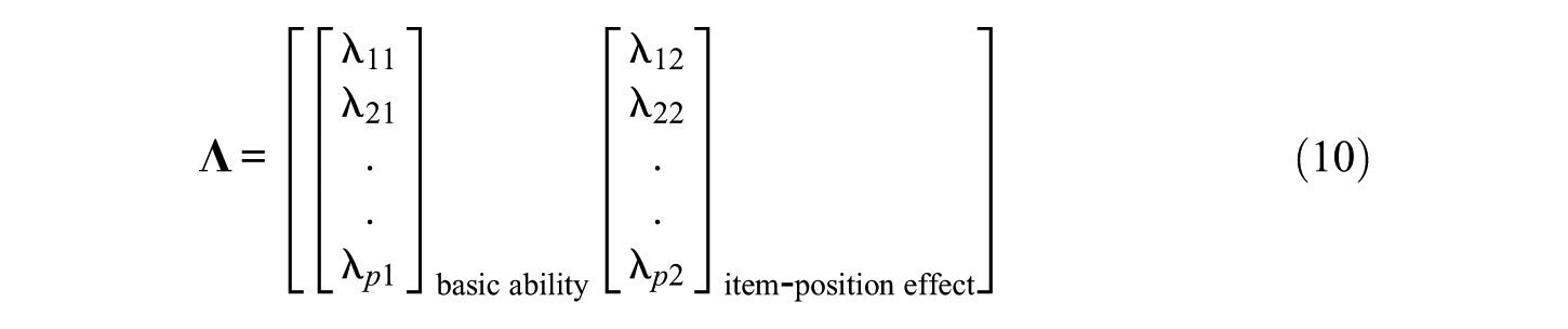
Since the source denoted basic ability is assumed to contribute to all responses equally, the number c (c>0) serves as constraint for all factor loadings of the first column. The constraints representing the item-position effect must show an increasing size. In this study the linear increase is preferred over other increases since the virtually linear increase of the item reliabilities of Knowles’ (1988) seminal study suggests a corresponding increase in the proportion of true variance. Furthermore, this increase agrees with the simplicity principle known as Occam’s razor. The described characteristics lead to the following matrix of factor loadings Λ that is identified as Λ_IPE:

Λ_{IPE} = [{[\begin{matrix} c \\ c \\ . \\ . \\ c \end{matrix}]}_{basic ability} {[\begin{matrix} 0 \\ 1 / (p - 1) \\ . \\ . \\ (p - 1) / (p - 1) \end{matrix}]}_{item - position effect}]

(11)

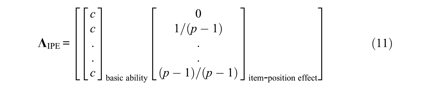
The numerator of the second column assures that the largest number is always one.

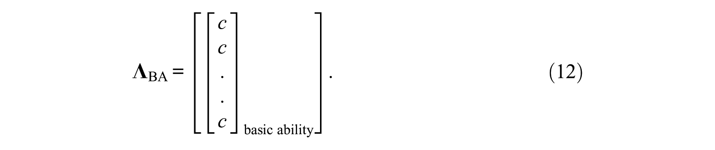
The identification of the item-position effect does not only require the demonstration of a good model–data fit but also the demonstration that the factor representing the item-position effect improves the model–data fit substantially. Such a demonstration can be accomplished by the comparison of the fit results for the model including a matrix of factor loadings according to Equation (11) with the fit results of another model that does not include a representation of the item-position effect. The matrix of constrained factor loadings Λ_BA of such a model is defined as follows:

Λ_{BA} = [{[\begin{matrix} c \\ c \\ . \\ . \\ c \end{matrix}]}_{basic ability}] .

(12)

Objectives

The major objective of this study was to check the nature of the additional latent variable (= factor) that was repeatedly observed besides the main latent variable in investigating intelligence scales. Based on empirical finding and theory either the item-position factor (= item-position latent variable) or the difficulty factor (= difficulty latent variable) was expected. It required to dissociate the item-position effect and the effect due to a wide range of items with various difficulties and thus to find out which kind of effect was the source of the additional latent variable. For this purpose, the presence of the additional latent variable was examined in the first Study that was an empirical study based on a sample of 300 participants who completed APM. Since the items of APM show a broad range of item difficulties, the observed effect might also be explained in terms of the difficulty factor. To rule out this explanation, we conducted a simulation study (Study 2) based on data constructed according to the covariance pattern of Study 1. In the core study design of this simulation, the variation of item difficulties was suppressed leading to the zero range of item difficulties. In case that the additional factor would disappear in the simulated data, it could be concluded that the additional factor of the first Study was a difficulty factor; otherwise it would be considered as the representation of the item-difficulty effect, that is, an item-position factor.

In order to increase the power of the second study, the described core study design was extended to a 2×2 factorial study design that included the following two main design factors: the design factors associated with the item-position effect and with the effect originating from the item difficulties. The design factor associated with the item-position effect was to be realized by using data simulated according the empirical pattern of the first study on one hand and by using data simulated according to a corresponding uniform pattern on the other hand. Whereas data simulated according to the empirical pattern of the first study could potentially be expected to give rise to the item-position factor, data simulated according to a corresponding uniform pattern could not. The second design factor included the following two conditions: data simulated to show the wide range of item difficulty and data simulated to have the zero range. The wide range was expected to lead to detections of the difficulty factor whereas the zero range was not.

Study 1: The Item-Position Effect in Advanced Progressive Matrices

The objectives of this research work required empirical data that could be demonstrated to include the item-position effect in Study 1 and could provide the relational pattern for data simulation in Study 2. APM data of 300 university students were available for this purpose. The reason for selecting APM data was that matrices problems were repeatedly shown to include the item-position effect (e.g., Kubinger, Formann, & Farkas, 1991; Lozano, 2015).

Method

Raven’s APM-Set II was composed of 36 items. The first six items were excluded because their probabilities of a correct response were virtually one that was too high to allow for a sizable item-position effect. The remaining items were subdivided into the subsets of 15 odd and 15 even numbered items in order to achieve an easily manageable size and to select the most suitable subset for the study. The criteria for the selection were (1) the range of item difficulties should be very broad and (2) the item difficulties should monotonically increase from the first to last items. Fortunately, one of the two subsets, the one composed of even numbered items, showed a good degree of agreement with both criteria.

Two CFA models were designed for this study. The first model included one latent variable with the factor loadings constrained according to Equation (12). In this model, the latent variable represented the basic ability which the scale was expected to represent. In the second model, there were two latent variables with the factor loadings constrained according to Equation (11). Thus, the basic ability and, additionally, the source of the item-position effect were assumed as latent factors in this second model. Because of the binary nature of the data, a link function applying to variances and covariances was additionally integrated into the model (Schweizer, Ren, & Wang, 2015).

The parameter estimation was conducted by means of the maximum likelihood estimation method using LISREL (Jöreskog & Sörbom, 2006). The following fit statistics were used for evaluating model-data fit: chi square, degree of freedom, normed chi square, root mean square error of approximatiom (RMSEA), standardized root mean square residual (SRMR), comparative fit index (CFI), Tucker–Lewis index (TLI), goodness-of-fit index (GFI), and Akaike information criterion (AIC). Cutoffs provided by Kline (2005) and Hu and Bentler (1999) served the evaluation of the results (normed χ² = 2, RMSEA = .06, SRMR = .08, CFI = .95, TLI = .95, GFI = .90; see also DiStefano, 2016). The comparisons between the models were conducted by means of the CFI difference (see Chen, 2007; Cheung & Rensvold, 2002) and the AICs for the models.

Results

The model with one latent variable yielded the following fit results: χ²(104) = 168.59, normed χ² = 1.62, RMSEA = .046, SRMR = .069, CFI = .87, TLI = .87, GFI = .93, and AIC = 200.59. The results for the model with two latent variables were χ²(103) = 136.17, normed χ² = 1.32, RMSEA = .033, SRMR = .061, CFI = .92, TLI = .91, GFI = .94, and AIC = 170.17. The CFI difference of .05 was clearly larger than the critical difference of .01 suggested by Cheung and Rensvold (2002). Furthermore, the AIC for the model with two latent variables was clearly smaller than the AIC of the other one. Thus, the model with two latent variables described the data substantially better than the model with one latent variable, just as it would be expected due to the item-position effect. Table 1 provides the completely standardized factor loadings that to some degree differed from the constraints because of the contributions of the estimated variances and the error estimates to the standardized coefficients.

Table 1.

Completely Standardized Factor Loadings and Error Variances Observed in Investigating the Advanced Progressive Matrices items (N_Participants = 300).

	Completely standardized factor loading
Item No.	Factor 1	Factor 2	Error variance
1	.27	.03	.92
2	.27	.05	.92
3	.27	.08	.92
4	.27	.11	.91
5	.27	.14	.91
6	.27	.16	.90
7	.27	.19	.89
8	.28	.22	.87
9	.27	.25	.86
10	.27	.27	.85
11	.28	.30	.83
12	.26	.32	.83
13	.27	.36	.80
14	.28	.39	.77
15	.26	.39	.78

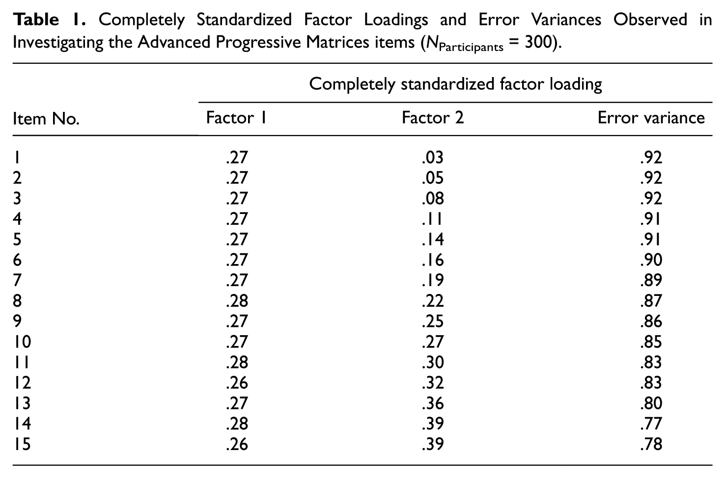
The loadings on the first factor were virtually constant and the ones on the second factor increased. The variance estimates of the two latent variables were 0.075 (t = 4.55, p < .05) and 0.166 (t = 3.99, p < .05) for basic ability and item-position effect. Since there was discrepancy between the asymptotic t statistics that were provided by LISREL and the observed variances, these variances were additionally scaled (Schweizer, 2011). In assuming average factor loadings of .3 for each factor the variance estimates were 0.128 (51%) and 0.122 (49%) for the first and second factors in corresponding order.

Discussion

The fit results observed in the investigation of the empirical data amounted to the conclusion that the second latent variable was indispensable for achieving a good account for the data. The CFI difference was so large that the presence of the second latent variable appeared to be beyond doubt. These results were in agreement with the outcomes of other studies aimed at identifying the item-position effect in scales composed of matrices items. However, although the used constraints favored the detection of the item-position factor, it could not be ruled out that the broad range of item difficulties was the source of variance leading to the additional factor.

Study 2: The Disentanglement of the Effects

This study served the disentanglement of the sources underlying the latent variables that represented the item-position effect and the wide range of items with various difficulties. The data matrices generated to be used in this investigation showed features of the data matrix of the first study: the number of columns corresponded to the number of items, the number of rows to the number of participants, and there was the same overall level of the covariances, that is, the mean of the numbers of the off-diagonal elements of the covariance matrix was the same. However, they differed from the empirical data matrix according to the range of item difficulties that was set to zero in the core study design. Therefore, the factor identified in addition to the basic ability factor could be assumed to reflect the item-position effect in following the logic of the modeling approach. To provide also evidence according to the experimental approach, there was variation of the pattern for data generation in addition to the breadth of the range of item difficulties, as is described by the extended study design.

Method

At first, three relational patterns were designed in considering major characteristics of the empirical data. The procedure described in the section on the estimation of the relational pattern served the achievement of one of these patterns. The similarity criterion c_broad-binary for checking the appropriateness (see Equation 3) was set to 0.005 since the overall level of the covariances appeared to be 0.05. The observed Euclidian distance of 0.003 satisfied this criterion. This high degree of similarity was achieved for v_C = 1.6875. The relational pattern achieved this way was referred to as the medium-level relational pattern (100%). Next two other relational patterns were derived by modifying the overall level in order to increase the generality of the results. The small-level relational pattern was achieved by a reduction of the sizes of the off-diagonal coefficients from 100% to 80% and the large-level relational pattern by an increase from 100% to 130%. The disproportional increase was selected because the medium level was rather close to zero but far away from one. In order to realize the extended study design, three uniform relational patterns were additionally generated. These patterns corresponded to the other patterns with the exception that the off-diagonal elements were uniform. Furthermore, pairs of uniform and nonuniform patterns corresponded according to the means of the off-diagonal elements.

The six relational patterns served the generation of the simulated data by means of the procedure described by Jöreskog and Sörbom (2001). The generation yielded three sets of 300 × 15 matrices of continuous and normally distributed random data (N(0, 1)). Since sets of 200 matrices could be considered to be sufficient for the cells of a design (Bandalos & Gagné, 2012), we generated 400 matrices with respect to each relational pattern. These matrices provided the starting point for dichotomization. The originally continuous data were replaced by ones or zeros depending on whether they were among the 50% larger numbers or 50% lower numbers. Since the replacement was the same for all columns of all matrices, the dichotomization could be expected to yield the zero range of item difficulties in all matrices of simulated data. To achieve a wide range of item difficulties, the columns of the matrices with continuous data were split according to the splits observed in the empirical example.

The investigation of the simulated data was conducted by means of the confirmatory factor models that already served the investigation of the matrices data of study 1. The same fit statistics and cutoffs were considered with the exception of TLI that turned out to be always very close to CFI. Again the comparison of the models including one and two latent variables was conducted by means of the CFI difference and the AICs.

Results

Results Regarding the Core Study Design

The results of investigating the simulated data showing the zero range of item difficulty by means of models representing the hypothesis that the data show the item-position effect are presented in Table 2.

Table 2.

Means and Standard Deviations (Within Parentheses) of the Fit Results for the Simulated Data Showing the Zero Range of Item Difficulty (N_Datasets = 400).

Level	N ^a	χ ²	df	Normed χ²	RMSEA	SRMR	CFI	GFI	N _diffCFI>0.01	N _AIC1>AIC2
Small	1	181.38 (23.59)	104	1.74 (0.23)	.049 (0.01)	.071 (0.01)	.77 (0.07)	.93 (0.01)
Small	2	163.46 (20.83)	103	1.58 (0.20)	.043 (0.01)	.066 (0.00)	.81 (0.07)	.94 (0.01)	378	395
Medium	1	233.16 (28.34)	104	2.24 (0.27)	.064 (0.01)	.079 (0.01)	.76 (0.06)	.91 (0.01)
Medium	2	204.30 (24.42)	103	1.98 (0.24)	.057 (0.01)	.073 (0.00)	.80 (0.05)	.93 (0.01)	396	400
Large	1	350.20 (37.17)	104	3.37 (0.36)	.089 (0.01)	.096 (0.01)	.73 (0.05)	.88 (0.01)
Large	2	298.30 (30.04)	103	2.90 (0.29)	.079 (0.01)	.085 (0.00)	.77 (0.05)	.90 (0.01)	398	400

Note. RMSEA = root mean square error of approximation; SRMR = standardized root mean square residual; CFI = comparative fit index; GFI = goodness-of-fit index; AIC, Akaike information criterion.

Number of latent variables.

The first to second rows give the results for the datasets constructed according to the relational pattern characterized by the small level of relations, the third to fourth rows for the datasets constructed in considering the medium level of relations and the fifth to sixth rows for the datasets with the large level. The first row of each set of two rows includes the means of the fit results for the 400 matrices obtained in confirmatory factor analysis according to the one-factor model; the corresponding standard deviations are given in parentheses. The second row of each set of rows comprises the fit results achieved by means of confirmatory factor analysis according to the two-factor model and the corresponding standard deviations are given in parentheses.

Virtually all mean normed chi-squares, RMSEAs, SRMRs, and GFIs indicated an acceptable or good model–data fit. In contrast, model misfit was signified by the CFI results. The outcomes of the comparison of the CFIs for the models with one and two latent variables are listed in the penultimate column as counts of the detections of the additional latent variable. The counts revealed that in 94.5%, 99%, and 99.5%, a substantial difference were observed for the matrices constructed according to the relational patterns showing the small, medium and large levels of relations, respectively. The results of comparing the AICs of the models with one and two latent variables are also presented as counts in the last column. These counts give the numbers of matrices showing a smaller AIC for the model with two latent variables than for the other model. According to these counts 98.75%, 100%, and 100% of the comparisons indicated the presence of the additional latent variable for matrices showing the small, medium, and large levels of relations, respectively.

Since the application of the modeling approach regarding the core study design within a simulation study gave rise to the expectation that the additional factor would be observed in virtually all investigations, the observed number of substantial results was compared with the maximum possible number by means of the χ² test for goodness of fit (Kanji, 1995). This test led to the χ² of 0.65 for the number comprising all CFI results while the critical value was 3.84 (p < .05). The application of this test to the AIC results yielded the χ² of 0.02 while the critical value was also 3.84 (p<.05). Both comparisons indicated that there was no substantial difference between the observed and expected counts.

Results Regarding the Extended Study Design

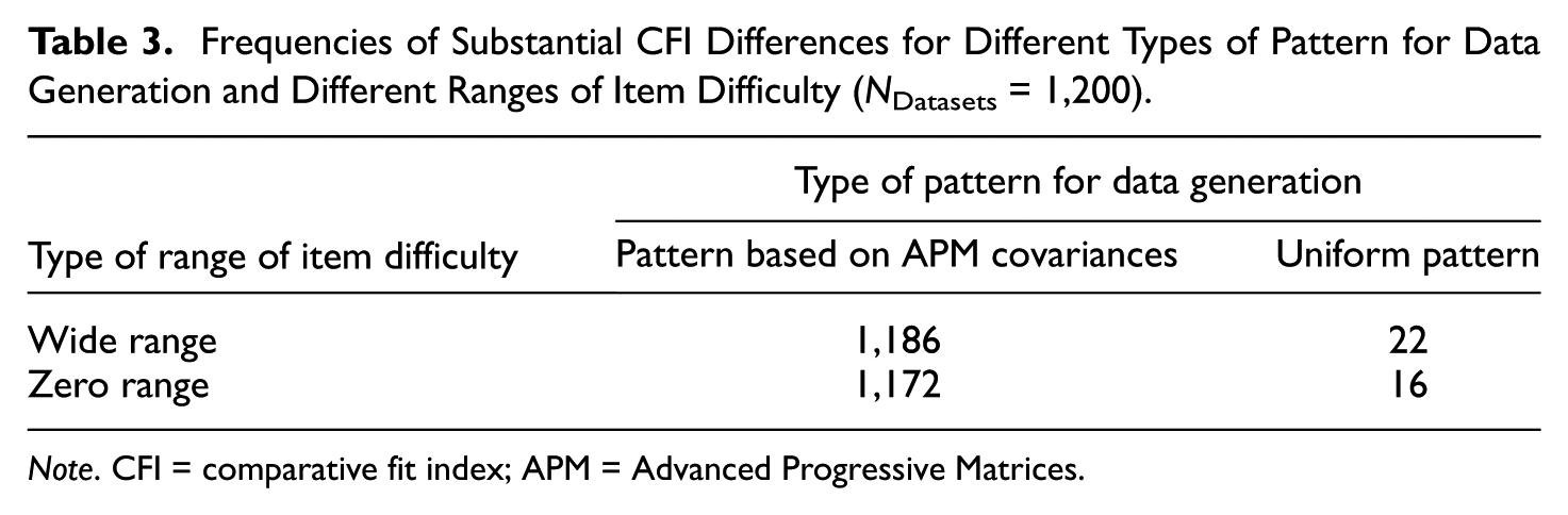
The CFI frequencies of detecting the additional latent variable in data showing variation according to the type of pattern used in data generation and the type of range of item difficulty are presented in Table 3.

Table 3.

Frequencies of Substantial CFI Differences for Different Types of Pattern for Data Generation and Different Ranges of Item Difficulty (N_Datasets = 1,200).

	Type of pattern for data generation
Type of range of item difficulty	Pattern based on APM covariances	Uniform pattern
Wide range	1,186	22
Zero range	1,172	16

Note. CFI = comparative fit index; APM = Advanced Progressive Matrices.

These frequencies originated from Table 3 and the corresponding tables of Appendices A -C. Furthermore, each frequency combined the counts for the three different relational levels.

The numbers reported in this table suggested a large effect according to the design factor associated with the item-position effect that was realized by different pattern for data generation. The χ² test for compatibility of k counts (Kanji, 1995) yielded for this design factor the χ² of 2246.4 while the critical value was 3.84 (p < .05). Regarding the second design factor associated with the effect originating from the item difficulties and realized as the types of range of item difficulty, the χ² was 0.17. The comparison of this value with the critical value that was also 3.84 (p < .05) led to the conclusion that the effect of the range of item difficulties was negligible.

Finally, the investigation of AIC frequencies led to similar but a bit less clear results because the lack of a confidence interval (see Appendix D).

Discussion

In almost all matrices of simulated data constructed in accordance with the empirical example of the first study, the presence of the additional factor was indicated although the broad range of item difficulties is missing. The presence of this factor was obvious from the outcomes of the CFI and AIC comparisons according to the core study design with minor discrepancies only. This outcome was confirmed by the results of the investigation according to the extended study design. The comparison regarding the item-position design factor revealed a large difference between the level representing the assumption of the item-position effect and the level of no such assumption. Furthermore, no difference was indicated for the difficulty design factor. Although the frequencies showed some more observations of the additional latent variable when the range of item difficulties was wide, the difference was far from reaching the level of significance.

The results of this study were in line with the results of the IRT studies that were conducted to find out about a possible mix-up of the effects due to the item-position effect and the effect due to the item difficulties (for an overview, see Kubinger, 2009). In contrast, in the research by means of factor analysis so far the item-position factor and the difficulty factor were investigated independently of each other so that it is not possible to check the agreement with previous results.

General Discussion

The possible mix-up of the difficulty factor and the factor due to the item-position effect calls the validity of the assumption that the additional factor observed in investigating the structure is the due to the item-position effect into question. Because of the similar preconditions of these factors to arise, the assertion that the difficulty factor is an alternative explanation for the observed additional factor cannot simply be rejected. Although the idea of the difficulty factor has virtually disappeared from the scientific discussion in recent years, as is obvious from the low number of hits in literature research for the last decade, it must be taken seriously. The neglect is probably due to the increased sensitivity for the appropriateness of the scale in data analysis and the consequences for statistical investigations (Skrondal & Rabe-Hesketh, 2004). It even appears that this kind of sensitivity has meanwhile resulted into a reduced use of CFA for investigating such data.

The wide range of items with various difficulties is one alternative explanation for the additional factor that should not be confused with the explanation highlighting the ordering of the items according to their difficulties additionally. In the first case the ordering does not count whereas in the second case the ordering is important together with the wide range of items with various difficulties. This further explanation has stimulated a number of IRT studies by means of the linear logistic test model (e.g., Hohensinn et al., 2008; Hohensinn, Kubinger, Reif, Schleich, & Khorramdel, 2011). Data obtained by means of different ability scales were investigated to find out about the validity of this explanation. The outcomes of most studies do not support this explanation (for an overview see Kubinger, 2009). However, the reported IRT based findings may only be of limited values in the factor-analytic framework because of the different foci: IRT investigations focus on the probabilities of items and CFA investigations on the systematic variances. Additionally, the difficulty factor problem seems to be unique for factor analysis. Furthermore, the results of Knowles’s (1988) seminal study suggest that there is no such ordering effect. It is a characteristic of Knowles’s study that the data stem from the application of different versions of an item lists achieved by changing the ordering systematically for data collection.

Regarding the present investigation, it can be stated that the shift away from the wide range to the zero range of item difficulties that means the manipulation of the design factor reflecting the configurations of the item difficulties did not lead to the disappearance of the additional factor. The apparent stability of the additional factor suggests that it represents the item-position effect. Although the average chi-square difference of the models with one and two latent variables was somewhat larger in the original data (32.4) than in the simulated data (28.9), the mean difference between the model assuming one latent variable and the model assuming two latent variables is still remarkable. According to this observation, the source of the item-position effect appears to be much stronger than the wide range of items with various difficulties. However, a cautionary note needs to be added. In this study, the small size of the effect of the wide range of items of various difficulties leading to the difficulty factor may partly be due to the constraint of the factor loadings. The constraints of the item-position factor only allow subsets of items of the same difficulty to contribute additionally to the difficulty factor if they are located in the area of the scale where the item-position effect is expected to be especially strong. In investigations using other models of measurement much stronger effects may be observed due to the wide range of items with various difficulties in combination with subsets showing the same difficulty. Hence according to the results of the present study there is reason for concluding that an additional factor in a homogeneous performance test is much more likely to be the item-position factor than the difficulty factor.

Finally, we like to indicate that the range of applications of the described methods is not restricted to cases of insecurity regarding the source of the additional factor if the alternatives are the difficulty factor and the item-position factor. The application of this method can also be useful if a structural investigation does not reveal the expected homogeneity. In larger numbers of items there is always some change that an additional factor may arise (Davis-Stober, Doignon, & Suck, 2015) since there may be inhomogeneity due to subsets of very similar items. Such inhomogeneity is likely to lead to model misfit.

Footnotes

Appendix

Appendix D

Frequencies of AIC differences Favoring the Two-Factor Model for Different Types of Pattern for Data Generation and Different Ranges of Item Difficulty (N_Datasets = 1,200).

	Type of pattern for data generation
Type of range of item difficulty	Pattern based on APM covariances	Uniform pattern
Wide range	1,198	266
Zero range	1,195	181

Note. AIC = Akaike information criterion; APM = Advanced Progressive Matrices.

Declaration of Conflicting Interests

The author(s) declared no potential conflicts of interest with respect to the research, authorship, and/or publication of this article.

Funding

The author(s) disclosed receipt of the following financial support for the research, authorship, and/or publication of this article: The first author was supported by Deutsche Forschungsgemeinschaft, Grant SCHW 402/20-1.

References

Bandalos

D. L.

Gagné

(2012). Simulation methods in structural equation modeling. In Rick

R. H.

(Ed.), Handbook of structural equation modeling (pp. 92-108). New York, NY: Guilford Press.

Bandalos

D. L.

Gerstner

J. J.

(2016). Using factor analysis in test construction. In Schweizer

DiStefano

(Eds.), Principles and methods of test construction (pp. 26-51). Göttingen, Germany: Hogrefe.

Campbell

D. T.

Mohr

P. J.

(1950). The effect of ordinal position upon responses to items in a check list. Journal of Applied Psychology, 34, 62-67. doi:10.1037/h0061818

Carlstedt

Gustafsson

J.-E.

Ullstadius

(2000). Item sequencing effects on the measurement of fluid intelligence. Intelligence, 28, 145-160. doi:10.1016/S0160-2896 (00)00034-9

Chen

F. F.

(2007). Sensitivity of goodness of fit indexes to lack of measurement invariance. Structural Equation Modeling, 14, 464-504. doi:10.1080/10705510701301834

Cheung

G. W.

Rensvold

R. B.

(2002). Evaluating goodness-of-fit indexes for testing measurement invariance. Structural Equation Modeling, 9, 233-255. doi:10.1207/S1532 8007SEM0902_5

Davis-Stober

C. P.

Doignon

J.-P.

Suck

(2015). A note on the eigensystem of the covariance matrix of dichotomous Guttman items. Frontiers in Psychology. doi:10.3389/fpsyg.2015.01767

Debeer

Janssen

(2013). Modeling item-position effects within an IRT framework. Journal of Educational Measurement, 50, 164-185. doi:10.1111/jedm.12009

DiStefano

(2016). Examining fit with structural equation models. In Schweizer

DiStefano

(Eds.), Principles and methods of test construction (pp. 26-51). Göttingen, Germany: Hogrefe.

10.

DiStefano

Motl

R. W.

(2006). Further investigating method effects associated with negatively worded items on self-report surveys. Structural Equation Modeling, 13, 440-464. doi:10.1207/s15328007sem1303_6

11.

Embretson

S. E.

(1991). A multidimensional latent trait model for measuring learning and change. Psychometrika, 56, 495-515. doi:10.1007/BF02294487

12.

Ferguson

G. A.

(1941). The factorial interpretation of test difficulty. Psychometrika, 6, 323-329. doi:10.1007/BF02288588

13.

Floyd

F. J.

Widaman

K. F.

(1995). Factor analysis in the development and refinement of clinical assessment instruments. Psychological Assessment, 7, 286-299. doi:10.1037/1040-3590.7.3.286

14.

Gibson

W. A.

(1960). Nonlinear factors in two dimensions. Psychometrika, 25, 381-392. doi:10.1007/BF02289755

15.

Gittler

Wild

(1989). Der Einsatz des LLTM bei der Konstruktion des Itempools für das adaptive Testen [The use of LLTM for the construction of an item pool for adaptive testing]. In Kubinger

K. D.

(Ed.), Moderne Testtheorie—Ein Abriss samt neuesten Beiträgen (pp. 115-139). Munich, Germany: PVU.

16.

Hartig

Hölzel

Moosbrugger

(2007). A confirmatory analysis of item reliability trends (CAIRT): differentiating true score and error variance in the analysis of item context effects. Multivariate Behavioral Research, 42, 157-183. doi:10.1080/00273170701341266

17.

Hohensinn

Kubinger

K. D.

Reif

Holocher-Ertl

Khorramdel

Frebort

(2008). Examining item-position effects in large-scale assessment using the linear logistic test model. Psychology Science Quarterly, 50, 391-402.

18.

Hohensinn

Kubinger

K. D.

Reif

Schleich

Khorramdel

(2011). Analysing item position effects due to test booklet design within large-scale assessment. Educational Research and Evaluation, 17, 497-509. doi:10.1080/13803611.2011.632668

19.

Bentler

P. M.

(1999). Cutoff criteria for fit indexes in covariance structure analysis: conventional criteria versus new alternatives. Structural Equation Modeling, 6, 1-55. doi:10.1080/10705519909540118

20.

Jöreskog

K. G.

(1970). A general method for analysis of covariance structure. Biometrika, 57, 239-257. doi:10.2307/2334833

21.

Jöreskog

K. G.

(1971). Statistical analysis of sets of congeneric tests. Psychometrika, 36, 109-133. doi:10.1007/BF02291393

22.

Jöreskog

K. G.

Sörbom

(2001). Interactive LISREL: User’s guide. Lincolnwood, IL: Scientific Software International.

23.

Jöreskog

K. G.

Sörbom

(2006). LISREL 8.80. Lincolnwood, IL: Scientific Software International.

24.

Kanji

G. K.

(1995). Statistical tests. London, England: Sage.

25.

Kenny

D. A.

Kashy

D. A.

(1992). Analysis of the multitrait-multimethod matrix by confirmatory factor analysis. Psychological Bulletin, 112, 165-172. doi:10.1037/0033-2909.112.1.165

26.

Kishton

J. M.

Widaman

K. F.

(1994). Unidimensional versus domain representative parceling of questionnaire items: An empirical example. Educational and Psychological Measurement, 54, 757-765. doi:10.1177/0013164494054003022

27.

Kline

R. B.

(2005). Principles and practice of structural equation modeling (2nd ed.). New York, NY: Guilford Press.

28.

Knowles

E. S.

(1988). Item context effects on personality scales: Measuring changes the measure. Journal of Personality and Social Psychology, 55, 312-320. doi:10.1037/0022-3514.55.2.312

29.

Knowles

E. S.

Byers

(1996). Reliability shifts in measurement reactivity: Driven by content engagement or self-engagement?Journal of Personality and Social Psychology, 70, 1080-1090. doi:10.1037/0022-3514.70.5.1080

30.

Kubinger

K. D.

(2009). Applications of the linear logistic test model in psychometric research. Educational and Psychological Measurement, 69, 232-244. doi:10.1177/0013164408322021

31.

Kubinger

K. D.

Formann

A. K.

Farkas

M. G.

(1991). Psychometric shortcomings of Raven’s Standard Progressive Matrices SPM) in particular for computerized testing. European Review of Applied Psychology, 41, 295-300.

32.

Lord

F. M.

Novick

M. R.

(1968). Statistical theories of mental test scores. Reading, MA: Addison-Wesley.

33.

Lozano

J. H.

(2015). Are impulsivity and intelligence truly related constructs? Evidence based on the fixed-links model. Personality and Individual Differences, 85, 192-198. doi:10.1016/j.paid.2015.04.049

34.

Lucke

J. F.

(2005). The α and ω of congeneric test theory: An extension of reliability and internal consistency to heterogeneous tests. Applied Psychological Measurement, 29, 65-81. doi:10.1177/0146621604270882

35.

Marsh

H. W.

(1989). Confirmatory factor analysis of multitrait-multimethod data: Many problems and a few solutions. Applied Psychological Measurement, 13, 335-361. doi:10.1177/014662168901300402

36.

Marsh

H. W.

Bailey

(1991). Confirmatory factor analyses of multitrait-multimethod data: A comparison of alternative models. Applied Psychological Measurement, 15, 47-70. doi:10.1177/014662169101500106

37.

McDonald

R. P.

(1965). Difficulty factors and nonlinear factor analysis. British Journal of Mathematical and Statistical Psychology, 18, 11-23. doi:10.1111/j.2044-8317.1965 .tb00690.x

38.

McDonald

R. P.

Ahlawat

K. S.

(1974). Difficulty factors in binary data. British Journal of Mathematical and Statistical Psychology, 27, 82-99. doi:10.1111/j.2044-8317.1974 .tb00530.x

39.

Mollenkopf

W. G.

(1950). An experimental study of the effects on item analysis data of changing item placement and test-time limit. Psychometrika, 15, 291-315. doi:1007/BF02289044

40.

Rasch

(1960). Probabilistic models for some intelligence and attainment tests. Copenhagen, Denmark: Danish Institute for Educational Research.

41.

Raven

J. C.

Raven

Court

J. H.

(1997). Raven’s progressive matrices and vocabulary scales. Edinburgh, Scotland: J. C. Raven.

42.

Ren

Goldhammer

Moosbrugger

Schweizer

(2012). How relates attention to the ability-specific and position-specific components of reasoning measured by APM?Learning and Individual Differences, 22, 1-7. doi: 10.1016/j.lindif.2011.09.009

43.

Schweizer

(2011). Scaling variances of latent variables by standardizing loadings: Applications to working memory and the position effect. Multivariate Behavioral Research, 46, 938-955. doi:10.1080/00273171.2011.625312

44.

Schweizer

(2012). The position effect in reasoning items considered from the CFA perspective. International Journal of Educational and Psychological Assessment, 11, 44-58.

45.

Schweizer

(2013). A threshold-free approach to the study of the structure of binary data. International Journal of Statistics and Probability, 2, 67-75. doi:10.5539/ijsp.v2n2p67

46.

Schweizer

Ren

Wang

(2015). A comparison of confirmatory factor analysis of binary data on the basis of tetrachoric correlations and of probability-based covariances: A simulation study. In Millsap

R. E.

Bolt

D. M.

van der Ark

L. A.

Wang

W.-C.

(Eds.), Quantitative psychology research (pp. 273-292). Heidelberg, Germany: Springer.

47.

Schweizer

Ren

Wang

Zeller

(2015). Does the constraint of factor loadings impair model fit and accuracy in parameter estimation?International Journal of Statistics and Probability, 4, 40-50. doi:10.5539/ijsp.v4n4p40

48.

Schweizer

Schreiner

Gold

(2009). The confirmatory investigation of APM items with loadings as a function of the position and easiness of items: a two-dimensional model of APM. Psychology Science Quarterly, 51, 47-64.

49.

Skrondal

Rabe-Hesketh

(2004). Generalized latent variable modelling: Multilevel, longitudinal and structural equation models. Boca Raton, FL: Chapman & Hall/CRC Press.

50.

Vautier

Steyer

Jmel

Raufaste

(2005). Imperfect or perfect dynamic bipolarity? The case of antonymous affective judgements. Structural Equation Modeling, 12, 391-410. doi:10.1207/s15328007sem1203_3

51.

Verguts

De Boeck

(2000). A Rasch model for detecting learning while solving an intelligence test. Applied Psychological Measurement, 24, 151-162. doi:10.1177/014662 10022031589

52.

Vogt

W. P.

(2005). Dictionary of statistics & methodology: A nontechnical guide for the social sciences (3rd ed.). Thousand Oaks, CA: Sage.

53.

Widaman

K. F.

(1985). Hierarchically nested covariance structure models for multitrait-multimethod data. Applied Psychological Measurement, 10, 1-22. doi:10.1177/014662 168500900101