
Abstract
Stan is a new Bayesian statistical software program that implements the powerful and efficient Hamiltonian Monte Carlo (HMC) algorithm. To date there is not a source that systematically provides Stan code for various item response theory (IRT) models. This article provides Stan code for three representative IRT models, including the three-parameter logistic IRT model, the graded response model, and the nominal response model. We demonstrate how IRT model comparison can be conducted with Stan and how the provided Stan code for simple IRT models can be easily extended to their multidimensional and multilevel cases.
Introduction
In the past two decades, Bayesian item response theory (IRT) modeling has become increasingly popular due to the advance of computing power and the Markov chain Monte Carlo (MCMC) algorithms. Multiple software programs became available to implement some MCMC algorithms, including WinBUGS (Lunn, Thomas, Best, & Spiegelhalter, 2000), OpenBUGS (Spiegelhalter, Thomas, Best, & Lunn, 2010), JAGS (Plummer, 2003), PROC MCMC in SAS, and Mcmcpack (Martin, Quinn, & Park, 2011) in R. In those software programs, the Gibbs sampling (Geman & Geman, 1984) and the Metropolis algorithm (Metropolis, Rosenbluth, Rosenbluth, Teller, & Teller, 1953) are most frequently used. Despite their popularity, these sampling algorithms have some limitations as well, especially the long computation time required for model convergence due to their inefficiency in exploring the posterior parameter space (Neal, 1993).
Stan (Carpenter et al., 2017) is a new Bayesian software program implementing the no-U-turn sampler (Hoffman & Gelman, 2014), an extension to the Hamiltonian Monte Carlo (HMC; Neal, 2011) algorithm. HMC is considerably faster than the Gibbs sampler and the Metropolis algorithm because it explores the posterior parameter space more efficiently. It does so by pairing each model parameter with a momentum variable, which determines HMC’s exploration behavior of the target distribution based on the posterior density of the current drawn parameter value 1 and hence enables HMC to “suppress the random walk behavior in the Metropolis algorithm” (Gelman, Carlin, Stern, & Rubin, 2014, p. 300). Consequently, Stan is considerably more efficient than the traditional Bayesian software programs. As stated in the Stan User Manual (Stan Development Team, 2016a, p. 541), “Stan might work fine with 1000 iterations with an example where BUGS would require 100,000 for good mixing.” Another advantage of Stan is that unlike WinBUGS and OpenBUGS, it does allow the use of improper priors. In addition, it allows interface with other software programs such as R, Python, Matlab, Stata, Julia, as well as its compatibility with all three major operating platforms, namely Linux, Mac, and Windows.
Curtis (2010) introduced WinBUGS codes for several IRT models while other researchers (Ames & Samonte, 2015; Stone & Zhu, 2015) presented on using SAS PROC MCMC for IRT model parameter estimation. Despite its efficiency and easy accessibility in different interfaces, no article collectively introduces Stan codes for IRT model parameter estimation. Stan user manual (Stan Development Team, 2016a) introduces the one-parameter logistic (1PL) and two-parameter logistic (2PL) IRT models. However, if one is interested in extended IRT models, it may take a long time to learn the basics and figure out these extensions.
To promote the accessibility of Stan, this article intends to present Stan codes for three more generalized IRT models and their multidimensional and multilevel extensions. The three models are the three-parameter logistic (3PL) dichotomous IRT model, the graded response model (GRM), and the nominal response model (NRM).
2
Essentially, the 3PL model is a general case for dichotomous item responses while the other two polytomous IRT models are the difference models and the divide-by-total models, respectively (Thissen & Steinberg, 1986). Other dichotomous IRT models such as the 1PL and 2PL IRT models, and polytomous IRT models such as the partial credit model (Masters, 1982) and the rating scale model (Andrich, 1978) can be easily developed by modifying the Stan codes provided. With the introduction to the multilevel and multilevel extensions, many more available IRT models could be possible. Furthermore, this article specifically focuses on
The rest of this article is organized into three parts. The first part describes the basic components of a Stan program and the codes for the three IRT models. The second part illustrates with both real and simulated data sets how to conduct model comparison and fit multidimensional and multilevel IRT models in Stan. This article concludes with a discussion regarding the use and limitations of Stan.
Components of a Stan Program
The main function in the
Data Block
The first necessary component of a Stan model is the data block, in which a researcher specifies the relevant data information and the data itself. The data block, as well as any other block in a Stan file, contains a pair of curly brackets “{ }” in which Stan codes are written. For dichotomous IRT models, three pieces of information are usually provided in the data block: the number of examinees, the number of items, and a response matrix (Listing 1, lines 2-4) as follows:

For polytomous IRT models, the number of categories for each item, which is an integer if all items have the same number of categories or a vector of integers for items with different response categories (Listing 2-3, lines 2-5), needs to be specified. One big difference between Stan and BUGS is that data type has to be specified in Stan. The number of students and the number of items are specified as int (integers), while the response matrix is specified to be an array of integers, followed by its dimension. As the polytomous items in the demo codes contain four response categories, the number of categories is specified as an integer (e.g., Listing 2, line 2).
Stan provides an extra layer of data check by allowing the user to provide a data boundary in a pair of angle brackets “< >” after the specification of data type. For example, in the 3PL model, the elements in the response matrix are specified to range from 0 to 1 (Listing 1, line 4). If one element in the matrix has a value of 2, Stan will produce a warning message to notify the user that some value in the response matrix is out of range. Similarly, in a polytomous IRT model, the elements in the response matrix ranging from one to the number of categories should be specified accordingly in the data block (e.g., Listing 2, line 5).
Parameters Block
Following the data block is the parameters block in which model parameters are specified. In the context of IRT, model parameters usually include latent ability and item parameters such as difficulty, discrimination, and pseudoguessing parameters. Hyperparameters in the priors for any model parameters need to be specified in this block as well. If any model parameter or hyperparameter that appears in the subsequent model block is not specified in this block, Stan will provide warnings that a particular variable is not found and stop. Therefore, it is essential that a Stan user knows what model parameters and hyperparameters (if any) are in the model of interest and specify them accordingly and exhaustively. In the following, we provide a brief description of each of the three IRT models, followed by a discussion of how the corresponding model parameters and hyperparameters are specified.
The 3PL IRT model can be expressed as
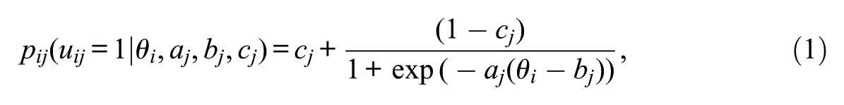
where
Model parameters in the 3PL IRT model that need to be specified in the parameter block include all the parameters on the right side of Equation (1) (Listing 1, lines 7-10) and their hyperparameters. In this illustration, a normal distribution with unknown mean (mu_beta) and unknown standard deviation (sigma_beta) is specified as a prior for the item difficulty parameter and a lognormal distribution with a mean of zero and unknown standard deviation (sigma_alpha) for the discrimination parameter. Consequently, the parameters block includes three lines for these three hyperparameters (Listing 1, lines 11-13) as follows:

The graded response model (GRM; Samejima, 1969) can be viewed as a generalized case of the 2PL IRT model in that it allows more than two response categories in an item. Instead of directly modeling the probability of a response of a certain response category, GRM first models the probability of responding below a certain category versus above that category. The difference of such probabilities is the probability of responding at that category. The mathematical equation for GRM is given as
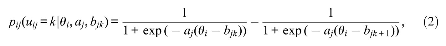
where k refers to the kth category,
Similarly, all the GRM model parameters on the right side of Equation (2) are specified in this block (Listing 2, lines 8-10). The prior distribution for item difficulty contains two hyperparameters, and they are specified in this block as well (Listing 2, lines 11-12). The category difficulty parameter
The nominal response model (NRM; Bock, 1972) takes the form

where
The data type for all parameters in the parameters block need to be specified. If one of the model parameters is defined as a vector or a matrix, its dimension needs to be specified. For example, in the 3PL IRT model, the ability parameter (theta) is specified to be a vector with a length equal to the number of students (Listing 1, line 7). In addition, if a parameter is expected to be within a certain range, the range should be provided right after the data type. For example, the pseudoguessing parameter of the 3PL model (gamma) is constrained to range from 0 to 1 (Listing 1, line 10). In the GRM, the standard deviation of the prior for the category difficulty parameter (sigma_kappa) is constrained to be nonnegative (Listing 2, line 12).
Model Block
The model block, where the priors and the model are specified, is the most essential component of a Stan program. Note that all the parameters appearing in this block have to be specified in advance in the parameters block, or Stan will produce an error message and stop. Prior distributions for all the parameters in the parameter block need to be specified. If a prior is not specified, a uniform prior will be automatically assumed by Stan. For example, we use a standard normal distribution as a prior for the ability parameters (theta) in the 3PL model (Listing 1, line 16), and a normal distribution with unknown mean (mu_beta) and unknown standard deviation (sigma_beta) for the item difficulty parameters (beta; Listing 1, line 17). The hyperprior for mu_beta is specified as a normal distribution with a mean of 0 and standard deviation of 5 (Listing 1, line 18), and a Cauchy distribution as a hyperprior for sigma_beta (Listing 1, line 19). Note that since sigma_beta has been constrained to be nonnegative in the parameters block (Listing 1, line 13), this Cauchy distribution as a hyperprior is actually a half Cauchy distribution. Similar to any other Bayesian software program, the priors may be informative, weakly informative, or noninformative, and the choice should reflect our belief about those parameters.
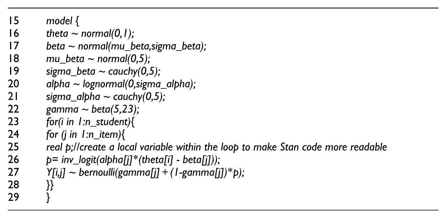
After all priors and hyperpriors have been specified, the model is specified in the sampling statement through a function. Three functions, including bernoulli (Listing 1, line 27), ordered_logistic (Listing 2, line 25), and categorical_logit (Listing 3, line 29), are used for the 3PL model, the GRM, and the NRM, respectively. Since the bernoulli function is the Stan analog of the dbern function in BUGS, we focus our discussion on ordered_logistic and categorical_logit here.
The function categorical_logit is a direct parameterization of categorical, which is the Stan counterpart of the function dcat in BUGS. Such a parameterization is “numerically more stable if the chance of success parameter is on the logit scale . . .” (Stan Development Team, 2016a, p. 409). The function categorical_logit can be used for all polytomous IRT models that belong to the divide-by-total family. For the NRM, categorical_logit(zetan[j]+lambdan[j]*theta[i]) (Listing 3, line 29) is equivalent to categorical(
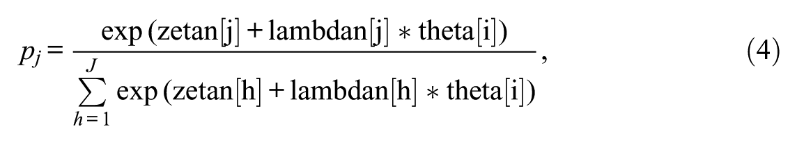
where the terms other than notational differences, are the same as those in Equation (3).
The function ordered_logistic in the GRM (Listing 2, line 25), combined with the category difficulty parameter kappa specified as the ordered data type in the parameters block (Listing 2, line 10), leads to a mathematical equation that is identical to Equation (2), with the category difficulty parameter
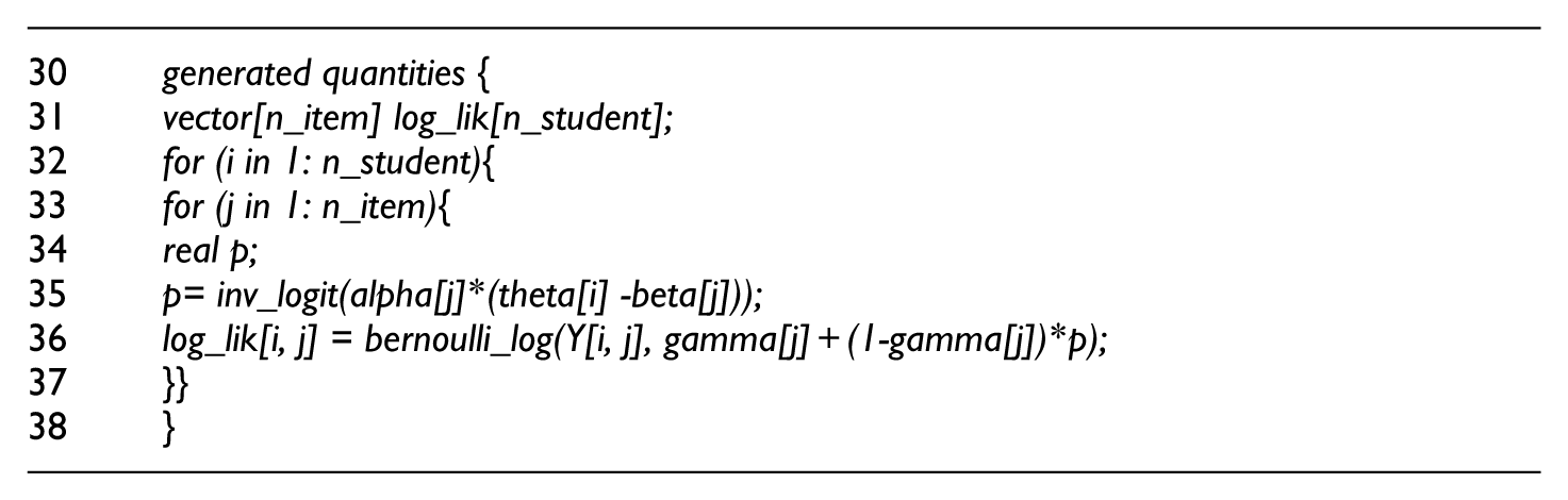
Generated Quantities Block
The generated quantities block is an optional component of the Stan code, and it is usually used when there is a need to compute new variables and obtain their corresponding posterior distributions. In the IRT context, this block can be used to compute the model-based log-likelihood, which is used for the computation of model fit indices for model comparison and selection purposes. The computation of model-based log-likelihood requires the use of a function that is the combination of the function used in the sampling statement and a suffix “log.” For example, in the generated block section of the 3PL model (Listing 1, lines 30-38), the function bernoulli_log (Listing 1, line 36) is used, which is the function bernoulli used in the sampling statement of the model block (Listing 1, line 27) plus the suffix “log.” The generated quantity block included for all the three IRT models in this article can be deleted if model comparison and selection is not of interest.
With the log-likelihood specified in this block, their posterior distributions can be obtained and used to compute the widely available information criterion (WAIC; Watanabe, 2010) and leave-one-out cross-validation (LOO; Vehtari, Gelman, & Gabry, 2016a). In BUGS, model comparison is usually conducted using the deviance information criterion (DIC; Spiegelhalter, Best, Carlin, & van der Linde, 2002). Stan does not compute DIC for model comparison and selection purposes; instead, it uses WAIC and LOO, which are fully Bayesian and theoretically superior to traditional information-based model selection criteria such as the Akaike information criterion (AIC; Akaike, 1974), the Bayesian information criterion (BIC; Schwarz, 1978), and DIC. In the context of IRT model selection, Luo and Al-Harbi (2016) investigated the performances of WAIC and LOO in choosing the correct dichotomous IRT models and found that they were superior to the more traditional methods such as the likelihood ratio test, AIC, BIC, and DIC. The computation of WAIC and LOO can be intensive and nontrivial, and approximation methods usually have to be used. Fortunately, an R package
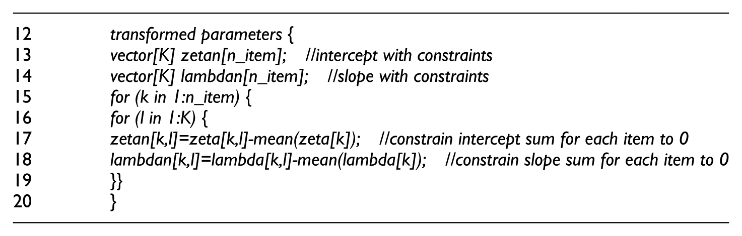
Transformed Parameters Block
The transformed parameters block is optional too and used when some parameters specified in the parameters block need to be transformed. A transformed parameter in this block is usually constrained to be a function of some other parameters in the parameters block, and imposing a prior distribution on such a constrained parameter in the subsequent model block causes Stan to produce an error message and stop, which is another notable difference between Bugs and Stan. Consequently, it is necessary in Stan to separate the freely estimated parameters and the constrained parameters into the parameters block and the transformed parameters block, respectively.
In the IRT context, this block is often used for model identification purposes. For example, models that are members of the Rasch family can use this block to constrain the sum of item difficulty parameters to be 0. Among the three IRT models illustrated in this article, the NRM is the only one that requires the transformed parameter block to identify the model by constraining both the sum of category intercepts and that of category slopes for each item to be 0. One way to set the sum of all intercept parameters for an item to be 0 is to constrain the last intercept parameter to be the negative sum of the remaining intercept parameters of that particular item. In the example code, a different approach (e.g., Bolt, Cohen, & Wollack, 2001) is followed by creating new sets of intercept and slope parameters which are deviations from the means of the original intercept and slope parameter specified in the parameters block (Listing 3, lines 17-18) as the following presented lines. Note that while the transformed parameters (lambdan and zetan) are directly used in the sampling statement to describe the model of interest (Listing 3, line 29), only the parameters in the parameters block from which they are transformed (lambda and zeta) are given priors (Listing 3, lines 23-26).
Illustrations for Unidimensional Dichotomous, Multidimensional Testlet and Multilevel IRT Models
In this section, both real and simulated data sets are used to demonstrate how to use Stan to analyze dichotomous item response data using unidimensional IRT model, multidimensional testlet model, and multilevel IRT model. We assume that the
Example 1: Model Comparison
The data set used in this example is from a high-stakes English proficiency test in a Middle-Eastern country for admission and placement purposes, consisting of four sections including listening, reading comprehension, sentence completion, and grammar. All items are multiple-choice questions. For illustration of model comparison, we only used response data from the listening section which contains 20 items with a sample size of 1,637.
The code for conducting model comparison is provided in Listing 4. First the working directory in R is set up and the
Assuming the data set has been already saved as a comma-separated values (csv) file in the directory folder, the data are imported and its dimension (which indicates the number of students and items in the data set) is extracted (Listing 4, lines 6-8). A data list is created to include the number of students, the number of items, and the response matrix (Listing 4, line 9). It should be noted that the name assigned in the data list must match what is provided in the data block of a Stan program. Otherwise Stan will produce an error message. For example, here the response matrix is named as Y, and in the Stan code for the 3PL IRT model the same Y is found (Listing 1, line 4).
Four arguments for the function stan in
Running
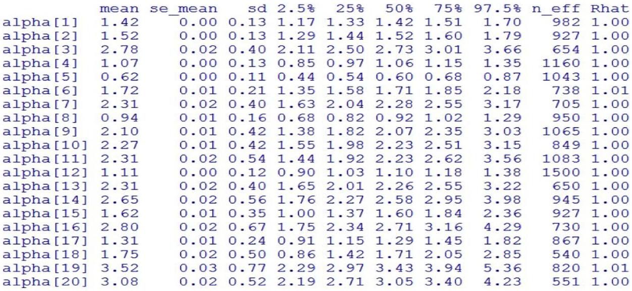
Estimates of item discrimination parameters in the three-parameter logistic item response theory (3Pl IRT) model.
The trace plots for model parameters can be requested with the function traceplot in
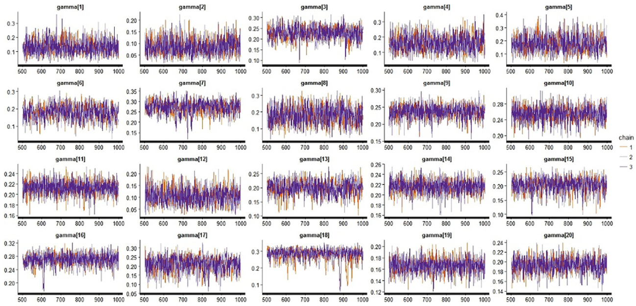
Trace plots of the pseudoguessing parameters in the three-parameter logistic item response theory (3PL IRT) model.
In general,
After confirming model convergence, WAIC and LOO are computed in lines 15 to 23 in Listing 4 for each compared model. As the log-likelihood has been computed in the generated quantity block, the function extract_log_lik can be used to directly extract the posterior distribution of the log-likelihood (Listing 4, lines 15, 18, and 21) and then WAIC and LOO are computed with the functions waic and loo, respectively (e.g., Listing 4, lines 16-17). Table 1 lists the WAIC and LOO values for the three dichotomous IRT models, both of which lead to the same conclusion that the 3PL IRT model has the smallest values of LOO and WAIC. Consequently, it was concluded that the 3PL IRT model was the best-fitting model among the three competing dichotomous IRT models.
WAIC and LOO for Three Dichotomous Item Response Theory Models.
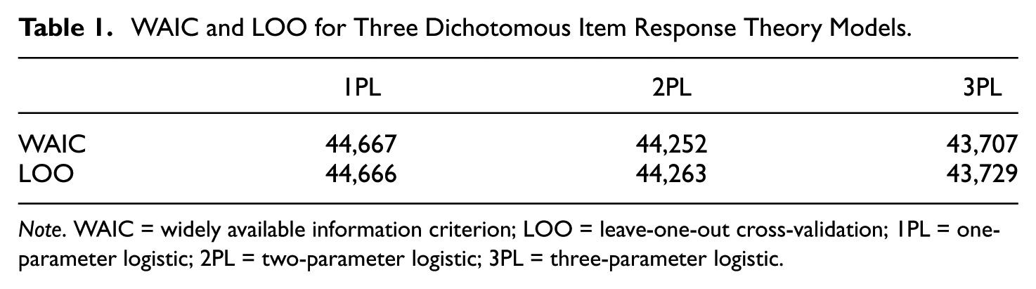
Note. WAIC = widely available information criterion; LOO = leave-one-out cross-validation; 1PL = one-parameter logistic; 2PL = two-parameter logistic; 3PL = three-parameter logistic.
Example 2: The Rasch Testlet Model
This example demonstrates how to use
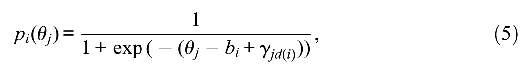
where
Listing 5 provides the R code for the analysis in this example. The data are transposed and the number of items and the number of examinees are extracted in lines 6 to 8 in Listing 5. Such data transposing makes Stan more efficient as illustrated below. The number of testlets or item groups is specified in a data list named data_testlet in lines 9 to 11 of Listing 5.
Stan code for the Rasch testlet model can be saved as an external file and runs in the stan function. Another way is to specify the Stan program for the Rasch testlet model as an object called code_testlet in the R environment as in lines 12 to 45 of Listing 5. This Stan program is similar to that for the 3PL IRT model except the inclusion of the number of testlets and the item group membership as specified in lines 15 to 16 of Listing 5 in the data block. In the parameter block, two parameters, gamma and sd_gamma are specified for the testlet parameters and the testlet variance, respectively (Listing 5, lines 21 and 24). In the model block, normal distributions are assumed as priors for
This example uses the transformed parameters block to constrain the sum of item difficulty parameters to be zero (Listing 5, line 30) for model identification. In addition, the function bernoulli_logit is used (Listing 5, line 42) in the sampling statement. This function is a direct parameterization of bernoulli and can be used for both 1PL and 2PL IRT models. For the 2PL IRT model, it is expressed as bernoulli_logit(alpha[j]*(theta[i]- beta[j])), which is equivalent to bernoulli(1/(1+exp(-alpha[j]*(theta[i]- beta[j])))). For the 3PL IRT model, the function bernoulli_logit cannot be used due to the addition of the lower-asymptote parameter.
Different from that specified for the above three IRT models, the sampling statement for the Rasch testlet model (Listing 5, lines 41-43) is vectorized for efficiency. In the sampling statement for the first three models (e.g., Listing 1, lines 22-25), a double loop is used to model one element at a time from the response matrix. This example demonstrates that a single loop is used to model one vector (its length is the number of examinees) at a time from the response matrix. Such a vectorized sampling statement improves computation efficiency in Stan because “. . . vectorized log probability functions are faster than their equivalent form defined with loops” (Stan Development Team, 2016a, p. 405).
The sampling statement in this example (Listing 5, line 42) warrants some additional explanation. With the data transposed (Listing 5, line 6), res[i] outputs the vector of all examinees’ responses to item i with a length equal to the number of examinees. The parameter theta is defined as a vector with the same length (Listing 5, line 20), and gamma[t_index[i]] indicates a specific testlet that item i is associated with and the vector of the testlet effect with the same length as the number of examinees. Although beta[i] is a scalar, it is automatically transformed by Stan into a vector of the same length to be compatible with theta and gamma[t_index[i]].
With the Stan program for the Rasch testlet model defined as an R object called code_testlet, the Rasch testlet model parameters can be estimated using the function stan (Listing 5, line 46). It should be noted that when the Stan code is directly written in the R environment, model_code instead of file should be used as the first argument in the function stan to refer to code_testlet.
Evidently different from the Gibbs sampler and the Metropolis algorithm that require a larger number of iterations for the Rasch testlet model to converge, the efficient HMC algorithm implemented in Stan needs fewer than 500 iterations to converge. In this example, 1,000 iterations were run and the first 500 iterations were discarded as burn-in iterations. The whole estimation process only took approximately 15 minutes on a desktop computer with an Intel Xeon E5 processor and as will be shown next, model convergence was achieved within the first 500 iterations.
Figure 3 shows the trace plots of the testlet effect parameters. Good mixing is observed for all six testlet effect parameters, indicating that convergence has been reached for these parameters. Figure 4 shows the screenshot of the testlet effect parameter estimates printed in the R console. The PSRF values for the six testlet effect parameters are all below 1.1, with the largest value of 1.05. Though not listed here, all the other model parameters have PSRF values no greater than 1.05, with good mixing as shown in the trace plots. The estimated testlet variance parameters are all close to the generating value of 1, suggesting that they have been accurately estimated by Stan. Consequently, it was concluded that convergence was achieved for the Rasch testlet model.
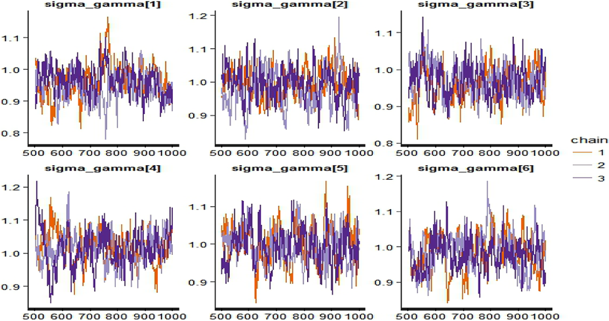
Trace plots of testlet effect parameters in the Rasch testlet model.

Testlet effect parameter estimates in the Rasch testlet model.
Example 3: A Multilevel 3PL IRT Model
This example demonstrates how to fit a multilevel 3PL IRT model in Stan. The data set is an end-of-program learning outcome assessment test for students enrolled in engineering programs in a Middle-Eastern country. The purpose of the analysis is on evaluating those programs based on program mean scores. A traditional approach to computing program mean scores is to calibrate items and score students with an IRT model and average individual scores within a program to obtain the program mean score. However, such an approach ignores the measurement error inherent in individual scores. An alternative, as proposed by Fox and Glas (2001), is to use a multilevel IRT model that simultaneously estimates item parameters, individual scores, and program mean scores. This example fits a 3PL multilevel IRT model that takes into consideration the measurement error in individual scores to estimate program mean scores. The multilevel 3PL IRT model is expressed as follows:

where
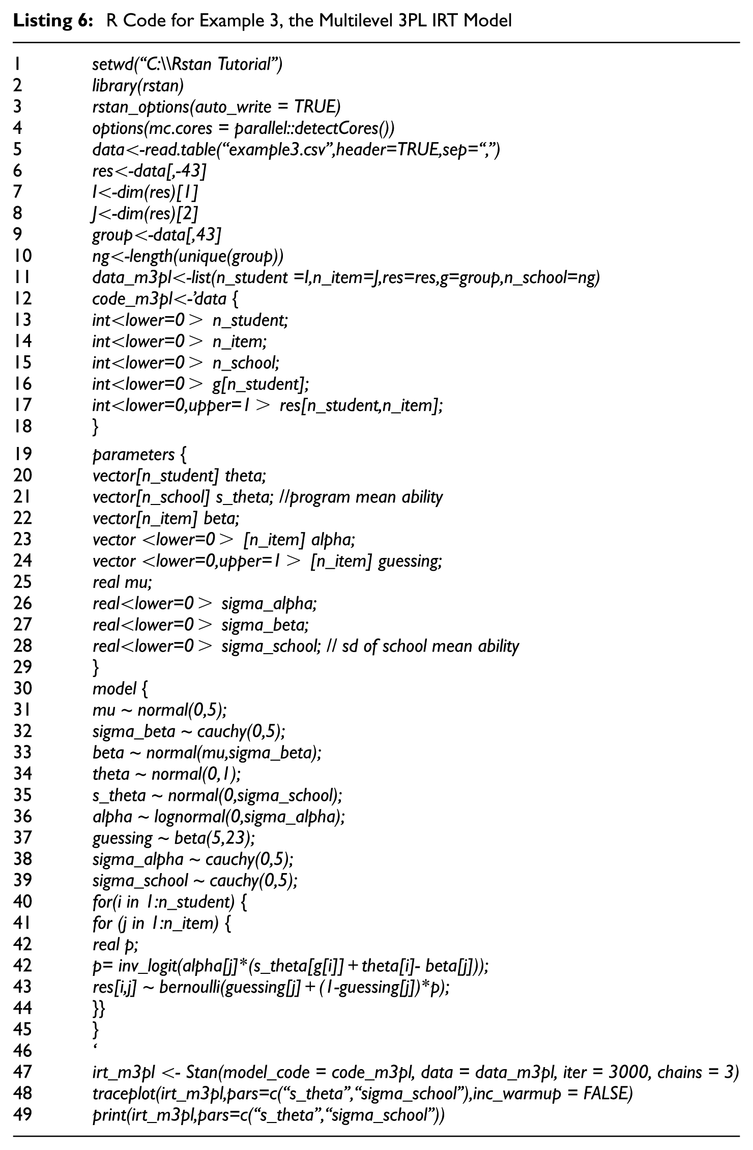
The R code for this example is provided in Listing 6. The data set consists of 43 columns, with the first 42 for item responses and the last one for the group membership for each person. Item responses and the group membership are imported in lines 6 and 9 of Listing 6, and the number of items, examinees, and programs are extracted in lines 7, 8, and 10 of Listing 6. The Stan program for the multilevel 3PL IRT model is defined as an R object named code_m3pl (Listing 6, lines 12-46). To avoid repetition, the illustration of this example focuses on additional Stan codes in Listing 6 related to the multilevel structure.
The group membership information and the number of groups are included in the data block (Listing 6, lines 15-16). In the parameter block, two lines are added for the program mean score parameter (s_theta) and its standard deviation (sigma_school; Listing 6, lines 21 & 28). In the model block, a normal distribution with a mean of 0 and unknown standard deviation (sigma_school) is specified as the prior for s_theta (Listing 6, line 35) whereas a half Cauchy distribution is set as the hyper priors for the parameter sigma_school (Listing 6, line 39). The sampling statement (Listing 6, lines 40-44) in this example is similar to that of the 3PL IRT model (Listing 1, lines 33-37), with the addition of the program mean score parameter s_theta[g[i]]. In this example, a double loop is still used instead of a single loop as the function bernoulli does not allow vectorization for the 3PL model.
For this model, 1,000 iterations are sufficient for convergence. To be conservative, three chains were run with 3,000 iterations for each chain (Listing 6, line 47) and as default, the first 1,500 iterations were discarded as burnin and subsequent inferences were based on the last 1,500 iterations in each chain. The computation took 45 minutes on a desktop computer with an Intel Xeon E5 processor. Based on our experience, BUGS may need tens of thousands of iterations and hours of running time to estimate parameters for this model. Such a noticeable difference in computation time confirms the efficiency of the HMC algorithm implemented in Stan over the traditional MCMC algorithms.
The trace plots for s_theta and sigma_school are requested, as well as the summary statistics of the posterior distributions (Listing 6, lines 48-49). Figures 5 and 6 show the trace plots and the screenshot of the parameter estimates printed in the R console. As can be seen, good mixing is observed for all trace plots in Figure 5, and the PSRF values for all parameters shown in Figure 6 are all below 1.1, with the largest value being 1.02. Though not listed here, all the other model parameters have similar trace plots and PSRF values no greater than 1.05, indicating that convergence has been reached. The 95% credible interval for each s_theta allows to determine whether a particular program has a mean score significantly different from zero (the grand mean score). Take Program 11 as an example: Since s_theta[11] has a posterior mean of 1.67 with a 95% credible interval of (0.90, 2.39), this program has a program effect significantly above the average and is therefore classified as effective. The estimated standard deviation of the program effect is 1.17 with a 95% credible interval of (0.84, 1.67), suggesting that in this data set, there is substantial between-program variation.

Trace plots of program effect parameters in the multilevel three-parameter logistic item response theory (3PL IRT) model.
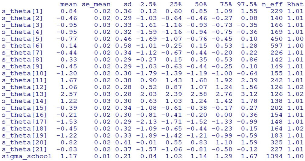
Program effect parameter estimates in the multilevel three-parameter logistic item response theory (3PL IRT) model.
Summary
Stan is a relatively new programming software that implements the powerful HMC algorithm. To date, there is no systematic introduction to using Stan for Bayesian IRT model parameter estimation. This article introduces Stan programs for estimating common dichotomous and polytomous IRT models. Furthermore, it demonstrates IRT model comparison with two R packages
Stan is not without limitations. While WinBUGS can automatically generate values from the posterior predictive distribution for missing response data, Stan treats all missing data as parameters and consequently, a Stan user has to define them in the parameters block or transformed parameters block. With the combination of nonsystematic missing patterns and complex models, such procedures can become tedious and error-prone. Stan also lacks support for sampling discrete parameters, and such parameters need to be marginalized out in order to be estimated in Stan. Although there are some sources such as the Stan User Manual that provide some introduction to how to conduct the marginalization, this procedure may require a substantial amount of coding effort and can be difficult to implement to some applied researchers and practitioners. In the psychometric context, such a disadvantage translates into the fact that mixture IRT models and latent class models cannot be directly specified in Stan, since both contain discrete latent variables. In contrast, BUGS allows for straightforward specifications of such models.
It is hoped that this tutorial will introduce Stan to interested researchers as a powerful and efficient software program suitable for Bayesian IRT analysis. The introduction to the common dichotomous and polytomous IRT models and their multidimensional and multilevel extensions will reduce the learning curve of Stan and facilitate model parameter estimation for further extended IRT models. For researchers who want to fit more complex IRT models to their data using MCMC algorithm but are not satisfied with the computational speed of the Gibbs sampler and Metropolis algorithm in BUGS and other MCMC packages, Stan may be an attractive alternative.
Footnotes
Appendix
R Code for Example 3, the Multilevel 3PL IRT Model
| 1 | setwd(“C:\\Rstan Tutorial”) |
| 2 | library(rstan) |
| 3 | rstan_options(auto_write = TRUE) |
| 4 | options(mc.cores = parallel::detectCores()) |
| 5 | data<-read.table(“example3.csv”,header=TRUE,sep=“,”) |
| 6 | res<-data[,-43] |
| 7 | I<-dim(res)[1] |
| 8 | J<-dim(res)[2] |
| 9 | group<-data[,43] |
| 10 | ng<-length(unique(group)) |
| 11 | data_m3pl<-list(n_student =I,n_item=J,res=res,g=group,n_school=ng) |
| 12 | code_m3pl<-’data { |
| 13 | int<lower=0> n_student; |
| 14 | int<lower=0> n_item; |
| 15 | int<lower=0> n_school; |
| 16 | int<lower=0> g[n_student]; |
| 17 | int<lower=0,upper=1> res[n_student,n_item]; |
| 18 | } |
| 19 | parameters { |
| 20 | vector[n_student] theta; |
| 21 | vector[n_school] s_theta; //program mean ability |
| 22 | vector[n_item] beta; |
| 23 | vector <lower=0> [n_item] alpha; |
| 24 | vector <lower=0,upper=1> [n_item] guessing; |
| 25 | real mu; |
| 26 | real<lower=0> sigma_alpha; |
| 27 | real<lower=0> sigma_beta; |
| 28 | real<lower=0> sigma_school; // sd of school mean ability |
| 29 | } |
| 30 | model { |
| 31 | mu ~ normal(0,5); |
| 32 | sigma_beta ~ cauchy(0,5); |
| 33 | beta ~ normal(mu,sigma_beta); |
| 34 | theta ~ normal(0,1); |
| 35 | s_theta ~ normal(0,sigma_school); |
| 36 | alpha ~ lognormal(0,sigma_alpha); |
| 37 | guessing ~ beta(5,23); |
| 38 | sigma_alpha ~ cauchy(0,5); |
| 39 | sigma_school ~ cauchy(0,5); |
| 40 | for(i in 1:n_student) { |
| 41 | for (j in 1:n_item) { |
| 42 | real p; |
| 42 | p= inv_logit(alpha[j]*(s_theta[g[i]]+theta[i]- beta[j])); |
| 43 | res[i,j] ~ bernoulli(guessing[j]+(1-guessing[j])*p); |
| 44 | }} |
| 45 | } |
| 46 | ‘ |
| 47 | irt_m3pl <- Stan(model_code = code_m3pl, data = data_m3pl, iter = 3000, chains = 3) |
| 48 | traceplot(irt_m3pl,pars=c(“s_theta”,“sigma_school”),inc_warmup = FALSE) |
| 49 | print(irt_m3pl,pars=c(“s_theta”,“sigma_school”)) |
Declaration of Conflicting Interests
The author(s) declared no potential conflicts of interest with respect to the research, authorship, and/or publication of this article.
Funding
The author(s) received no financial support for the research, authorship, and/or publication of this article.