On the Connections Between Item Response Theory and Classical Test Theory: A Note on True Score Evaluation for Polytomous Items via Item Response Modeling

Abstract

This note highlights and illustrates the links between item response theory and classical test theory in the context of polytomous items. An item response modeling procedure is discussed that can be used for point and interval estimation of the individual true score on any item in a measuring instrument or item set following the popular and widely applicable graded response model. The method contributes to the body of research on the relationships between classical test theory and item response theory and is illustrated on empirical data.

Keywords

classical test theory graded response model individual trait level estimate interval estimation item response theory polytomous item true score standard error

The past several decades have seen increased interest in the connections between item response theory (IRT) and item response modeling on one hand, and factor analysis and classical test theory (CTT) on the other (e.g., Takane & de Leeuw, 1987; Zimmerman, 1975; see also Raykov, Dimitrov, Marcoulides, & Harrison, 2017; Raykov & Marcoulides, 2017, and references therein). Their important relationships are highly useful for a deeper understanding of both methodologies and additionally facilitate substantially their well-informed applications. Recently, Raykov et al. (2017) highlighted and illustrated the links between IRT and CTT by discussing an item response modeling procedure for point and interval estimation of the individual true scores on each item in a measuring instrument or set consisting of binary or binary scored measures. The present note extends their procedure to the more general case of homogeneous polytomous items, and is concerned with instruments or item sets following the popular and widely used in educational and behavioral research graded response model (GRM; Samejima, 1969, 2016).

Point and Interval Estimation of Individual True Scores on Ordinal Polytomous Items

Background, Notation, and Assumptions

For the aims of this article, we assume that a set of ordinal polytomous items are given, with each having r response categories that are designated 1, 2, . . ., r (r≥ 2), and note that the following procedure is directly applicable in case of different numbers of responses across items. (The item invariance in these numbers is inconsequential for the method outlined in the sequel, entails no limitation of generality, and is assumed in this discussion merely for the sake of convenience.) We symbolize the items by Y₁, Y₂, . . ., Y_k (k > 1) and presume that they are the components of a considered unidimensional multi-item measuring instrument or item set, such as a psychometric scale or test (referred to as “instrument” below; these may be items that are for instance used in a partial scoring setting or represent the responses on Likert-type questions).¹ We stipulate that the instrument has been administered to a sample of independent subjects from a studied population that is not a mixture of two or more latent classes (cf. Raykov, Marcoulides, & Chang, 2016). Last, we posit that the GRM is valid in the population for these items, and will designate by θ the underlying latent trait or ability (latent dimension) being evaluated by them.

Point Estimation of Item-Specific Individual True Scores

Following CTT, the true score T_ij of the ith examined individual on the jth item is the expectation of his or her pertinent item score (treated as a random variable, at his or her given level of the underlying ability or trait θ as in the rest of this section):

T_{ij} = T_{ij} (θ_{i}) = ε (Y_{ij}),

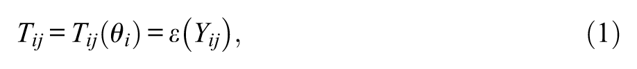
where θ_i is this person’s ability or trait level, Y_ij their observed score on the item, and ε(·) symbolizes expectation with respect to the pertinent propensity distribution of possible item scores (i = 1, . . ., n, with n denoting sample size and j = 1, . . ., k; Lord & Novick, 1968). Since, Y_ij is a discrete random variable, its expectation is (e.g., Casella & Berger, 2002)

ε (Y_{ij}) = 1 \cdot P (Y_{ij} = 1) + 2 \cdot P (Y_{ij} = 2) + \dots + r \cdot P (Y_{ij} = r),

where P(·) denotes probability (and a dot is used to symbolize multiplication, as in the remainder of the section). According to the GRM (cf. de Ayala, 2009),

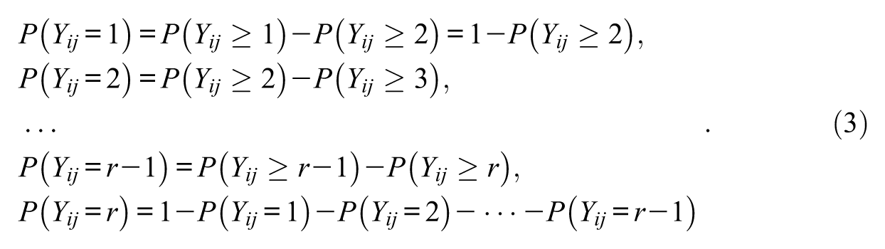
\begin{matrix} P (Y_{ij} = 1) = P (Y_{ij} \geq 1) - P (Y_{ij} \geq 2) = 1 - P (Y_{ij} \geq 2), \\ P (Y_{ij} = 2) = P (Y_{ij} \geq 2) - P (Y_{ij} \geq 3), \\ \dots \\ P (Y_{ij} = r - 1) = P (Y_{ij} \geq r - 1) - P (Y_{ij} \geq r), \\ P (Y_{ij} = r) = 1 - P (Y_{ij} = 1) - P (Y_{ij} = 2) - \dots - P (Y_{ij} = r - 1) \end{matrix} .

In Equations (3), P(Y_ij≥m) are the probabilities of responding in category m or higher, which are of main modeling interest and are parameterized in the GRM as follows:

P (Y_{ij} \geq m) = 1 / {1 + \exp [- a_{j} (θ_{i} - b_{jm})]},

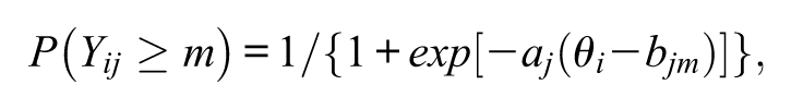
with exp(·) denoting exponentiation, a_j an item discrimination parameter, and b_jm a cut-point that can be thought of as a difficulty parameter associated with a response in category m or higher (m = 2, 3, . . ., r). That is, these probabilities can be viewed as formally satisfying the two-parameter logistic model with an item-specific discrimination parameter and r−1 additional parameters associated each with the corresponding ordered category of the item (second through last), whereby P(Y_ij > r) = 0 is presumed (“Stata Item Response Theory Manual,” 2015; cf. Samejima, 1969, 2016). In the rest of the article, for simplicity of reference the latter r−1 quantities are called “item difficulty parameters.”

Hence, from Equations (1) through (3) it follows that the true score of the ith individual on the jth item is (cf. de Ayala, 2009)

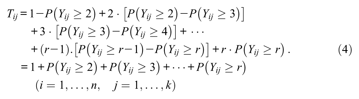
\begin{matrix} T_{ij} = 1 - P (Y_{ij} \geq 2) + 2 \cdot [P (Y_{ij} \geq 2) - P (Y_{ij} \geq 3)] \\ + 3 \cdot [P (Y_{ij} \geq 3) - P (Y_{ij} \geq 4)] + \dots \\ + (r - 1) . [P (Y_{ij} \geq r - 1) - P (Y_{ij} \geq r)] + r \cdot P (Y_{ij} \geq r) \\ = 1 + P (Y_{ij} \geq 2) + P (Y_{ij} \geq 3) + \dots + P (Y_{ij} \geq r) \\ (i = 1, \dots, n, j = 1, \dots, k) \end{matrix} .

Therefore, after fitting the GRM to a given data set on ordinal polytomous items (and finding it plausible), the point estimates of the individual true scores on any of the k items under consideration are obtainable from Equation (3) as

{\hat{T}}_{ij} = 1 + \hat{P} (Y_{ij} \geq 2) + \hat{P} (Y_{ij} \geq 3) + \dots + \hat{P} (Y_{ij} \geq r),

where a hat is used to denote estimate of the quantity underneath, as in the remainder of this note, and $\hat{P}$ (.) denotes the model-based estimated probability of the event following in parentheses (i = 1, . . ., n, j = 1, . . ., k).²

Interval Estimation of Item-Specific Individual True Scores

Equation (5) only provides point estimates of the individual persons’ true scores on any item in an instrument or item set under consideration, with no information regarding the instability of these estimates. To resolve this issue, all estimated item discrimination and difficulty parameters are treated next as known, for instance, from prior calibration or application of the marginal maximum likelihood estimation method (e.g., Reckase, 2009; see also Raykov et al., 2017), as is nearly routinely proceeded with in corresponding IRT applications. In this way, by utilizing the delta method (e.g., Raykov & Marcoulides, 2004), we can furnish the following approximate standard error (SE) for the item-specific, individual true score in Equation (5) (cf. Raykov et al., 2017):

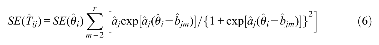
SE ({\hat{T}}_{ij}) = SE ({\hat{θ}}_{i}) \sum_{m = 2}^{r} [{\hat{a}}_{j} \exp [{\hat{a}}_{j} ({\hat{θ}}_{i} - {\hat{b}}_{jm})] / {1 + \exp [{\hat{a}}_{j} ({\hat{θ}}_{i} - {\hat{b}}_{jm})]}^{2}],

(i = 1, . . ., n, j = 1, . . ., k). (A standard error appearing in Equation 6 is by definition the positive square root of the pertinent approximate variance resulting from the delta method; e.g., Casella & Berger, 2002.)

Employing the standard error in Equation (6) and the true score estimate in Equation (5) with the monotone transformation-based procedure using the logistic function in Raykov and Marcoulides (2011, chapter 7; after a suitable initial linear transformation, see below and Appendix B), we finally obtain for each person and item a confidence interval (CI) of his or her true score on the jth item:

(T_{ij, lo} (α), T_{ij, up} (α)),

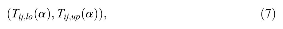
where T_ij,lo(α) and T_ij,up(α), respectively, denote the lower and upper limit of the 100(1 −α)% CI for the true score of the ith examined person on the item (0 < α < 1; i = 1, . . ., n, j = 1, . . ., k).

The item-specific individual true score estimate in Equation (5) as well as its associated standard error in Equation (6) and CI in (7) are readily obtained using widely circulated statistical software, such as Stata and R (e.g., Raykov & Marcoulides, 2017; see also the Mplus source code for examining the plausibility of the GRM, which is provided in appendix 1 of Raykov et al., 2017). The source code needed for the point estimation of the item-specific individual true scores and the associated approximate standard error (Equations 5 and 6) is supplied in Appendix A to this note, and the R-function for the construction of the true score CI (7) is found in Appendix B.

The applicability and utility of the discussed true score estimation procedure is demonstrated next on empirical data.

Illustration on Data

For the purposes of this section, we make use of a data set from an anxiety study that is available with a download from www.ssicentral.com of the (student version of the) IRT software IRTPRO (Cai, Thissen, & du Toit, 2017). The data set results from k = 5 ordinal polytomous items with r = 5 response options each that were administered to n = 514 persons and asked about their feelings of being calm, at ease, tense, regretful, or nervous (e.g., du Toit, 2003). For the sake of illustration and ease of reference, the aims of the present discussion, and without loss of generality these items might be thought of in the remainder as being possibly indicative of the trait Generalized Anxiety.

We commence by examining the plausibility of the GRM. To this end, as in Raykov et al. (2017), we use confirmatory factor analysis for the five categorical items and apply the popular latent variable modeling software Mplus for fitting the pertinent single-factor model to them (L. K. Muthén & Muthén, 2017; see appendix 1 in Raykov et al., 2017, for the needed source code and notes to it). The overall goodness-of-fit indices of the GRM fitted thereby are nonsignificant and suggest that it is a tenable means of data description and explanation: Pearson chi-square value = 1682.251, degrees of freedom (df) = 3090, associated p value (p) = 1; and likelihood ratio chi-square value = 837.822, df = 3090, p = 1.³ In addition, the individual item R ² indices range between 32% and 71%, and thus none of them can be seen as indicating potentially serious “local” violations of model fit. With these global and “local” goodness-of-fit results, we may conclude that the GRM is plausible for the analyzed data set.

Next, we obtain the point estimates of the individual Generalized Anxiety trait levels, that is, the above values ${\hat{θ}}_{i}$ (i = 1, . . ., n, with n = 514 here; see Appendix A for the needed Stata source code). This is achieved with the first couple of commands in the Stata source code in Appendix A (after the initial three comment lines). With these latent trait estimates as well as the item discrimination and difficulty parameter estimates (i.e., of a_j and b_jm; j = 1, . . ., 5, m = 2, . . ., 5), using Equation (5), we arrive at the point estimates of the 514 individual true scores on each of the five items. This is accomplished with the next four lines in the Stata code in Appendix A (after the pertinent comment line). The resulting true score estimates for the first 10 subjects say are presented in Table 1.

Table 1.

Individual True Score Estimates on Each of k = 5 Anxiety Items (for the First 10 Subjects, in Stata Format).

	calm	at ease	tense	regretful	nervous	T1	T2	T3	T4	T5
1	3	3	2	2	2	2.493538	2.678101	2.651873	2.357293	2.530299
2	3	3	5	5	3	3.231783	3.420408	3.455674	2.983735	3.236365
3	3	3	3	3	4	2.925919	3.10302	3.120781	2.714475	2.937812
4	3	3	2	2	3	2.600281	2.784837	2.764364	2.441504	2.627367
5	2	3	2	4	4	2.560339	2.745312	2.722132	2.409815	2.590901
6	1	1	1	1	2	1.173661	1.254172	1.288422	1.370501	1.370685
7	3	2	1	1	1	1.782303	1.944211	1.901951	1.797227	1.874782
8	1	1	2	1	1	1.236826	1.343809	1.362768	1.424015	1.432933
9	3	3	3	1	1	2.510716	2.695529	2.669911	2.370757	2.545853
10	3	2	2	1	1	1.994575	2.149248	2.120625	1.959929	2.066717

Note. Tj = individual true score on the jth item (j = 1, . . ., 5, in the order “calm,”“atease,”“tense,”“regretful,” and “nervous”; subject identifier given in left-most column).

In the second step of the procedure of this article, employing these individual true score estimates and based on Equation (6), we furnish the standard errors associated with each of the 514 individual true scores (estimates) on any of the five items. This is accomplished with the following nine lines in the Stata code in Appendix A (after the pertinent comment line). These standard errors for the first 10 respondents are presented in Table 2.

Table 2.

Standard Errors for the Individual True Score Estimates in Table 1 (for the First 10 Subjects, in Stata Format).

	T1	T1_SE	T2	T2_SE	T3	T3_SE	T4	T4_SE	T5	T5_SE
1	2.493538	0.313361	2.678101	0.3188743	2.651873	0.3289223	2.357293	0.2454092	2.530299	0.2836159
2	3.231783	0.3380273	3.420408	0.3509775	3.455674	0.3496579	2.983735	0.2905437	3.236365	0.31761
3	2.925919	0.2866951	3.10302	0.2878803	3.120781	0.3222451	2.714475	0.2521445	2.937812	0.2833688
4	2.600281	0.3114646	2.784837	0.3065315	2.764364	0.330206	2.441504	0.248196	2.627367	0.2852975
5	2.560339	0.3329757	2.745312	0.3314064	2.722132	0.351201	2.409815	0.2631197	2.590901	0.3030938
6	1.173661	0.17563	1.254172	0.2554093	1.288422	0.2167151	1.370501	0.1608515	1.370685	0.1859264
7	1.782303	0.3271973	1.944211	0.307346	1.901951	0.3244133	1.797227	0.2368114	1.874782	0.2802187
8	1.236826	0.2116557	1.343809	0.2925058	1.362768	0.2386862	1.424015	0.16746	1.432933	0.1958754
9	2.510716	0.3258688	2.695529	0.3296319	2.669911	0.342316	2.370757	0.255632	2.545853	0.2951923
10	1.994575	0.2961472	2.149248	0.2995908	2.120625	0.315244	1.959929	0.2372342	2.066717	0.2789896

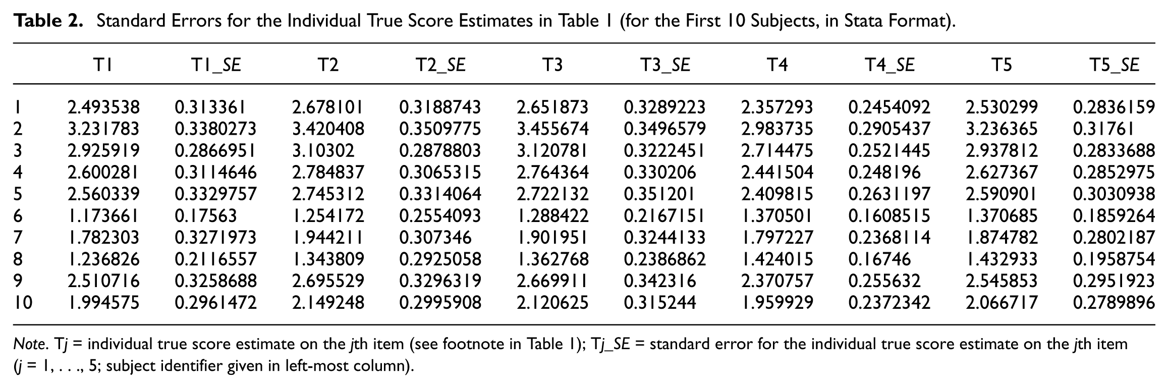
Note. Tj = individual true score estimate on the jth item (see footnote in Table 1); Tj_SE = standard error for the individual true score estimate on the jth item (j = 1, . . ., 5; subject identifier given in left-most column).

In the third step of the method discussed in this note, utilizing the R-function “ci.ordinal_polytomous_item_TS” in Appendix B with the true score estimates and their standard errors obtained as above, we finally furnish the 95% CIs for each of the 514 individual true scores on any of the five items. These CIs for the first 10 persons and first item are presented in Table 3.

Table 3.

Confidence Intervals at 95% Confidence Level for the Individual True Scores (for First 10 Subjects and First Item, “Calm,” in Stata Format).

id	T1	T1_SE	T1_low	T1_up
1	2.493538	0.3133610	1.944534	3.138326
2	3.231783	0.3380273	2.568180	3.847397
3	2.925919	0.2866951	2.383873	3.479087
4	2.600281	0.3114646	2.043796	3.229680
5	2.560339	0.3329757	1.974632	3.237688
6	1.173661	0.17563	1.022728	2.059820
7	1.782303	0.3271973	1.322688	2.609956
8	1.236826	0.2116557	1.038733	2.153108
9	2.510716	0.3258688	1.941091	3.179467
10	1.994575	0.2961472	1.528359	2.673828

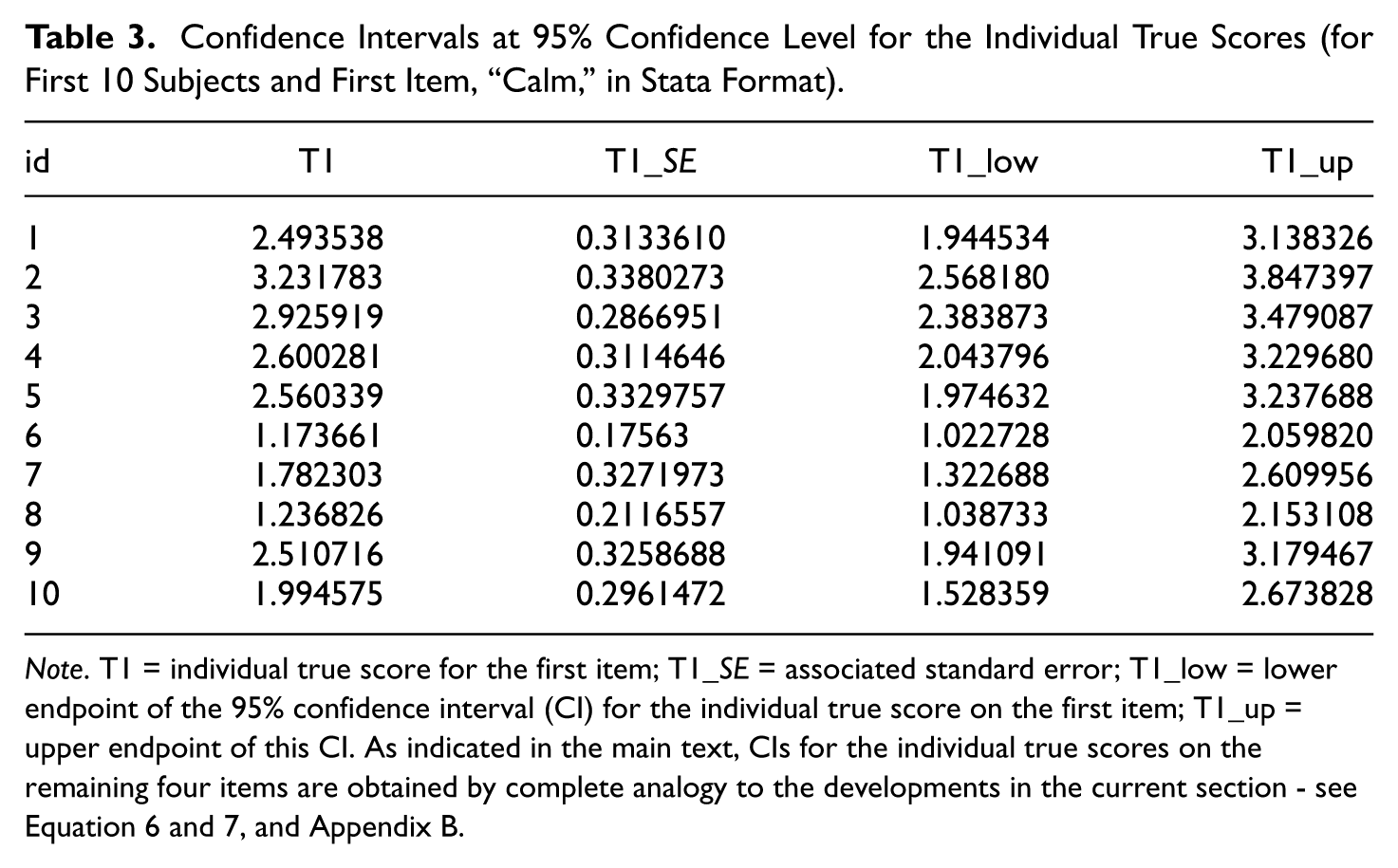
Note. T1 = individual true score for the first item; T1_SE = associated standard error; T1_low = lower endpoint of the 95% confidence interval (CI) for the individual true score on the first item; T1_up = upper endpoint of this CI. As indicated in the main text, CIs for the individual true scores on the remaining four items are obtained by complete analogy to the developments in the current section - see Equation 6 and 7, and Appendix B.

The individual true score CIs with respect to the remaining four items are obtained by complete analogy, using their earlier rendered true score estimates and associated standard errors.

Conclusion

In this note, we have discussed an extension of the true score point and interval estimation procedure in Raykov et al. (2017) to the case of ordinal polytomous items. The method has generalized their procedure to the setting of a unidimensional measuring instrument or item set adhering to the popular and widely applicable GRM, with that earlier procedure being a special case of the present one (when r = 2). We were similarly concerned here with an IRT modeling–based approach to point and interval estimation of individual true scores on each item in an item set under consideration that followed the GRM, and our goal was also to highlight and illustrate further important and useful links between IRT and CTT.

It is worthwhile stressing at this point several limitations of the estimation approach of the present article. One is the requirement of large samples with respect to both persons and items, since it is instrumentally based on maximum likelihood estimation that is grounded in an asymptotic theory (see Raykov et al., 2017, for additional discussion on this general limitation, in particular with respect to number of items). Two, the discussed method rests on the assumption of the items following the GRM, and therefore, its application with an instrument or item set that is multidimensional is not recommendable (cf. Reckase, 2009). Three, we have assumed that the instrument or considered items are given, that is, prespecified, rather than sampled from a pool, population, or universe of items. Last, the procedure of this note makes extensive use of the delta method that is based on a linear approximation, and it is unknown to what extent its approximate validity may be generalizable to complex parametric functions representing expected observed scores (true scores) in models other than the GRM.

In conclusion, this note provides educational and behavioral scientists with a widely applicable procedure for estimation of individual true scores on any of the items in a unidimensional measuring instrument or item set adhering to the popular GRM, and contributes further to the body of research on the connections between IRT and CTT (e.g., Raykov et al., 2017, and references therein).

Footnotes

Appendix A

Appendix B

Acknowledgements

We are grateful to B. Muthén and L. Steinberg for valuable discussions on the graded response model. We are indebted to R. Raciborski for helpful and instructive comments on applications of the Stata IRT module.

Declaration of Conflicting Interests

The author(s) declared no potential conflicts of interest with respect to the research, authorship, and/or publication of this article.

Funding

The author(s) received no financial support for the research, authorship, and/or publication of this article.

Notes

References

Cai

Thissen

du Toit

S. H. C.

(2017). IRTPRO 4.1 for Windows [Computer software]. Skokie, IL: Scientific Software International.

Casella

Berger

(2002). Statistical inference. Monterey, CA: Wadsworth.

de Ayala

R. J

. (2009). The theory and practice of item response theory. New York, NY: Guilford Press.

du Toit

. (Ed.). (2003). IRT from SSI. Skokie, IL: Scientific Software International.

Lord

F. M.

Novick

M. R.

(1968). Statistical theories of mental test scores. Reading, MA: Addison-Wesley.

Muthén

L. K.

Muthén

B. O.

(2017). Mplus user’s guide. Los Angeles, CA: Muthén & Muthén.

Raykov

Dimitrov

D. M.

Marcoulides

G. A.

Harrison

(2017). On true score evaluation using item response theory modeling. Educational and Psychological Measurement, 79, 796-807. doi:10.1177/0013164417741711

Raykov

Marcoulides

G. A.

(2004). Using the delta method for approximate interval estimation of parametric functions in covariance structure models. Structural Equation Modeling, 11, 659-675.

Raykov

Marcoulides

G. A.

(2011). Introduction to psychometric theory. New York, NY: Taylor & Francis.

10.

Raykov

Marcoulides

G. A.

(2017). A course in item response theory and modeling with Stata. College Station, TX: Stata Press.

11.

Raykov

Marcoulides

G. A.

Chang

(2016). Studying population heterogeneity in finite mixture settings using latent variable modeling. Structural Equation Modeling, 23, 726-730.

12.

Reckase

M. D.

(2009). Multidimensional item response theory. New York, NY: Springer.

13.

Samejima

(1969). Estimation of latent ability using a response pattern of graded scores (Psychometrika Monograph No. 17). Richmond, VA: Psychometric Press.

14.

Samejima

(2016). Graded response models. In van der Linden

W. J.

(Ed.), Handbook of item response theory (Vol. 1, pp. 95-108). Boca Raton, FL: CRC Press.

15.

Stata Item Response Theory Manual: Release 14. (2015). College Station, TX: Stata Press.

16.

Takane

de Leeuw

(1987). On the relationship between item response theory and factor analysis of discretized variables. Psychometrika, 52, 393-408.

17.

von Davier

. (2016). Rasch model. In van der Linden

W. J.

(Ed.), Handbook of item response theory (Vol. 1, pp. 31-50). Boca Raton, FL: CRC Press.

18.

Zimmerman

D. W.

(1975). Probability spaces, Hilbert spaces, and the axioms of test theory. Psychometrika, 40, 395-412.