
Abstract
We examine the accuracy of p values obtained using the asymptotic mean and variance (MV) correction to the distribution of the sample standardized root mean squared residual (SRMR) proposed by Maydeu-Olivares to assess the exact fit of SEM models. In a simulation study, we found that under normality, the MV-corrected SRMR statistic provides reasonably accurate Type I errors even in small samples and for large models, clearly outperforming the current standard, that is, the likelihood ratio (LR) test. When data shows excess kurtosis, MV-corrected SRMR p values are only accurate in small models (p = 10), or in medium-sized models (p = 30) if no skewness is present and sample sizes are at least 500. Overall, when data are not normal, the MV-corrected LR test seems to outperform the MV-corrected SRMR. We elaborate on these findings by showing that the asymptotic approximation to the mean of the SRMR sampling distribution is quite accurate, while the asymptotic approximation to the standard deviation is not.
Structural equation modeling (SEM) is a popular technique for modeling multivariate data because it provides a comprehensive framework for fitting theoretical models. Given that SEM is most often used for furthering theory development, a substantial body of literature to date has focused on the issue of how to assess model–data fit (i.e., goodness of fit) in SEM. There appear to be two general perspectives with regard to goodness of fit in SEM. One perspective revolves around the notion that one should not expect to find and thus not seek a model that may be considered as precisely true or correct in the population (e.g., MacCallumet al., 1992). From this perspective, applied researchers should aim at showing that a model provides a good approximation to real-world phenomena, as represented in an observed set of data. To do so, it is generally recommended that multiple approaches to assessment of fit be used (MacCallum, 1990). These may be purely descriptive, involving a comparison of the fitted model to another model, such as a saturated model, or to independence model (Bentler & Bonett, 1980). This perspective appears to be frequently employed, for instance, when fitting exploratory factor analysis models (Lim & Jahng, 2019). From this perspective, assessing whether the model fits the data exactly appears almost unnecessary.
The alternative perspective is concerned with the quality of inferences drawn using the fitted model. From this perspective, assessing the exact fit of a model is important because, provided that alternative equivalent models (Bentler & Satorra, 2010; MacCallum et al., 1993; Stelzl, 1986) can be ruled out theoretically and that the power of the test (Lee et al., 2012; Saris & Satorra, 1993) is sufficiently large, failing to reject the null hypothesis of exact fit enables drawing statistical inferences on the parameter estimates (Bollen & Pearl, 2013; Maydeu-Olivares et al., 2020). Of course, as sample size increases the power to reject the hypothesis of exact model fit increases (Jöreskog, 1967). Also, as model size increases it becomes increasingly difficult to find a well-fitting model, simply due to time constraints (Maydeu-Olivares, 2017a). From this perspective, assessing the exact fit of a model is a meaningful endeavor, always coupled with an assessment of the size of model misfit, with confidence intervals (Maydeu-Olivares, 2017a; Steiger, 1989).
Because sample goodness-of-fit indices are estimators of population quantities, both perspectives can be integrated by using confidence intervals (and if of interest, significance tests) for population effect sizes of misfit. Confidence intervals for the root mean squared error of approximation (RMSEA; Steiger & Lind, 1980; see also Browne & Cudeck, 1993) are well known and routinely used in applications. Steiger (1989) showed that it is possible to obtain confidence intervals for the population goodness-of-fit index (GFI; Jöreskog & Sörbom, 1988; see also MacCallum & Hong, 1997; Maiti & Mukherjee, 1990; Tanaka & Huba, 1985). The sampling distribution of the comparative fit index (CFI; Bentler, 1990) may also be approximated using asymptotic methods (Lai, 2019). Finally, confidence intervals for the standardized root mean squared residual (SRMR; Bentler, 1995) can be obtained using a normal distribution (Maydeu-Olivares, 2017a; Maydeu-Olivares et al., 2018; Ogasawara, 2001). Therefore, if the purpose of the analysis is simply to provide an approximate representation of the phenomena under investigation, confidence intervals for any of these estimands should be obtained. It is important to use unbiased estimators of the estimands of interest as well as confidence intervals because at small to moderate sample sizes the sample goodness-of-fit indices commonly used in applications can be severely biased and may display a large sampling variability (Maydeu-Olivares et al., 2018; Shi et al., 2019; Steiger, 1990). On the other hand, if the purpose of the analysis is to draw causal inferences on the model parameters, then it makes more sense to test whether the population value of these effect sizes suggests a perfect fit.
The only effect size of model misfit that is currently used in applications is the RMSEA. Put differently, the RMSEA is the only goodness-of-fit index for which SEM software routinely provide a p value for a test of close fit. The null and alternative hypotheses can be written as

where N denotes sample size,
When data are not normal, the most widely used test statistic is the likelihood ratio test statistic, either scaled by its asymptotic mean or adjusted by its asymptotic mean and variance as proposed by Satorra and Bentler (1994). When any of these chi-squares robust to nonnormality is used, (1) is replaced by

where
Recently, Maydeu-Olivares (2017a) introduced a framework for assessing the size of model misfit using the SRMR. Confidence intervals and, if of interest, tests of close fit can now be performed using the SRMR in addition to the RMSEA. Extant research (Maydeu-Olivares et al., 2018; Shi et al., 2020) has shown that more accurate confidence intervals and test of close fit are obtained using the SRMR than the RMSEA. The latter only provides accurate results in small models.
Maydeu-Olivares (2017a) also provided theory for utilizing the SRMR as a test of exact fit, both under normality assumptions and when data are not normal. In a simulation study, involving a confirmatory factor analysis (CFA) model and sample sizes (N) ranging from 100 to 3,000 observations, the author showed that the SRMR p values were accurate even when the smallest sample sizes were considered. Nevertheless, this simulation study relied on a CFA population model involving only eight variables (p = 8) and normally distributed data. In the literature to date, however, it has been repeatedly found that the performance of goodness-of-fit tests worsens as the model size (i.e., the number of variables being modeled) increases (Herzog et al., 2007; Maydeu-Olivares, 2017b; Moshagen, 2012; Shi, Lee, & Terry, 2018; Yuan et al., 2015) and with violations of the normality assumptions (e.g., Hu et al., 1992; Satorra, 1990).
In the current article, we address this gap in the literature and examine whether the SRMR test of exact fit yields accurate p values in a wider range of conditions, involving models of various sizes and both normal and nonnormal data. In addition, we pit the performance of the SRMR against the gold standard for the exact goodness-of-fit assessment, the likelihood ratio test (e.g., Jöreskog, 1969). In the SEM literature, this test statistic is commonly referred to as the chi-square test. In the comparison, we also include the robust, that is, the mean and variance adjusted, chi-square test statistic appropriate for nonnormal data (Asparouhov & Muthén, 2010; Satorra & Bentler, 1994). The remainder of this article is organized as follows. First, we summarize the existing statistical theory for the SRMR. Next, we describe the simulation study conducted to evaluate the accuracy of the asymptotic approximations to the finite sampling distribution of these test statistics. We then summarize the results and provide a discussion of our findings.
The Standardized Root Mean Squared Residual
The Sample SRMR
Let the standardized residual variances and covariances be

where

where
Equation (4) is the SRMR expression computed by the widely used software program LISREL (Jöreskog & Sörbom, 2017) and EQS (Bentler, 2004). It is suitable for assessing how well the assumed (theorized) model reproduces the observed associations among the variables in an interpretable manner. Roughly, it can be interpreted as the average of the absolute value of residual correlations.
On the other hand, the SRMR computed by default in Mplus software (Muthén & Muthén, 2017) is somewhat different:


where mi and
Confidence Intervals for the Population SRMR
The sample SRMR provided in Equation (4) is an estimator of the population SRMR:

Here, σ
ij
denotes the true and unknown population covariance between variables i and j (or variance if i = j) and
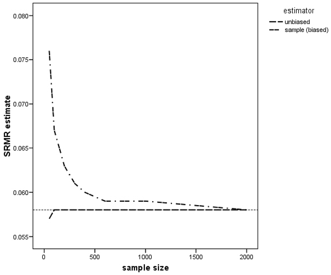
Average sample (i.e., biased) standardized root mean squared residual (SRMR) and unbiased SRMR estimates of the population SRMR of .058 across 1,000 replications as a function of sample size.
In Figure 1, we have also plotted the results of Shi, Maydeu-Olivares, and DiStefano (2018, Table 2) for the average unbiased estimator of the SRMR proposed by Maydeu-Olivares (2017a). As the figure reveals, the unbiased estimator of the SRMR is essentially unbiased for sample sizes over 100 observations. The unbiased estimator of the population SRMR proposed by Maydeu-Olivares (2017a) is
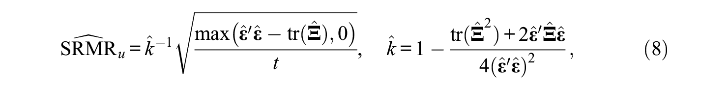
where
Maydeu-Olivares (2017a) proposed using a normal distribution as reference for obtaining confidence intervals and tests of close fit for the population SRMR using the unbiased SRMR estimator. Using this reference distribution, a (100 −α)% confidence interval for the population SRMR, can be obtained with

where

Finally, p values for a null hypothesis of close fit,

where
In needs to be noted that, in principle, these procedures could also be used to test whether a hypothesized SEM model fits exactly. In practice, when the population SRMR equals zero, often
Testing for Exact Fit Using the SRMR
In SEM models without the mean structure, the null and alternative hypotheses of exact fit are generally written as:
Maydeu-Olivares (2017a) has proposed an additional test of the exact fit of the model based on the SRMR. The author showed that under the null hypothesis of exact model fit, the mean and standard error of the sample SRMR in (4) can be approximated in large samples using


Then, the sample SRMR can be used to obtain p values for the null hypothesis of exact fit using

To investigate the performance of the method above, Maydeu-Olivares (2017a) performed a simulation study involving a CFA model with eight observed variables (p = 8), sample sizes (N) ranging from 100 to 3,000, and normally distributed data. The results revealed that the proposed method provided accurate Type I error rates regardless of the sample size and significance level. Nevertheless, it has been repeatedly found in the literature that the performance of goodness-of-fit tests worsens as model size (i.e., the number of variables being modeled) increases (e.g., Herzog et al., 2007; Maydeu-Olivares, 2017b; Moshagen, 2012; Shi, Lee, & Terry 2018; Yuan et al., 2015). Because the initial evidence on the performance of SRMR was limited to a very small model, it seemed necessary to evaluate the performance of this test statistic also in large models. In addition, the SRMR proposal to assess the exact fit of SEM models was evaluated only in the case of normally distributed data (Maydeu-Olivares, 2017a). However, it has been well documented in the literature that the goodness-of-fit tests (e.g., the likelihood ratio test) fail when data are not normal (e.g., Hu et al., 1992; Satorra, 1990). Accordingly, it seemed warranted to evaluate the performance of the exact fit SRMR proposal also in the case of nonnormal data.
Method
We performed a simulation study to examine the performance of SRMR p values to assess the exact fit of SEM models as introduced by Maydeu-Olivares (2017a). The model used to generate the data was a CFA model because it is the most widely used SEM model in empirical research (DiStefano et al., 2018). The population and fitted models were a one-factor model. We used this simple model because the main aim of the study was to investigate the performance of SRMR p values under nonnormality and large model size. The population values for all factor loadings were set to be .70, and all residual variances were set to .51.
Data Generation
Data were generated as follows. Using this population CFA model, we first generated continuous data from a multivariate normal distribution. The continuous data were then discretized into seven categories coded 0 to 6. Methodological studies have shown that when the number of response categories is large (i.e., seven), it is appropriate to treat the discretized data as continuous when fitting CFA models (DiStefano & Morgan, 2014; Rhemtulla et al., 2012). Furthermore, we used discretized normal data because in CFA studies it is more common to model discrete ordinal data (i.e., responses to Likert-type items) than continuous data proper (i.e., test scores). Finally, categorizing continuous variables is employed as a widely used method to generate nonnormally distributed data (DiStefano & Morgan, 2014; Maydeu-Olivares, 2017b; Muthén & Kaplan, 1985).
Study Conditions
The simulation conditions were obtained by manipulating the following three factors: (a) sample size, (b) model size, and (c) level of nonnormality.
Sample Size
Sample sizes included 100, 200, 500, and 1,000 observations. The sample sizes were selected to reflect a range of small to large samples commonly used in psychological research.
Model Size
Model size refers to the total number of observed variables, p (Moshagen, 2012; Shi, Lee, & Terry, 2018). We used three different levels for the number of observed variables: small (p = 10), medium (p = 30), and large (p = 60) models.
Level of Nonnormality
Three levels of nonnormality were obtained by manipulating the population values of the skewness and (excess) kurtosis: (a) skewness = 0.00, kurtosis = 0.00 (i.e., normal data), (b) skewness = 0.00, kurtosis = 3.30, and (c) skewness = −2.00, kurtosis = 3.30. To achieve the designed skewness and kurtosis, the continuous data were discretized using selected threshold values (Maydeu-Olivares, 2017b; Muthén & Kaplan, 1985). The threshold values used for data generation and the expected area under the curve for each response category are presented in Table 1. The technical details for computing the population skewness and kurtosis given a set of thresholds can be found in Maydeu-Olivares et al. (2007).
Target Item Category Probabilities and Corresponding Threshold Values Used to Generate the Data.

In sum, the simulation study consisted of a fully crossed design including four sample sizes, three distributional shapes, and three model sizes. Thirty-six conditions were created in total (4 × 3 × 3). For each of the 36 simulated conditions, 1,000 replications were generated with the simsem package in R (Pornprasertmanit et al., 2013; R Core Team, 2019).
Estimation
For each simulated data set, we fitted a one-factor CFA model with the maximum likelihood estimation method using the lavaan package in R (Rosseel, 2012). In the supplementary materials to this article, we provide R code for computing the exact fit test using SRMR. The SRMR test statistic Equation (14) was obtained under both NT and ADF) assumptions. Different values of this statistic based on the SRMR to assess the exact fit of the model are obtained under NT and ADF assumptions because the asymptotic covariance matrix of the standardized residual covariances, Ξ is computed differently. For computational details of the two SRMR test statistics the reader is referred to Maydeu-Olivares (2017a).
To benchmark the performance of the SRMR as a test of exact fit, we used the likelihood ratio (Jöreskog, 1969) test, also commonly known as the chi-square test (χ2). The chi-square test statistic was also obtained both NT and ADF assumptions. The χ2 statistic computed under normality is the likelihood ratio test. The χ2 statistic computed under ADF is the mean and variance adjusted likelihood ratio test statistic proposed by Asparouhov and Muthén (2010; see also Satorra & Bentler, 1994). For both χ2 and SRMR statistics, we evaluated the empirical rejection rates, that is, Type I error rates using nominal alpha levels of 5%.
Results
For all the study conditions all replications successfully converged. Accordingly, results for each of the 36 conditions under investigation were based on all 1,000 replications.
We provide in Table 2 the empirical rejection rates at the 5% significance level of the χ2 and SRMR tests of exact fit. Following Bradley (1978), and taking into account that we used only 1,000 replications, we considered Type I error rates in [.02, .08] to be adequate. Conditions that fall outside this range are highlighted in Table 2.
Empirical Rejection Rates at the 5% Significance Level of the Chi-Square and SRMR Tests of Exact Fit.
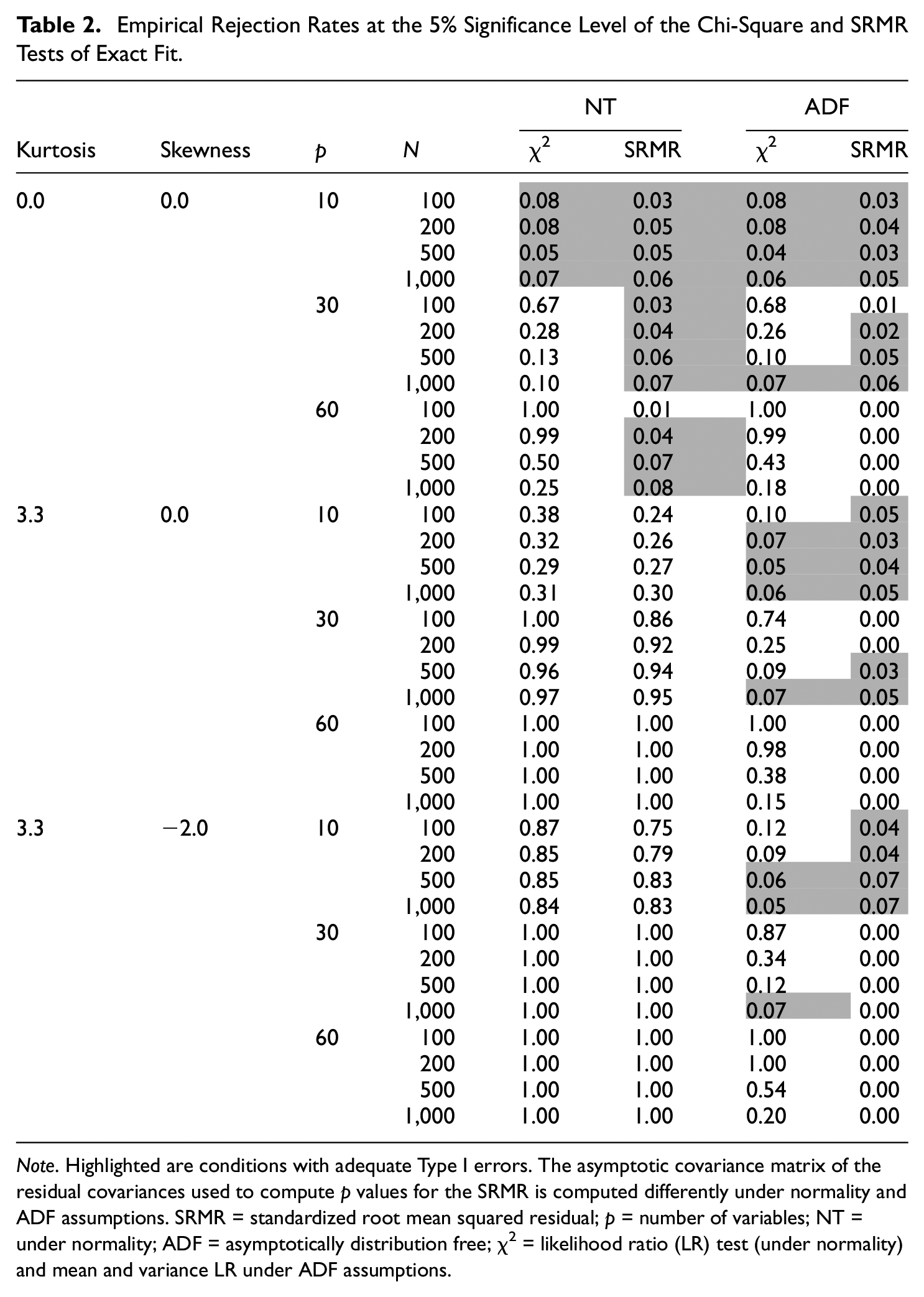

Note. Highlighted are conditions with adequate Type I errors. The asymptotic covariance matrix of the residual covariances used to compute p values for the SRMR is computed differently under normality and ADF assumptions. SRMR = standardized root mean squared residual; p = number of variables; NT = under normality; ADF = asymptotically distribution free; χ2 = likelihood ratio (LR) test (under normality) and mean and variance LR under ADF assumptions.
The results presented in Table 2 for the χ2 statistic were consistent with previous findings in the literature. Specifically, the χ2 computed under normality assumption (NT in the table) overrejected the true model when data were nonnormal. Furthermore, the rejection rates increased as the model size increased. For the nonnormal conditions investigated, as soon as p = 30, the test almost always rejected the model. In fact, the only conditions investigated for which the test maintained adequate Type I error rates involved normal data and a small model (p = 10). For normal data and larger models (p≥ 30), the NT χ2 statistic converged slowly to its asymptotic distribution, but even the largest sample size considered (1,000) was insufficient to obtain accurate Type I error rates.
We also see in Table 2 that with the increasing number of variables, the robust χ2 (ADF in the table) converged faster than the NT χ2 to its reference distribution, that is, it was more robust to the model size effect. This is consistent with previous findings in the literature (e.g., Maydeu-Olivares, 2017b). Under normality, the robust χ2 achieved adequate Type I errors when p = 30 with 1,000 observations. However, sample sizes larger than 1,000 are needed for this statistic to yield accurate Type I error rates when p = 60. As expected, the ADF χ2 was also more robust to the effect of nonnormality. Specifically, p values were acceptable for p = 10 and the minimum sample size needed to achieve them varied depending on the level of kurtosis and skewness in the data. A minimum of 100 observations was needed when the data shows neither (excess) kurtosis nor skewness (i.e., normal data), 200 observations when the data showed only excess kurtosis, and of 500 observations when both kurtosis and skewness were present. For p = 30, larger sample sizes (i.e., 1,000 observations) were needed for the test to yield nominal Type I error rates. Finally, for p = 60, not even the largest sample sizes (i.e., 1,000) were sufficient to obtain accurate Type I error rates.
Results for the test of exact fit using the SRMR revealed a pattern different from the one observed for the χ2 test statistic. When performed under normality assumptions (NT in Table 2), the SRMR test yielded adequate Type I error rates for all conditions involving normally distributed data and smaller models (p≤ 30). These findings were in line with the results reported by Maydeu-Olivares (2017a). The Type I error rates were inaccurate (i.e., the test was underrejecting) only when the largest model and smallest sample size were considered (p = 60, N = 100). Overall, with normal data, the NT SRMR test statistic clearly outperformed the NT χ2 (i.e., the likelihood ratio test). On the other hand, with nonnormal data, the NT SRMR test of exact fit consistently overrejected and its behavior closely resembles the behavior of the NT χ2 statistic.
When data were normal and p = 10, the robust SRMR (ADF in Table 2) and robust χ2 yielded comparable and adequate results. Conversely, when p = 30, a sample of 200 observations sufficed to obtain adequate p values using the robust SRMR, whereas 1,000 observations were needed using the robust χ2. When p = 60, the robust SRMR underrejected the null hypothesis even at the largest sample size considered.
When data showed excess kurtosis but no skewness, the SRMR provided more accurate Type I error rates than the robust χ2 in small models and small samples (p = 10, N = 100), slightly better results in medium size models and large samples (p = 30, N≥ 500) but was consistently underrejecting when the largest model size considered (p = 60). Most interestingly, the behavior of the SRMR exact fit test was adversely affected by the skewness of data. When data showed both (excess) kurtosis and skewness, even though it was performing adequately in conditions with small models (p = 10), the robust SRMR was underrejecting the model in all conditions involving p≥ 30 observed variables. In these conditions (p≥ 30), the Type I error rates of the robust χ2 were gradually returning to their nominal levels with the increasing sample size, while the same effect was not observed for the robust SRMR.
Discussion
In the present study, we have examined the accuracy of the asymptotic mean and variance correction to the distribution of the sample SRMR proposed by Maydeu-Olivares (2017a) to assess the exact fit of SEM models. Several model sizes, sample sizes, and levels of nonnormality were considered, and the SRMR was computed under both normal theory (NT) and ADF assumptions. In addition, the SRMR accuracy was pitted against the gold standard for the exact goodness-of-fit assessment, the likelihood ratio test (e.g., Jöreskog, 1969), and its robust (ADF) version obtained by adjusting the likelihood ratio statistic by its asymptotic mean and variance (Asparouhov & Muthén, 2010; Satorra & Bentler, 1994).
Overall, the results revealed that the mean and variance corrected SRMR statistic provides reasonably accurate Type I errors when data shows neither excess kurtosis nor skewness in small samples and even in large models (p = 60, N = 200), in which the likelihood ratio test statistic fails. In other words, when data are normal, the mean and variance corrected SRMR outperforms the current standard. When data shows excess kurtosis, Type I errors of the mean and variance corrected SRMR are accurate only in small models (p = 10), or in medium-sized models (p = 30) if no skewness is present and sample is large enough (N≥ 500). Overall, it seems that the current standard, that is, the mean and variance corrected likelihood ratio test statistic, outperforms the mean and variance corrected SRMR when data are not normal.
The robust χ2 and SRMR test statistics considered in this article are both mean and variance corrected statistics of the type

where Ta denotes the mean and variance corrected statistic used for testing, and T denotes the original sample statistic. In the case of the robust χ2, we write
As our results show, with nonnormal data, the approximation’s behavior improves with increasing sample size. However, it is important to note that our simulation involved discretized normal data. With other algorithms to generate nonnormal data, this need not be the case (for instance, see Gao et al., 2019). In fact, one should rather expect the accuracy of the robust
In the case of the robust SRMR, we write
Why do p values for the robust SRMR fail to be accurate in many of the nonnormal conditions investigated in this study? One plausible explanation is that the asymptotic approximation proposed by Maydeu-Olivares (2017a) to the empirical standard deviation of the
Accuracy of the Asymptotic Approximation to the Samplig Distribution of the Sample SRMR Across 1,000 Replications. Test of Normality, Observed Versus Expected Mean (M) and Standard Deviation (SD).
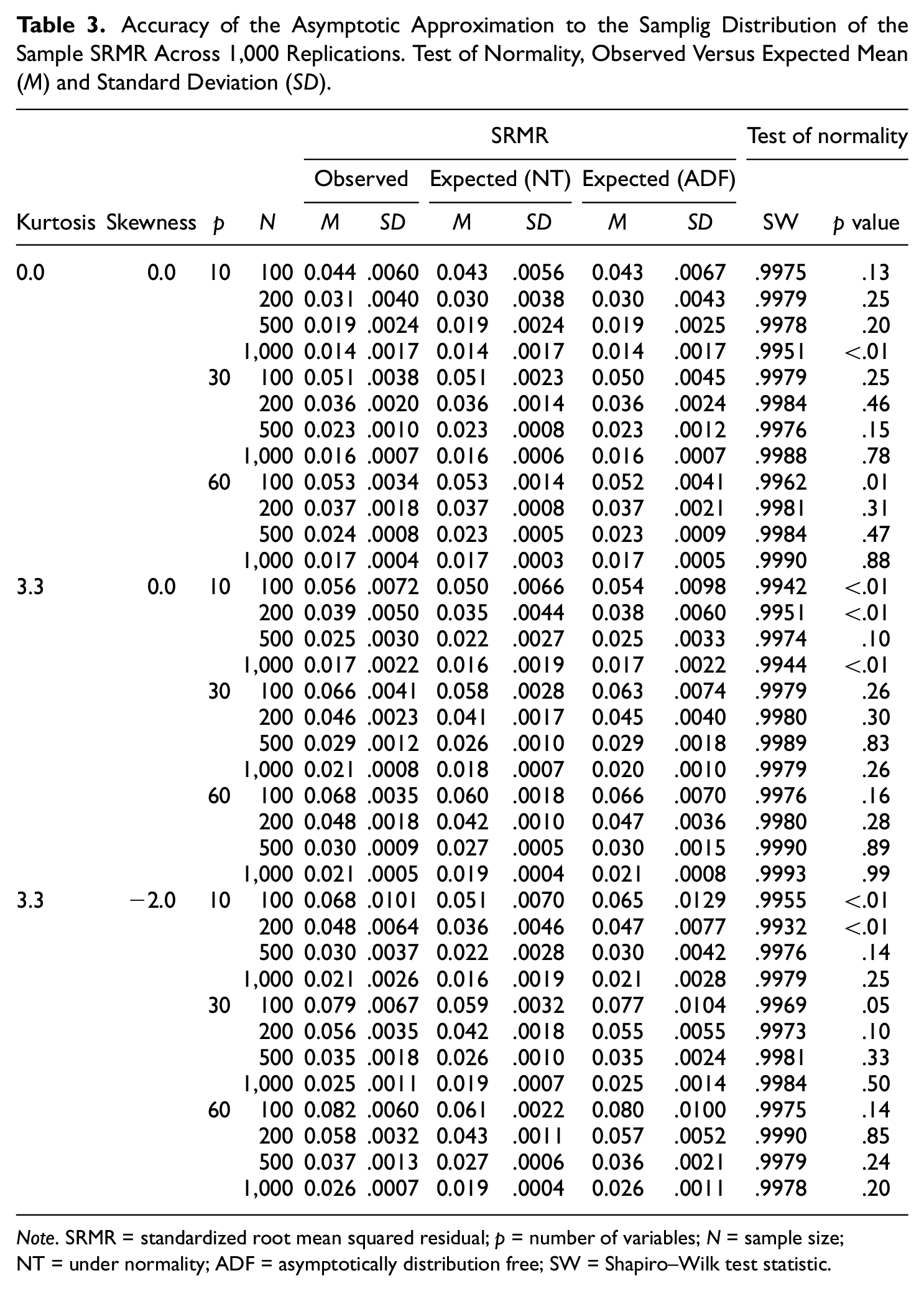
Note. SRMR = standardized root mean squared residual; p = number of variables; N = sample size; NT = under normality; ADF = asymptotically distribution free; SW = Shapiro–Wilk test statistic.
We illustrate this issue in Figure 2. In this figure, we provide histograms of the
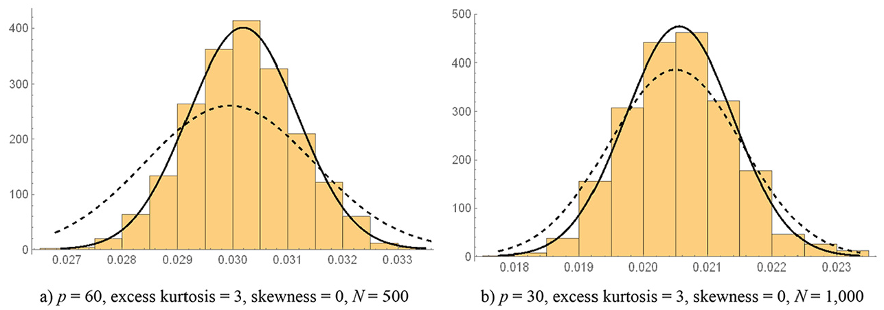
Empirical distribution of the sample standardized root mean squared residual (SRMR) and reference normal distributions. (a) p = 60, excess kurtosis = 3, skewness = 0, N = 500; (b) p = 30, excess kurtosis = 3, skewness = 0, N = 1,000.
In the other condition displayed in Figure 2, with N = 1,000, p = 30, (excess) kurtosis = 3, and skewness = 0, the relative bias of the expected mean of the
As depicted in Figure 2, distribution of the sample SRMR appears to be quite normal. To further assess the quality of the normal approximation to the distribution of the sample SRMR, we performed Shapiro and Wilk’s (1965) test of normality for each of the investigated conditions. We chose this particular test as it has been shown to be the most powerful to detect departures from normality (Yap & Sim, 2011). The test statistic ranges from 0 to 1, with 1 indicating perfect fit. In out study, the statistic ranged from .993 to .999 across conditions (see Table 3), indicating that a normal distribution provides a good fit to the sampling distribution of the SRMR. We have also provided in Table 3 p values for this test statistic because they may more clearly pinpoint conditions under which the normal approximation works best. As it may be observed in the table, the main driver of the accuracy of the normal approximation is model size. Specifically, the normal approximation is somewhat poorer when the number of observed variables is small (i.e., p = 10).
Concluding Remarks
In the current study, we investigated whether a recently proposed test statistic (based on the SRMR) outperforms the current standard tests to evaluate the exact fit of structural equation models in terms of Type I errors. We conclude that the answer is negative. Because the current standard test statistics are a side product of the computations involved in obtaining maximum likelihood parameter estimates and standard errors, the current test statistics are to be preferred to the new proposal. We have not compared the power of both approaches as it only makes sense to compare the power of test statistics when accurate Type I errors are obtained, which was not the case in many of the conditions investigated.
The accuracy of the SRMR test of exact fit depends on the accuracy of the reference nomal distribution to the sampling distribution of the SRMR, and on the accuracy of the asymptotic approximation to the empirical mean and standard deviation of the sampling distribution of the SRMR. We found that the proposed reference normal distribution provides a good approximation to the sampling distribution of the SRMR when the model fits exactly, but additional statistical theory is needed to support the use of this reference distribution. We also found that the asymptotic approximation to the mean of the SRMR sampling distribution is quite accurate, but that the asymptotic approximation to the standard deviation is not. Under normality assumptions, the asymptotic approximation underestimates the empirical standard deviation; under asymptotically distribution free assumptions, it overestimates it. The reason for the differential accuracy of the asymptotic approximations to the empirical mean and standard deviation is that two terms are used to approximate the mean, but only one term is used to approximate the standard deviation (for technical details, see Maydeu-Olivares, 2017a). The present study sugests that a two-term approximation is needed also for the standard deviation. Further statistical theory is required to obtain a better asymptotic approximation to the empirical sampling distribution of the SRMR and to support the use of a reference normal distribution.
Supplemental Material
EPM-20-0043_supplementary_materials_FINAL – Supplemental material for Using the Standardized Root Mean Squared Residual (SRMR) to Assess Exact Fit in Structural Equation Models
Supplemental material, EPM-20-0043_supplementary_materials_FINAL for Using the Standardized Root Mean Squared Residual (SRMR) to Assess Exact Fit in Structural Equation Models by Goran Pavlov, Alberto Maydeu-Olivares and Dexin Shi in Educational and Psychological Measurement
Footnotes
Declaration of Conflicting Interests
The author(s) declared no potential conflicts of interest with respect to the research, authorship, and/or publication of this article.
Funding
The author(s) disclosed receipt of the following financial support for the research, authorship, and/or publication of this article: This research was supported by the National Science Foundation under Grant No. SES-1659936.
Supplemental Material
Supplemental material for this article is available online.
Notes
References
Supplementary Material
Please find the following supplemental material available below.
For Open Access articles published under a Creative Commons License, all supplemental material carries the same license as the article it is associated with.
For non-Open Access articles published, all supplemental material carries a non-exclusive license, and permission requests for re-use of supplemental material or any part of supplemental material shall be sent directly to the copyright owner as specified in the copyright notice associated with the article.