Examining Multidimensional Measuring Instruments for Proximity to Unidimensional Structure Using Latent Variable Modeling

Abstract

A widely applicable procedure of examining proximity to unidimensionality for multicomponent measuring instruments with multidimensional structure is discussed. The method is developed within the framework of latent variable modeling and allows one to point and interval estimate an explained variance proportion-based index that may be considered a measure of proximity to unidimensional structure. The approach is readily utilized in educational, behavioral, and social research when it is of interest to evaluate whether a more general structure scale, test, or measuring instrument could be treated as being associated with an approximately unidimensional latent structure for some empirical purposes.

Keywords

bifactor model global factor index of proximity to unidimensionality latent variable modeling latent structure local factor multicomponent measuring instrument unidimensionality

Educational, behavioral, and social science research is frequently based on or utilizes multiple-component measuring instruments (e.g., tests, scales, inventories, self-reports, questionnaires, surveys, test batteries, testlets, or subscales; McDonald, 1999). Part of the reason for their high popularity in these and cognate disciplines is their widely appreciated feature of providing multiple converging pieces of information about underlying latent constructs of main interest (e.g., Raykov & Marcoulides, 2011). A major activity routinely recommended to engage in prior to using these instruments is the examination of their latent structure (e.g., Mulaik, 2009). While that of unidimensionality is frequently desirable, empirical research in these sciences oftentimes evolves within settings where primarily for validity-related reasons an instrument under consideration may not possess a (strictly) unidimensional latent structure. Under those circumstances it is important for a scholar to be in a position to evaluate the degree to which its latent structure may be close to, or alternatively far from, unidimensional, with the view of possibly employing the instrument in the former case as approximately unidimensional for some substantive purposes in its applications.

Over the past couple of decades, essential unidimensionality has received considerable interest by educational and behavioral scientists (e.g., Reise, 2012; cf. Nandakumar, 1991). Much of this research has developed within the framework of the increasingly popular bifactor model (e.g., Reise et al., 2010). This model stipulates that each of a given set of observed variables loads on a “global” factor and in addition on a “local” factor related only to an appropriate subset of variables, with the global and local factors assumed uncorrelated for identification purposes (see also Eid et al., 2017; Eid et al., 2018; for additional discussions of model identification and related issues). The bifactor model may be seen as being highly structured due to having one or more local factors, which are often deemed of a lesser subject-matter relevance than the global (overall) factor loading on all manifest measures. These complexity-related properties of the model seem to limit though its applicability to situations where its restrictive multifactorial structure is plausible for a given study and/or analyzed data set. In addition, the bifactor model reflects a particular multidimensional structure, with a single possibly dominant dimension relating to all observed variables, whereas the question of proximity to unidimensional structure is relevant in principle with any multidimensional structure. However, as advocated for in the remaining discussion, the conceptual idea underlying the bifactor model can also be utilized in empirical settings where it is of interest to address the potentially highly relevant issue of proximity to unidimensional structure for an instrument associated with a latent structure more complex than that of unidimensionality.

The present note is concerned with the question of how one could evaluate the extent to which a multicomponent measuring instrument with two or more underlying factors possesses a latent structure approximating unidimensionality. The following discussion is initially concerned with a latent variable modeling (LVM; B. O. Muthén, 2002) procedure for point and interval estimation of an index quantifying empirically and theoretically important aspects of the “distance” between a two-dimensional and a unidimensional latent structure. The extant measurement literature does not seem to have addressed this issue to a sufficient extent, and therefore, this article aims to contribute to closing that gap in relation to evaluation of the discrepancy between unidimensionality and a more general latent structure of a multicomponent instrument (observed variable set). The LVM method described below is readily and widely applicable in research with measuring instruments that owing to various validity-related reasons—for example, construct underrepresentation (e.g., Messick, 1995)—possess in particular a two-dimensional latent structure, that is, one characterized by two factors rather than a single factor. The described approach is straightforwardly extended, however, to cases with more than two underlying factors, and is illustrated using a pair of examples with empirical and simulated data.

Notation and Assumptions

This article makes extensive use of the popular confirmatory factor analysis framework (e.g., Bollen, 1989). Suppose X₁, X₂, . . ., X_k (k > 2) denote the k (approximately) continuous components of a given measuring instrument; that is, their number is finite and fixed beforehand, like these k manifest variables that are thus not sampled from a potentially infinite pool of measures (or approach such a pool). For example, the measures X₁, X₂, . . ., X_k can be the k subtests in a test battery, k testlets within an overall test, or k subscales of a psychometric scale. We advance also the frequent assumption that the instrument is utilized with (an appropriate sample from) a studied single-level, single-class population, that is, a population with no clustering effects and consisting of a single as opposed to multiple latent classes (e.g., Raykov et al., 2016; see also the “Conclusion” section).

We further posit in the remainder the validity of the common factor model for the above k components (e.g., Mulaik, 2009). That is, the following model, denoted M0, is assumed to be true (correct) for them:

\underline{X} = \underline{μ} + Λ \underline{η} + \underline{ε}

(1)

where $\underline{X}$ is the k× 1 vector of the observed measures X₁, X₂, . . ., X_k and $\underline{μ}$ is the k× 1 vector of their means. (Throughout this article, underlining is used to denote vector.) In Equation 1, Λ designates the k×q factor loading matrix (q≥1) that may but need not include cross-factor loadings and reflects the assumption that each factor loads on at least two manifest variables. In addition, $\underline{η}$ is the q× 1 vector of factors there, which are assumed with mean 0 and unit variance as well as with an unconstrained positive definite q×q covariance matrix Φ. Last but not least, in Equation 1, $\underline{ε}$ represents the k× 1 vector of unique factors (residual terms) assumed with positive variance and uncorrelated with the factors as well as among themselves.

As indicated earlier, this article will be concerned primarily with model M0 when q = 2, which for convenience we will refer to as a “two-dimensional latent structure,” but its method is directly extended to more general models with q > 2 along the lines of the following discussion (see the “Conclusion” section). A version of model M0 with k = 10, q = 2, and m = 5 observed measures per factor is depicted in Figure 1; this model will be of particular interest in the illustration section. In addition, we would argue that using robust estimation the method outlined next can be in general applied in a trustworthy way also in empirical studies involving items with at least five to seven categorical response options (e.g., Rhemtulla et al., 2012; see also Raykov & Marcoulides, 2016). Thereby, as alluded to earlier, the approach discussed below is applicable with no cross-loadings as free parameters in the matrix Λ (e.g., Figure 1), as well as alternatively with such cross-loadings, as long as the initial model M0 and model M1 defined in the following section are identified (e.g., using loading or latent variance fixing at 1 or appropriate covariance fixing at 0; this identifiability assumption, possibly after suitable parameter restrictions, is made for all models used in the article).

Figure 1.

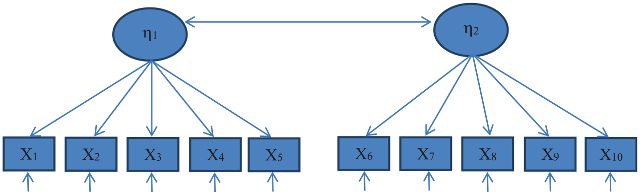
Model M0, for k = 10, q = 2, and m = 5 indicators per factor (short one-way arrows represent the unique factors that are not additionally symbolized to avoid graphical clutter).

A Latent Variable Modeling Procedure for Examining Latent Structure Proximity to Unidimensionality

Prior Research

The general issue of latent structure proximity to unidimensionality has received considerable attention in the methodological and substantive literature over the past several decades. In the context of a bifactor model for example, Raykov and Pohl (2013) discussed a proportion-explained variance-based index as a possible measure of essential unidimensionality. (As indicated earlier, a bifactor model is defined as one where each manifest measure is related to a pair of factors—a global factor that loads on all observed variables and a local factor loading only on a subset of them including the measure; for example, Reise, 2012; see also, Eid et al., 2017; Eid et al., 2018.) This index was defined as the proportion of observed overall scale variance attributable to the global factor (see Equation 2 for a formal definition), and due to some of its characteristic features it is also of relevance to the present article.

An alternative approach to essential unidimensionality was discussed in Nandakumar (1991) and based on the consequential assumption of the number of observed binary items increasing without bound (see also Stout, 1987, 1990). That earlier approach is not of concern for the aims of this article, however, since the former possesses arguably very limited applicability in contemporary empirical research. The reason is that its above asymptotic assumption with respect to number of observed components is violated in all present-day educational and behavioral studies, which in addition oftentimes utilize measures that are not binary or binary scored as assumed by that approach (see also Raykov & Marcoulides, 2018a). Furthermore, unlike that past research, this note is concerned with the setting where the number k of nonbinary measures is finite and prefixed (typically up to a few dozens at the most). As explicitly stated in the preceding section, in the current article this number of used components, k, is not increasing or approximating in any sense a set of items with an unbounded number of elements that are only of relevance for the setup underlying Nandakumar’s (1991) work (see also Stout, 1987, 1990).

Returning to the setting of concern to this note, as described before (see previous section), in order to outline the procedure of relevance in the remainder let us denote by g the global factor in a bifactor model assumed for a multicomponent measuring instrument under consideration, and by f₁, . . ., f_r (r > 0) its local factors (e.g., Figure 1 in Raykov & Pohl, 2013; cf. above Equation 1 as well as Figure 2). The earlier mentioned proportion-explained variance-based index, denoted by π_g, was defined in the last cited source as

π_{g} = \frac{λ_{1 g}^{2} + λ_{2 g}^{2} + \dots + λ_{kg}^{2}}{λ_{1 g}^{2} + λ_{2 g}^{2} + \dots + λ_{kg}^{2} + \sum_{j, s} λ_{js}^{2} + \sum_{j = 1}^{k} θ_{j}} .

(2)

Figure 2.

Model M1, for k = 10, q = 2, and m = 5 indicators of the “local” factor (short one-way arrows represent the unique factors; cf. Figure 1).

In Equation 2, λ_jg are the observed measure loadings on the global factor g, λ_js are those on the respective local factors f₁, . . ., f_r, and θ_j are the unique factor variances (residual variances) (j = 1, . . ., k, s = 1, . . ., r; we note that in general some of the loadings on a local factor may be additionally assumed vanishing; see below). That is, π_g is the proportion of observed variance, accumulated across all manifest measures, which is explained in terms of the global factor. With this property, π_g is distinct from related essential unidimensionality indices in the bifactor modeling literature that have been also considered, in that π_g is defined as a proportion of observed variance, rather than proportion of latent variance, which is explained by the global factor (cf. Reise, 2012).

Model Comparison, Testing, and Relation to Studying Proximity to Unidimensionality

In the context of proximity to unidimensional structure, we would like to make several important points before proceeding further. First, the question of proximity does not necessarily imply the need for relative model testing in most empirical settings where this query is raised. That is, whenever an applied researcher asks a question about proximity to unidimensional structure, he or she is in effect primarily interested in quantifying the “distance” between unidimensionality on one hand and the latent structure of an instrument under consideration (observed variable set) on the other hand. It is this specific question that the present article is concerned with and in this sense complements the voluminous literature on model comparison (see also next). Second, we would like to argue that the question of model testing, particularly, of a more complex model relative to that of unidimensionality, is not nearly as relevant then—if at all—owing to the fact that test statistics are affected potentially to an intolerable degree by sample size. In these cases, as is well known, the associated p-value is not sufficiently informative. For this reason, one needs alternative and complementary quantities, such as effect size measures, in order to conduct a more informed model comparison. To respond to this need, the present article is dealing with an application of what may be seen as an effect-size measure, namely, the index π_g from Equation 2 (see also the discussion in the next section), which may be very useful for the purpose of comparing the latent structure of a given measuring instrument with that of unidimensionality. Third, empirical researchers are frequently concerned with the query whether they could use an instrument (observed component set) as effectively unidimensional in a practical application. This may well be the case irrespective of whether the more complex (i.e., multidimensional) model may be fitting a given data set in some sense better than that of unidimensionality. The interest in this article lies instead with quantifying the proximity to unidimensional structure to begin with, and none of the following discussion is meant to imply that model comparison or testing should be abandoned when concerned with examining this proximity. Last, and no less important, the multidimensional models of concern in the rest of the article are not nested in each other since neither of them is obtainable from the other by merely restricting (or only adding/releasing) parameters.¹

How to Quantify Proximity to Unidimensional Structure—A Useful Proposal

The above cited research, despite being focused on the bifactor model, provides as indicated earlier a useful approach to quantification of proximity to unidimensionality. In particular, based on that prior work, we propose employing (a) the index π_g in Equation 2 and (b) the method for its point and interval estimation described in Raykov and Pohl (2013), as a means of evaluating the “proximity” of a two-dimensional latent structure to that of unidimensionality (see also the “Conclusion” section for extension to a more general multidimensional structure). In order to facilitate this use of π_g however, we observe that it has been originally defined for the bifactor model, which in general does not possess a two-dimensional latent structure that is of particular concern to this note. In fact, even if r = 1 when a corresponding bifactor model is characterized by q = 2 latent factors (1 global and 1 local factor), the latter model is not identical or equivalent to a model with a general two-dimensional latent structure, that is, model M0 with q = 2 as defined in Equation 1 (see Figures 1 and 2).

Therefore, in order to make it possible to utilize the above index π_g (Equation 2) for our purposes, we introduce a “bridging” model between model M0 and a bifactor model. The bridging model has a two-dimensional structure (i.e., it is characterized by q = 2 factors), is denoted M1 in the rest of this article, and retains many features of M0. Specifically, model M1 is defined as follows:

\underline{X} = \underline{μ} + Γ \underline{κ} + \underline{δ}

(3)

where $\underline{X}$ and $\underline{μ}$ are the same vectors as in Equation 1 and $\underline{δ}$ is the k× 1 vector of associated unique factors (assumed uncorrelated among themselves and with the latent factors; see next). In addition, in Equation 3, $\underline{κ}$ denotes the 2 × 1 vector of uncorrelated and appropriately reconceptualized factors as follows, with 0 mean and unit variance, in order to achieve the relevant parameterization for our aims of the loading matrix Γ (1 < m < k):

Γ = [\begin{matrix} γ_{11} & 0 \\ γ_{21} & 0 \\ γ_{31} & . . . \\ . . . & γ_{12} \\ γ_{k - 1, 1} & . . . \\ γ_{k 1} & γ_{m 2} \end{matrix}] .

(4)

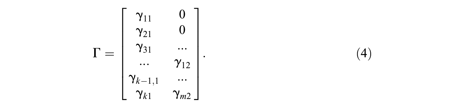
In Equation 4, all loadings on the first factor κ₁—which can be conceived of as a global factor here—are free parameters and denoted by γ_j1 (j = 1, . . ., k). Furthermore, the second factor κ₂—conceived of as a local factor—loads only on the same m observed measures that the factor η₂ in model M0 loads on. (That is, in the second column of Γ only γ₁₂, . . ., γ_m2 are free parameters.) Moreover, in model M1 all cross-loadings that are present in M0 (if any) are retained as loadings of the factor κ₂. Last, all loadings of the factor η₂ in model M0 are also loadings of the factor κ₂ in M1, while all observed measures load on the global factor κ₁. A special case of model M1, with k = 10, q = 2, and m = 5 indicators of the local factor, which corresponds along the lines of this discussion to the initial model M0, is depicted in Figure 2 (compare with Figure 1) and will be of particular interest in the illustration section, where it will be employed in an instrumental fashion in its data examples.

It is worthwhile emphasizing that model M1 is neither identical to model M0 nor equivalent to it. The sole purpose of considering M1 is to introduce a model that (a) is as close as possible to M0, and at the same time (b) accounts for the factor interrelationship in M0 by the loadings of the global factor in M1 on the observed measures that in M0 load on its second factor, η₂. At the same time, model M1 could be considered a bifactor model if in the definition of the latter it is included that some factor loadings may be (additionally) equal to 0. (We note that within their general definition, and as indicated earlier, bifactor models may differ in the extent to which they are restricted, permitting in particular further loadings to vanish; e.g., Gibbons & Hedeker, 1992; Hyland, 2015; Reise et al., 2010.) These loadings would then be those of the factor κ₂ in M1 on the manifest measures, that in M0 load on its factor η₁ (e.g., Figure 1 in Raykov & Pohl, 2013; see also Figures 1 and 2 in the present article). With this in mind, we can view M1 as the closest to M0 bifactor model, that is, a bifactor model that approximates maximally the two-factor model M0 of initial concern.

The benefit of considering model M1 lies in the fact that based on the preceding developments we can revisit the earlier mentioned proportion-explained variance-based index π_g in Equation 2, which was originally defined for bifactor models. To be more concrete, in line with the earlier discussion, π_g can now be utilized to evaluate the degree to which the global factor, κ₁, in model M1 dominates its local factor, κ₂. Granted the concern of the present note with approximation of a multidimensional latent structure by a unidimensional one, when applied to model M1 we will refer to π_g as an index of proximity to unidimensionality (IPU).

When the IPU is salient in an empirical study, that is, the global factor dominates to a substantial extent the local factor in a pertinent model M1, one may argue that with its dominance in terms of explained observed variance its global factor κ₁ makes the local factor κ₂ in effect superfluous (see also below). In those cases, for certain empirical and substantive purposes one could consider the instrument consisting of the above components $\underline{X}$ as being associated with an approximately unidimensional structure. Conversely, if the IPU index π_g is not (sufficiently) salient, an argument may be advanced that the instrument is inherently multidimensional (two-dimensional), and hence that it would not be reasonable to use it as an approximately unidimensional scale or test. In either case, the IPU point and interval estimates obtained thereby with the method in Raykov and Pohl (2013) play an important role—in addition to essential then substantive considerations—in supporting a conclusion in favor of one of these two alternative interpretations (see also the “Conclusion” section). (The respective interpretation guidelines for the point estimate and confidence interval of the index π_g that have been offered in the last cited source can be used thereby as well, as exemplified in the next section.) The empirical implications of either conclusion, its justification, and the delineation of the area of corresponding use of the instrument in subsequent research, would in general be deferred to subject-matter experts in the substantive field of its utilization.

The next section presents a couple of applications on empirical and simulated data of the described method for examining the proximity of the latent structure underlying a multicomponent measuring instrument to a unidimensional structure.

Illustration of Unidimensional Proximity Evaluation Procedure on Empirical and Simulated Data

We commence here with the consideration of an empirical example involving a study of one of the most widely used scales in behavioral and social research, the Positive and Negative Affect Schedule (PANAS; Watson et al., 1988; Watson & Tellegen, 1985). Although affect might be construed along a circumplex structure with positive and negative affect forming polar opposites (e.g., Russel, 1980; Warr, 1990), the PANAS questionnaire is known to represent a two-dimensional instrument with weakly correlated factors for positive and negative affectivity, respectively (see also, Tellegen et al., 1999, for a discussion of the dimensionality of affect). Therefore, aggregating items that reflect positive and negative affectivity in order to form an index of overall affectivity (after appropriate recoding of “inverse” items) need not be legitimate, as it could incur substantial loss of information since proximity to unidimensionality may be a far from tenable hypothesis (and in fact unidimensionality was not originally intended for the PANAS instrument; cf. Watson et al., 1988).

In this context, we analyze next the 10 (= 2 × 5) items of the international PANAS short form using publicly available data from U.S. (n = 346) respondents found at https://osf.io/a5pze (Anvari & Lakens, 2019). This scale has been developed with the aim of maximizing cross-cultural comparability, and is oftentimes referred to as the I-PANAS-SF instrument (Thompson, 2007). In the following analyses, we wish to examine the proximity of its latent structure to that of unidimensionality. In line with the preceding discussion, we first fit the single-factor model of (strict) unidimensionality (i.e., model M0 with q = 1), which is found to be associated with poor fit: chi-square value (χ²) = 330.816, degrees of freedom (df) = 35, p value (p) = .0, and root mean square error of approximation (RMSEA) = .156 with a 90% confidence interval (CI) being [.141, .172]. When fitting model M0 with two correlated factors, however (see Figure 1), the resulting overall fit indices suggest a tenable model: χ² = 43.425, df = 34, p = .129, and RMSEA = .028 (90% CI = [.000, .051]). The factor correlation estimate is thereby .045, which additionally indicates that the data are not close to supporting a (strictly) unidimensional latent structure. Fitting then model M1 with a global and a local factor (see Figure 2) yields also tenable and markedly better fit indices relative to M0: χ² = 34.764, df = 30, p = .251, RMSEA = .021 (90% CI = [.000, .048]). (The Mplus input file that can be used for this purpose is provided in Appendix A.) Table 1 contains its parameter estimates along with their standard errors, t values, and p values.²

Table 1.

Parameter Estimates in Model M1 for the Empirical Data Example (Used Software Presentation Format).

Parameter	Estimate	Standard error	t-value	p-value
F1 BY
Y1	0.488	0.056	8.708	0.000
Y2	0.587	0.059	9.973	0.000
Y3	0.712	0.059	12.017	0.000
Y4	0.619	0.058	10.614	0.000
Y5	0.668	0.062	10.760	0.000
Y6	0.114	0.070	1.616	0.106
Y7	0.004	0.055	0.079	0.937
Y8	0.039	0.058	0.662	0.508
Y9	0.060	0.057	1.054	0.292
Y10	−0.102	0.074	−1.366	0.172
F2 BY
Y6	0.755	0.074	10.248	0.000
Y7	0.343	0.069	5.000	0.000
Y8	0.696	0.066	10.467	0.000
Y9	0.546	0.067	8.184	0.000
Y10	0.775	0.074	10.446	0.000
F1 WITH
F2	0.000
Intercepts
Y1	3.127	0.050	63.060	0.000
Y2	2.841	0.054	52.980	0.000
Y3	2.835	0.058	49.197	0.000
Y4	3.405	0.052	65.919	0.000
Y5	3.075	0.059	52.417	0.000
Y6	4.104	0.059	69.600	0.000
Y7	4.445	0.049	90.713	0.000
Y8	4.283	0.053	81.306	0.000
Y9	4.393	0.051	85.704	0.000
Y10	3.705	0.063	59.265	0.000
Variances
F1	1.000
F2	1.000
Residual variances
Y1	0.613	0.056	10.896	0.000
Y2	0.650	0.065	9.998	0.000
Y3	0.642	0.065	9.933	0.000
Y4	0.540	0.062	8.710	0.000
Y5	0.745	0.080	9.292	0.000
Y6	0.619	0.083	7.505	0.000
Y7	0.713	0.072	9.896	0.000
Y8	0.475	0.061	7.835	0.000
Y9	0.607	0.069	8.757	0.000
Y10	0.741	0.102	7.270	0.000
New/additional parameters
IPU_G	0.188	0.017	10.978	0.000
IPU_L	0.200	0.018	10.949	0.000
IPU_E	0.612	0.020	30.498	0.000

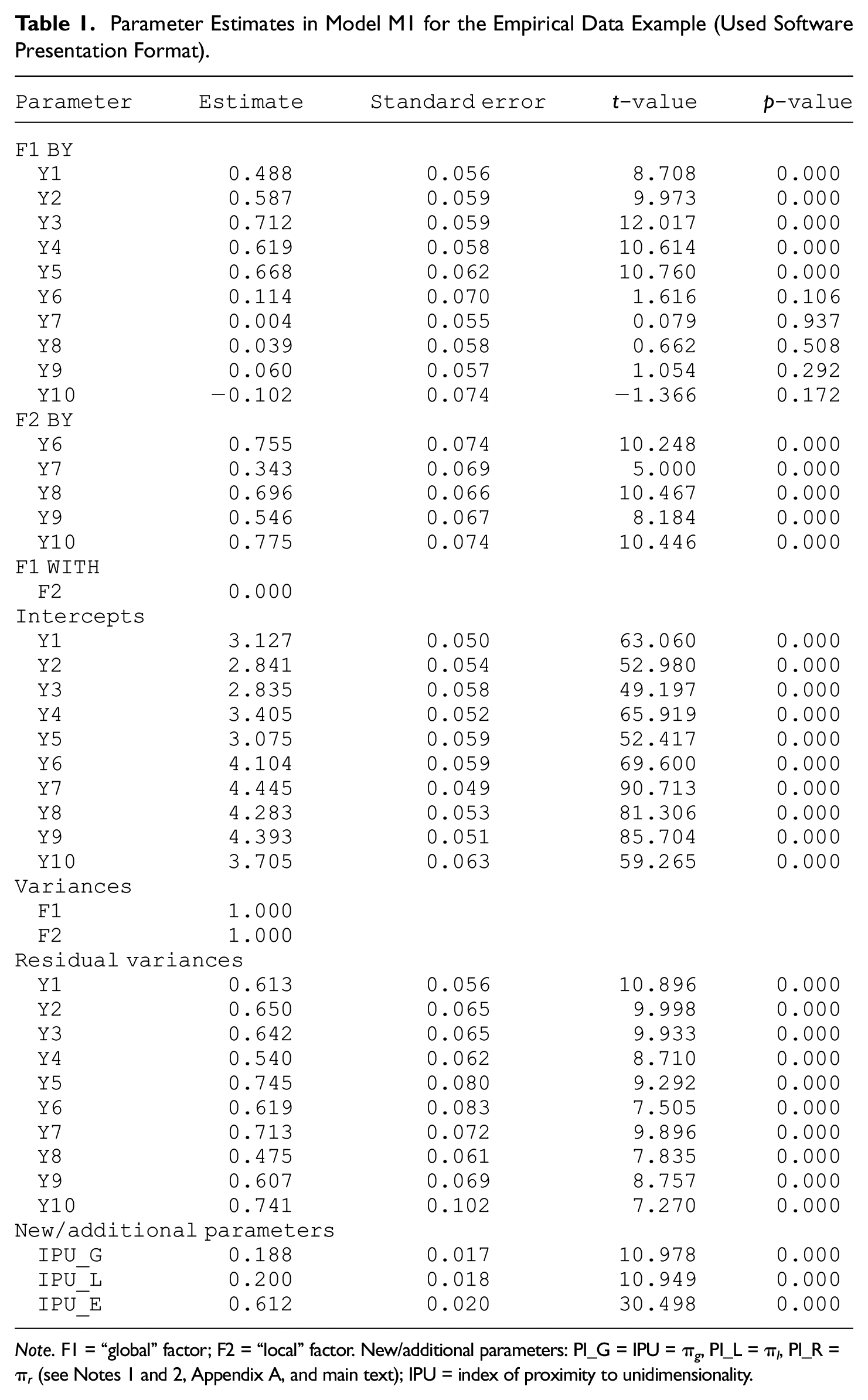
Note. F1 = “global” factor; F2 = “local” factor. New/additional parameters: PI_G = IPU = π_g, PI_L = π_l, PI_R = π_r (see Notes 1 and 2, Appendix A, and main text); IPU = index of proximity to unidimensionality.

The above results, along with the earlier discussion in this note, may suggest that an empirical scholar could be tempted to use model M1 in subsequent research with the I-PANAS-SF instrument. To examine further a possible rationale behind such a suggestion, we turn to the critical IPU estimate in this model (see Table 1), which is ${\hat{π}}_{g} =$ .188 (.017) (using a circumflex to denote estimate, with standard error following in parentheses, as in the rest of this article). Employing next the R-function “ci.ipu” provided in Appendix C we obtain the following 95% CI for the IPU = [.157, .224]. Furthermore, the estimate of the proportion of observed variance explained by the local factor is thereby ${\hat{π}}_{i} =$ .200 (.018) (95% CI = [.167, .238]).³ In addition, the proportion of observed variance due to the unique factors (residual variances) is estimated as ${\hat{π}}_{r} =$ .612 (.020) (95% CI = [.572, .650]).⁴

For the interpretation of the above IPU estimate, we use now the informal guidelines provided by Raykov and Pohl (2013). (See in particular the discussion of the 70:20:10 interpretation guides offered there—accordingly, a global factor underlying an instrument under consideration may be viewed for some empirical purposes as dominating its local factors if it explains at least 70% of the variance in the analyzed set of observed variables; the remaining variance would then be explained by the local factors and residuals; for further details, we refer to the above-cited source.) With this in mind, we observe that the CI of the IPU, $π_{g}$ , overlaps to a substantial degree with the CI of the proportion of observed variance due to the local factor, $π_{i}$ , with both of these intervals not exceeding the mid .20s and positioned entirely to the left of the CI of the residual proportion of observed variance, $π_{r}$ . These results indicate a lack of dominance of the global factor, which along with the comparable variance explanatory power of the local factor reveals a finding of a marked distance of the latent structure of the PANAS short scale under consideration from that of unidimensionality. Therefore, one may conclude that the latent structure underlying the I-PANAS-SF instrument consisting of the 10 items in question is not approximately unidimensional.

In the second example, we employ simulated data to demonstrate further the utility and applicability of the discussed unidimensionality proximity estimation procedure. The benefit of using here simulated data derives from the observation that unlike the last example where the true structure was unknown, we have now access to the model having generated the data and can thus judge the degree to which the described IPU evaluation method leads to results consistent with that model’s features. More specifically, we utilize next multinormal data generated for n = 1,000 cases on k = 10 components using the following two-factor model (see Figure 1):

\begin{matrix} X_{1} = η_{1} + ε_{1}, \\ X_{2} = 1.3 η_{1} + ε_{2}, \\ X_{3} = 1.5 η_{1} + ε_{3}, \\ X_{4} = 1.7 η_{1} + ε_{4}, \\ X_{5} = 1.3 η_{1} + ε_{5}, \\ X_{6} = . 8 η_{1} + ε_{6}, \\ X_{7} = . 3 η_{2} + ε_{7}, \\ X_{8} = . 4 η_{2} + ε_{8}, \\ X_{9} = . 5 η_{2} + ε_{9}, \\ X_{10} = . 5 η_{2} + ε_{10}, \end{matrix}

(5)

where η₁ and η₂ were standard normal random variables with correlation ρ = .55, while the error terms ε₁ through ε₁₀ were independent zero-mean normal variables with variance .3 each. (The Mplus command file used for data simulation is provided in Appendix B, including the seed employed, in order to facilitate replication of the following results; L. K. Muthén & Muthén, 2020.)

Fitting first model M0 (with k = 10, q = 2, and m = 5 indicators per factor and no cross-loadings; see Figure 1) to the so-generated data set yields, as expected, tenable overall fit indices, since this model is identical in structure to that utilized in the simulation process: χ² = 49.806, df = 34, p = .039, and RMSEA = .022 (90% CI = [.005, .034]). Like earlier, when fitting instead the model of (strict) unidimensionality—that is, the single-factor model M0 with q = 1—these fit indices are found to be clearly far from tenable: χ² = 952.900, df = 35, p = .0, RMSEA = .162 (90% CI = [.153, .171]). The results indicate that the data do not comply with a (strictly) unidimensional latent structure, a correct conclusion since the latter seriously misspecified structure did not underlie the data generation process. Yet fitting model M1 (see Figure 2) to the simulated data set is associated with tenable fit indices: χ² = 47.436, df = 30, p = .022, RMSEA = .024 (90% CI = [.009, .037]). (The Mplus command file for fitting model M1 is provided in Appendix A.) These findings suggest that model M1 (which is distinct from the model used in the data generation process) is plausible for the analyzed data set. Table 2 contains its parameter estimates along with their standard errors and associated t values as well as p values. (We note in passing that the individual measure R² indices are correspondingly nearly identical in models M0 and M1.)

Table 2.

Parameter Estimates in Model M1 for the Simulated Data Example (Used Software Presentation Format).

Parameter	Estimate	Standard error	t-value	p-value
F1 BY
X1	0.996	0.028	35.020	0.000
X2	1.315	0.034	38.590	0.000
X3	1.494	0.038	39.621	0.000
X4	1.713	0.042	40.489	0.000
X5	2.020	0.048	41.653	0.000
X6	0.434	0.030	14.620	0.000
X7	0.150	0.020	7.503	0.000
X8	0.240	0.022	10.830	0.000
X9	0.264	0.023	11.561	0.000
X10	0.254	0.024	10.684	0.000
F2 BY
X6	0.721	0.028	25.388	0.000
X7	0.237	0.021	11.155	0.000
X8	0.343	0.023	15.109	0.000
X9	0.409	0.023	17.879	0.000
X10	0.432	0.024	18.177	0.000
F1 WITH
F2	0.000
Intercepts
X1	−0.087	0.036	−2.415	0.016
X2	−0.044	0.045	−0.971	0.331
X3	−0.071	0.050	−1.415	0.157
X4	−0.099	0.057	−1.729	0.084
X5	−0.092	0.066	−1.391	0.164
X6	−0.019	0.031	−0.620	0.535
X7	0.000	0.020	−0.019	0.985
X8	0.015	0.023	0.684	0.494
X9	−0.034	0.023	−1.453	0.146
X10	−0.014	0.024	−0.566	0.571
Variances
F1	1.000
F2	1.000
Residual variances
X1	0.304	0.015	20.494	0.000
X2	0.287	0.015	18.896	0.000
X3	0.295	0.016	18.019	0.000
X4	0.311	0.018	16.902	0.000
X5	0.297	0.021	14.442	0.000
X6	0.247	0.027	9.156	0.000
X7	0.325	0.015	21.295	0.000
X8	0.334	0.017	19.992	0.000
X9	0.307	0.017	18.576	0.000
X10	0.332	0.018	18.511	0.000
New/additional parameters
PI_G	0.752	0.009	81.324	0.000
PI_L	0.064	0.004	15.350	0.000
PI_E	0.185	0.007	26.747	0.000

As seen from Table 2, the estimate of the critical IPU quantity is ${\hat{π}}_{g} =$ .752 (.009). Using again the R-function “ci.ipu” (Appendix C), we obtain the following 95% CI for the IPU = [.734, .769]. Similarly, the estimate of the proportion of observed variance explained by the local factor is ${\hat{π}}_{i} =$ .064 (.004), with a 95% CI being [.056, .072]. Furthermore, the proportion of observed variance due to the unique factors (residual variances) is ${\hat{π}}_{r} =$ .185 (.007), with a 95% CI of [.172, .199]. Employing then the above indicated, informal 70:20:10 guidelines for interpretation of the essential unidimensionality index π_g (Raykov & Pohl, 2013), which for model M1 is, as mentioned, the IPU of relevance in this article, the following may be suggested. Since (a) the CI of the IPU is entirely above .70, (b) the CI of π_l is wholly within [0, .10], and (c) the CI for π_r is completely under .20, one may suggest that the latent structure underlying the multicomponent instrument consisting of the above $\underline{X}$ measures (Equations 5) is plausibly approximated by that of unidimensionality. The specific implications of this conclusion as well as the delineation of the extent of its empirical relevance and utility, as indicated earlier, are generally deferred to subject-matter experts in the substantive field of instrument application.

Conclusion

This note addressed the query of how one could ascertain whether a multidimensional multicomponent measuring instrument may be associated with a latent structure that is approximately unidimensional. A point and interval estimation procedure based on latent variable modeling was discussed, which can be used to evaluate the “distance” between a two-dimensional latent structure of a set of observed measures (instrument components) and a unidimensional structure (see also below). An IPU aimed at quantifying this distance, in the metric of proportion-observed overall variance attributable to a suitably defined global factor, was discussed as a measure of the discrepancy between two-dimensional and unidimensional latent structures. Due to its particular definition (see Equation 2), the IPU may also be viewed as an effect size measure of the “distance” between the latent structure underlying a given multicomponent measuring instrument and the corresponding unidimensionality structure. It was argued that when the IPU is deemed sufficiently large based on substantive considerations in a subject-matter domain, the instrument may be used as essentially unidimensional for certain empirical purposes (see illustration section for some informal interpretation guidelines of possible utility then).

While the discussion in this article evolved predominantly within the framework of a two-factor model with correlated factors (model M0 with q = 2; e.g., Figure 1), its approach is applicable as mentioned also in more general settings with a larger number of underlying factors. To this end, a suitable subset of q− 1 from these factors are formally reconceptualized as “local” factors in a bridging model (M1), following relevant substantive considerations, which factors are then assumed unrelated to the remaining, “global” factor in M1. The latter factor explains in M1 all original relationships of an appropriately chosen factor in M0 with the rest of the factors there, via this global factor’s loadings on their own indicators in M1 that are unaltered relative to M0 (e.g., Figure 2). The same index of proximity to unidimensionality in Equation 2 can then be used as a measure of the degree of approximation of the original latent structure by that of unidimensionality.⁵

Several limitations of the procedure discussed in this article are worth indicating at this point. One, the note does not imply and is not meant to suggest that any measuring instrument’s latent structure can be approximated (well) by a unidimensional structure. It is for this reason that we discussed the IPU measure as applied within the bridging model M1. Two, the note does not mean to suggest that with its procedure one can identify the true model having generated a given data set in an empirical study. Three, while we argued in favor of using the IPU quantity π_g in educational, behavioral, and social research, we do not imply that there ought to be hard and fast cutoffs for it, especially with respect to how to interpret its point and interval estimates in an empirical setting. We referred thereby to the preliminary guides offered in Raykov and Pohl (2013; specifically, the 70:20:10 relation between π_g, π_r, and π_l, respectively) only as informal and tentative guidelines, rather than as such approaching a rule-of-thumb status. With this in mind, we leave to future research the examination of the degree to which they could be trustworthy as well as in particular the conditions under which they may be so. Four, we do not suggest that a conclusion in a given study that a used instrument may have approximately unidimensional structure would be valid for all purposes in its possible applications. In particular, one could imagine that for some of them, especially where it is relevant to capitalize on the discrepancy between the instrument’s actual latent structure and that of unidimensionality, it may not be meaningful to consider a test or scale under consideration as having approximately unidimensional structure, even if the associated IPU appears to be high. As always, substantive considerations are called for and of higher relevance while assessing (a) whether a particular empirical setting and research question(s) pursued warrant the consideration of a measuring instrument as effectively unidimensional when interpreting its IPU, and (b) for which analytic, modeling, or interpretation purposes this may be the case. Five, we do not imply that in any given empirical study a scholar will need to make a decision of sufficient proximity to unidimensionality, or lack thereof, for a used multicomponent instrument. Future studies with the same instrument (and population) may provide additional important information permitting then, rather than before them, drawing such a conclusion. In this context, we wish to also point out that we do not necessarily expect the described IPU evaluation procedure to allow one reaching an unambiguous decision in this respect in any single application or in a series of its applications with a particular measuring instrument. Six, we do not mean to suggest that the IPU discussed in this note is the only possible index (effect-size measure) that could be used when examining proximity to unidimensionality. In addition, as indicated earlier we have only considered the IPU as one possible complementary measure to model comparison that a researcher may as well be interested in during such an examination. Seven, we presumed throughout the article that the standard confirmatory factor analysis model M0 (Equation 1) is correct, or at least plausible in a given empirical study, which is basic for the entire preceding discussion. This implies that all prior work on exploring and confirming the latent structure of a multicomponent measuring instrument in question has been already conducted before considering an application of the procedure of this note, including exploratory and confirmatory analyses (factor analyses) if need be, which are recommended to be carried out on an independent sample(s) from the same studied population (e.g., Mulaik, 2009).

Moreover, we assumed the instrument components to be (approximately) continuous, and so the discussed IPU need not be meaningfully applicable when they are binary, binary scored, or highly discrete (e.g., with say three or four possible response options). As alluded to earlier, one may conjecture that the robust maximum likelihood (ML) method (e.g., L. K. Muthén & Muthén, 2020) may be used with components possessing at least five to seven possible categorical values, as in the empirical example of the previous section, unless some items possess excessive skewness like in cases with preponderance of floor or ceiling values (cf. Rhemtulla et al., 2012). Whereas the normality assumption is made when utilizing the discussed procedure with ML as in the second example of the illustration section, we point out that its use with an application of weighted least squares with large samples is possible under nonnormality of the (approximately continuous) components. In addition, we would submit that up to mild violations of normality may be handled then also by the robust ML method. With highly discrete items, an extension of the discussed IPU evaluation procedure or the development of a corresponding analogue may well be possible along the lines of Raykov and Marcoulides (2018b), which is beyond the confines of this article. Furthermore, as explicitly indicated earlier we assumed a single-class studied population. Therefore, we would like to raise caution that the proposed method—like all conventional, single-class statistical and measurement approaches—may be misleading when applied to samples from populations with substantial unobserved heterogeneity if the latter is not accounted for (cf. Raykov et al., 2016; Raykov et al., 2019). Relatedly, we presumed also no clustering effects in a studied population, but it may be suggested that minor such effects may be accommodated by the robust ML method especially with normality or under up to limited violations of it. Last but not the least, being based on ML or its robust version, or alternatively on the weighted least squares estimation method, the procedure of concern in this note is asymptotic (with respect to units of analysis rather than components), and thus, best applied with large samples. We encourage future research into possible guidelines as to when samples may be considered sufficiently large (and under which circumstances) in order for the underlying large sample theory to be viewed as having obtained practical relevance.

In conclusion, this article offers to educational, behavioral, and social scientists a readily and widely applicable procedure for evaluation of the degree to which the multidimensional latent structure of a studied multicomponent measuring instrument may be considered (well) approximated by a unidimensional structure for certain empirical purposes.

Footnotes

Appendix A

Appendix B

Appendix C

Acknowledgements

We are indebted to G. A. Marcoulides for helpful discussions on essential unidimensionality as well as instructive and critical comments on a prior version of the paper that have led to its substantial improvement. We are grateful to the editor and two anonymous referees for critical comments on an earlier version of the article. Thanks are also due to K. Bartz for valuable comments on evaluating measuring instrument dimensionality.

Authors’ Note

This research was in part carried out while T. Raykov was visiting GESIS—Leibniz Institute for the Social Sciences in Mannheim, Germany.

Declaration of Conflicting Interests

The authors declared no potential conflicts of interest with respect to the research, authorship, and/or publication of this article.

Funding

The authors received no financial support for the research, authorship, and/or publication of this article.

ORCID iD

Matthias Bluemke

Notes

References

Anvari

Lakens

(2019, November 13). SESOI—PANAS [Data files]. http://osf.io/89pcf

Bollen

K. A.

(1989). Structural equations with latent variables. Wiley.

Eid

Geiser

Koch

Heene

(2017). Anomalous results in G-factor models: Explanations and alternatives. Psychological Methods, 22(3), 541-562. https://doi.org/10.1037/met0000083

Eid

Krumm

Koch

Schulze

(2018). Bifactor models for predicting criteria by general and specific factors: Problems of nonidentifiability and alternative solutions. Journal of Intelligence, 6(3), Article 42. https://doi.org/10.3390/jintelligence6030042

Gibbons

R. D.

Hedeker

(1992). Full-information item bifactor analysis. Psychometrika, 57(3), 423-436. https://doi.org/10.1007/BF02295430

Hyland

(2015). Application of bifactor models in criminal psychology research: A guide to researchers. Journal of Criminal Psychology, 5(2), 65-74. https://doi.org/10.1108/JCP-03-2015-0011

McDonald

R. P.

(1999). Test theory. A unified treatment. Lawrence Erlbaum.

Messick

(1995). Validity of psychological assessment: Validation of inferences from persons’ responses and performances as scientific inquiry into score meaning. American Psychologist, 50(9), 741-749. https://doi.org/10.1037/0003-066X.50.9.741

Mulaik

S. A.

(2009). Foundations of factor analysis. Taylor & Francis. https://doi.org/10.1201/b15851

10.

Muthén

B. O.

(2002). Beyond SEM: General latent variable modeling. Behaviormetrika, 29(1), 87-117. https://doi.org/10.2333/bhmk.29.81

11.

Muthén

L. K.

Muthén

B. O.

(2020). Mplus user’s guide. Muthén & Muthén.

12.

Nandakumar

(1991). Traditional dimensionality versus essential dimensionality. Journal of Educational Measurement, 28(2), 99-117. https://doi.org/10.1111/j.1745-3984.1991.tb00347.x

13.

Raykov

Marcoulides

G. A.

(2011). Introduction to psychometric theory. Taylor & Francis. https://doi.org/10.4324/9780203841624

14.

Raykov

Marcoulides

G. A.

(2016). Scale reliability evaluation under multiple assumption violations. Structural Equation Modeling, 23(2), 302-313. https://doi.org/10.1080/10705511.2014.938597

15.

Raykov

Marcoulides

G. A.

(2018a). A course in item response theory and modeling with Stata. Stata Press.

16.

Raykov

Marcoulides

G. A.

(2018b). On studying common factor dominance and approximate unidimensionality in multi-component measuring instruments with discrete items. Educational and Psychological Measurement, 78(3), 504-516. https://doi.org/10.1177/0013164416678650

17.

Raykov

Marcoulides

G. A.

Chang

(2016). Studying population heterogeneity in finite mixture settings using latent variable modeling. Structural Equation Modeling, 23(5), 726-730. https://doi.org/10.1080/10705511.2015.1103193

18.

Raykov

Marcoulides

G. A.

Menold

Harrison

(2019). Revisiting the bifactor model: Can mixture modeling help assess its applicability? Structural Equation Modeling, 26(1), 110-118. https://doi.org/10.1080/10705511.2018.1436441

19.

Raykov

Pohl

(2013). On studying common factor variance in multiple component measuring instruments. Educational and Psychological Measurement, 73(2), 191-209. https://doi.org/10.1177/0013164412458673

20.

Reise

S. P.

(2012). The rediscovery of bifactor measurement models. Multivariate Behavioral Research, 47(5), 667-696. https://doi.org/10.1080/00273171.2012.715555

21.

Reise

S. P.

Moore

T. M.

Haviland

M. G.

(2010). Bifactor models and rotations: Exploring the extent to which multidimensional data yield univocal scale scores. Journal of Personality Assessment, 92(6), 544-549. https://doi.org/10.1080/00223891.2010.496477

22.

Rhemtulla

Brosseau-Liard

P. E.

Savalei

(2012). When can categorical variables be treated as continuous? A comparison of robust continuous and categorical SEM estimation methods under suboptimal conditions. Psychological Methods, 17(3), 354-373. https://doi.org/10.1037/a0029315

23.

Russell

J. A.

(1980). A circumplex model of affect. Journal of Personality and Social Psychology, 39(6), 1161-1178. https://doi.org/10.1037/h0077714

24.

Stout

W. F.

(1987). A nonparametric approach for assessing latent trait unidimensionality. Psychometrika, 52(4), 589-617. https://doi.org/10.1007/BF02294821

25.

Stout

W. F.

(1990). A new item response theory modeling approach with applications to unidimensionality assessment and ability estimation. Psychometrika, 55(2), 293-325. https://doi.org/10.1007/BF02295289

26.

Tellegen

Watson

Clark

L. A.

(1999). On the dimensional and hierarchical structure of affect. Psychological Science, 10(4), 297-303. https://doi.org/10.1111/1467-9280.00157

27.

Thompson

E. R.

(2007). Development and validation of an internationally reliable short-form of the Positive and Negative Affect Schedule (PANAS). Journal of Cross-Cultural Psychology, 38(2), 227-242. https://doi.org/10.1177/0022022106297301

28.

Warr

P. B.

(1990). The measurement of well-being and other aspects of mental health. Journal of Occupational Psychology, 63(3), 193-210. https://doi.org/10.1111/j.2044-8325.1990.tb00521.x

29.

Watson

Clark

L. A.

Tellegen

(1988). Development and validation of brief measures of positive and negative affect: The PANAS scales. Journal of Personality and Social Psychology, 54(6), 1063-1070. https://doi.org/10.1037/0022-3514.54.6.1063

30.

Watson

Tellegen

(1985). Toward a consensual structure of mood. Psychological Bulletin, 98(2), 219-235. https://doi.org/10.1037/0033-2909.98.2.219