




Abstract
This study investigated the extent to which class-specific parameter estimates are biased by the within-class normality assumption in nonnormal growth mixture modeling (GMM). Monte Carlo simulations for nonnormal GMM were conducted to analyze and compare two strategies for obtaining unbiased parameter estimates: relaxing the within-class normality assumption and using data transformation on repeated measures. Based on unconditional GMM with two latent trajectories, data were generated under different sample sizes (300, 800, and 1500), skewness (0.7, 1.2, and 1.6) and kurtosis (2 and 4) of outcomes, numbers of time points (4 and 8), and class proportions (0.5:0.5 and 0.25:0.75). Of the four distributions, it was found that skew-t GMM had the highest accuracy in terms of parameter estimation. In GMM based on data transformations, the adjusted logarithmic method was more effective in obtaining unbiased parameter estimates than the use of van der Waerden quantile normal scores. Even though adjusted logarithmic transformation in nonnormal GMM reduced computation time, skew-t GMM produced much more accurate estimation and was more robust over a range of simulation conditions. This study is significant in that it considers different levels of kurtosis and class proportions, which has not been investigated in depth in previous studies. The present study is also meaningful in that investigated the applicability of data transformation to nonnormal GMM.
Keywords
Introduction
Growth mixture modeling (GMM) is a form of finite mixture modeling that combines conventional random effects modeling with latent trajectory classes (Muthén & Asparouhov, 2015). GMM has been commonly used to detect whether qualitatively different subgroups of developmental paths exist within a population (Bauer & Curran, 2003; Muthén, 2004). In addition to this, it has more flexibility in modeling longitudinal data compared with traditional methods (e.g., hierarchical linear modeling and repeated measures analysis of variance), so GMM has been frequently employed in social science over the past two decades (Guerra-Peña & Steinley, 2016).
GMM accommodates unobserved heterogeneity in growth trajectories by employing latent classes derived from growth factors (e.g., intercept and slope) in a latent growth curve model. By including latent classes, this methodology fully captures both within-class variation (i.e., interindividual variation in each latent class) and between-class variation (i.e., variation between latent subgroups; Jung & Wickrama, 2008). Allowance of such variation in a model generally rests on the assumption of a normal distribution. This means GMM assumes that variables within each latent class are normally distributed (i.e., within-class normality; Feldman et al., 2009; Muthén & Asparouhov, 2015). In other words, the estimation of a model and its identification in GMM depend on the assumption of a mix of normal distributions, which allows for the existence of subpopulations captured by latent trajectory classes (Bauer & Curran, 2003; Wickrama et al., 2016).
Since nonnormal distributions with various degrees of skewness and kurtosis are readily found in real data, the within-class normality assumption of GMM is often considered a limiting feature (Son et al., 2019). Because of this normality assumption, GMM tends to prefer models that include spurious classes to explain the observed variable distributions to a true model, particularly when the outcomes strongly follow nonnormal distributions (Bauer & Curran, 2004; Muthén & Asparouhov, 2015). These spurious classes, which are excessively extracted, should not be understood directly as subgroups of a population with distinct developmental patterns. Although each class-specific parameter can be computed according to the result of latent class estimation, they are likely to be artificial and nonmeaningful (Brandt & Klein, 2015). However, in general cases GMM is frequently somewhat misused despite of high possibility of spurious subgroups being overextracted in a particular model design. That is because it has been taken for granted to ignore nonnormality, even though nonnormal situations frequently occur in mixture modeling analysis (McLachlan & Peel, 2000). This is why there has been little simulation research on nonnormal GMM.
To deal with nonnormality, recent articles have investigated the use of skew-t distributions for structural equation models (SEMs) and mixture models (e.g., Asparouhov & Muthén, 2016; Frühwirth-Schnatter & Pyne, 2010; Lee & McLachlan, 2014; Lin et al., 2007). GMM with distributions generated from multiple levels of nonnormality have also been examined in previous simulation studies (e.g., Bauer & Curran, 2003; Guerra-Peña & Steinley, 2016; Jung & Wickrama, 2008; Muthén & Asparouhov, 2015; Son et al., 2019). However, most of this research has been based around the performance of fit indices, such as the Akaike information criterion (AIC; Akaike, 1974), the Bayesian information criterion (BIC; Schwartz, 1978), and sample-size adjusted BIC (SBIC; Sclove, 1987), and likelihood ratio tests, such as the Lo–Mendell–Rubin adjusted likelihood ratio test (LMR-LRT; Lo et al., 2001) and the bootstrap likelihood ratio test (BLRT; McLachlan & Peel, 2000), in terms of how to determine the number of latent classes. Only several studies (Depaoli et al., 2019; Muthén & Asparouhov, 2015; Son et al., 2019) have focused on the extent to which class-specific parameter estimates are biased by the within-class normality assumption in GMM.
Furthermore, Muthén and Asparouhov (2015) investigated the degree of parameter bias according to nonnormality under only one true model with limited conditions, meaning it is somewhat difficult to generalize their results to real situations. Depaoli et al. (2019) developed Muthén and Asparouhov’s (2015) study with different settings of simulation design by examining a variety of model fit and assessment measures, extending the type of modeling misspecification and exposing estimation difficulties of skew-t GMM. But this study left several points to be developed when it comes to including various skewness or kurtosis levels of nonnormal distributions and investigating t distribution, which also belongs to skew-t family of continuous distributions. Son et al. (2019) attempted to extend their model by considering more diverse conditions for skewness as well as four types of skew-t family distribution (i.e., the normal, t, skew-normal, and skew-t), but it remained limited in terms of kurtosis levels and class proportion within the population. They took into account only one level of kurtosis and class proportion (i.e., a balanced proportion between two latent classes), meaning that the model could not be used to further understanding of the efficiency of skew-t distributions in GMM under various nonnormal conditions that may reflect empirical cases where researchers can frequently come across in real data. Thus, it remains necessary to conduct simulations that extend previous studies by exploring more practical conditions that cover various types of nonnormality.
In social science, data transformation has traditionally been used to ensure that nonnormal variables follow a normal distribution. Recently, questions have been raised about whether data normalization approaches (e.g., logarithmic transformation, Box–Cox transformation, etc.) can be applied to SEMs and mixture models (Bauer & Curran, 2003; Kline, 2016; Yuan et al., 2000).
For example, Morgan et al. (2016) tested the robustness of normalizing transformation (i.e., van der Waerden quantile normal scores in their study) against the nonnormality of outcome variables (i.e., indicators) in terms of deciding how many latent classes exist within a population under latent profile analysis (LPA). According to their results, using that method made an accuracy of class enumeration get increased. However, this simulation study was not enough regarding that only one type of transformation was adopted. Additionally, applicability of this normalizing method to nonnormal GMMs was not examined yet.
Logarithm transformation has also been employed in other applied research (e.g., Boers et al., 2010; Stanley et al., 2017), in which the target variables are normalized for smooth estimation using the designed models. Kupek (2005) examined suitability of log-linear transformation to binary variables in SEM. In that study, SEM with the sum of squares and cross-products matrix obtained by the log-linear model correctly identified the structural relation between the variables.
In contrast, there has been a lack of simulation research examining the effectiveness and meaningfulness of data transformation in GMM. Furthermore, the two main strategies (i.e., according to whether the strategy modifies raw data, they are divided into those that employ a skew-t distribution and those that are based on normalized variables) for nonnormal GMM have not yet been compared to determine which produces better performance for a variety of nonnormal distributions deriving from different levels of skewness and kurtosis.
Therefore, in the present study, simulations were conducted to compare GMM performance with different types of distribution (i.e., normal, t, skew-normal, and skew-t distribution) under a diverse range of nonnormality in the outcome variables. Additionally, the extent to which two data transformation methods (van der Waerden quantile normal scores and adjusted logarithm transformation) assert efficient performance in nonnormal GMM is also investigated. A comparison of two previous strategies (relaxing the within-class normality assumption and using data transformation on repeated measures) is then conducted to determine which of these improves the accuracy of parameter estimation for the various nonnormal conditions.
Multivariate Nonnormal Distributions
Nonnormal mixture models can fit nonnormal data considerably better than normal mixture models (Wickrama et al., 2016). To generate more parsimonious solutions, nonnormal models look to reduce the risk of the excessive extraction of latent classes due to the nonnormality. Three different distributions can be specified based on this approach: t, skew-normal, and skew-t. The t distribution is a heavy-tailed distribution with excessive kurtosis (McLachlan & Peel, 2000) and a skew-normal distribution covers strongly skewed distribution of observations (Azzalini & Valle, 1996), while a skew-t distribution accounts for both high levels of skewness and kurtosis (Lee & McLachlan, 2014). Since the normal, t, skew-normal, and skew-t are the skew-t family of continuous distributions, skew-t distributions are considered the most general form (Asparouhov & Muthén, 2016).
Unlike the fitting of a normal distribution, which shows the results of the mean and the variance-covariance of the parameters, fitting the data to a skew-t distribution produces additional information on skewness and kurtosis (Asparouhov & Muthén, 2016; Son et al., 2019). Modeling a skew-t distribution is more complicated than simply matching skewness and kurtosis because the skew parameters are important components of the variance–covariance matrix (Muthén & Asparouhov, 2015).
Considering model’s complexity caused by including additional information such as skewness and kurtosis, this study focused on the linear GMM, which is less complex than quadratic or cubic GMM. So, in this study, the intercept and slope are included in the latent growth factors of linear GMM. In latent class

where

in which
GMM generally assumes that both

where

and marginally

where the vector mixture probabilities
To apply a skew-t distribution using the process above, it is important to note that the skew parameters of
Data Transformation for Normalization
Data transformation is a conventional approach to the normalization of data (Kline, 2016; Svolba, 2006) that has been employed in a significant volume of statistical research. As such, data transformation has been recently discussed in terms of its suitability for SEMs and mixture models (Bauer & Curran, 2003; Kline, 2016; Yuan et al., 2000) in dealing with nonnormality in models (e.g., logarithmic transformation, Box-Cox transformation, etc.). This study focuses on two types of transformation that have been applied in other simulation research: van der Waerden quantile normal scores, which were tested in LPA by Morgan et al. (2016), and logarithmic normalization, which has been employed in other applied research (e.g., Boers et al., 2010; Stanley et al., 2017).
Van der Waerden quantile normal scores were proposed by van der Waerden (1952) to normalize indicator distributions. All values in the original joint-distributions are transformed into normal scores

where
Logarithmic transformation, with which data can be made to approximately conform to normality, has been the most widely used approach in practice. However, conventional logarithmic transformation can only be applied to positive values (Feng et al., 2013). To cover zero or negative values in data (e.g., temperature, eyesight test scores, and bank statements), adjusted logarithmic transformation is a useful alternative. The manipulated
Simulation Studies
Data Generation
In this article, two Monte Carlo simulation studies were conducted. An unconditional baseline GMM is generated first with two latent trajectories by using Mplus 7.4 (Muthén & Muthén, 1998-2017). The reason why only two latent subgroups are employed is that mixture models are known to exhibit poor likelihood functions, such as those that lead to a local solution or nonconvergence (McLachlan & Peel, 2000), which may generate incorrect estimations (Son et al., 2019). The residual variance for the observations is 0.5 at all time points. The means of the intercept and slope are (4, 1) for Class 1 and (0, 0) for Class 2. The variance of the intercept and slope is 1 and 0.7, respectively, meaning individual variability in the latent growth factors is allowed. In addition, the covariance between the intercept and slope is set to 0 for both Class 1 and Class 2.
As illustrated in Figure 1, Study 1 is designed to assess the performance of each distribution used in GMM. Therefore, individual GMMs with nonnormal variables are tested under various distributions, with the nonnormality untransformed. The base model used in Study 2 is the same as that in Study 1, except for the type of distribution and data transformation. In contrast to Study 1, a normal distribution is applied in Study 2 as in conventional GMM. Instead, the outcome variables are normalized by certain methodologies of data transformation.
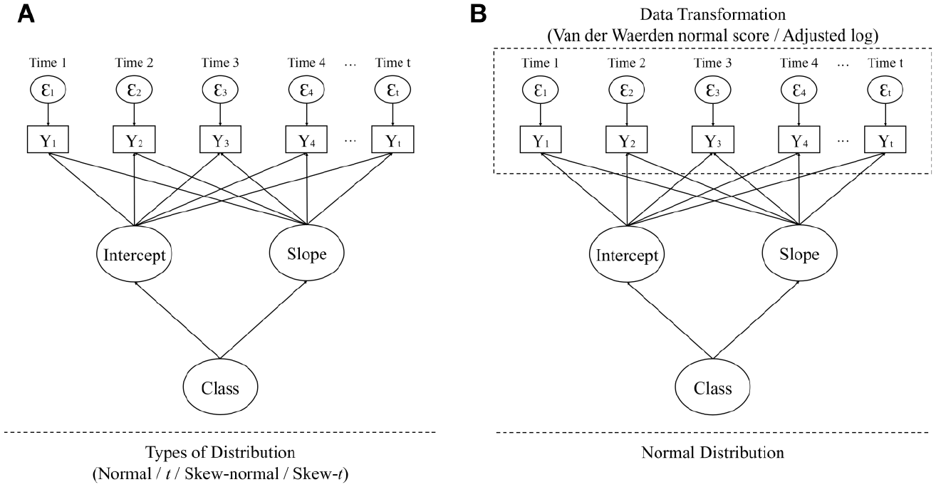
Population growth mixture modeling. (a) Study 1. (b) Study 2.
Design Factors for Simulation
Five conditions are manipulated in both Study 1 and Study 2: sample size (SS), the skewness of the outcome variables (SK), the kurtosis of the outcome variables (KT), the number of time points (NT), and the class proportion of each latent trajectory (CP). To determine the values of these conditions, previous simulation research was consulted.
Three sample sizes (300, 800, and 1,500) are considered in this study, covering the range of sample sizes frequently observed in related mixture model research (e.g., Brandt & Klein, 2015; Morgan et al., 2016; Son et al., 2019). The levels of skewness and kurtosis are manipulated as (0.7, 1.2, and 1.6) and (2 and 4) respectively. In previous simulation studies dealing with nonnormality, the skewness of the observed variables ranged from 0 to 2.28 (e.g., 0 to 1.5 in Bauer & Curran, 2003; 0 to 1.25 in Flora & Curran, 2004; 0 to 1.6 in Guerra-Peña & Steinley, 2016; 2.19 to 2.28 in Lu & Huang, 2014; 0 to 1.25 in Morgan et al., 2016), and the kurtosis ranged from 0 to 6 (e.g., 0 to 6 in Bauer & Curran, 2003; 0 to 4 in Guerra-Peña & Steinley, 2016; 0 to 3.75 in Flora & Curran, 2004; 0 to 3.75 in Morgan et al., 2016). Considering the overall conditions of nonnormality under the SEMs or mixture models, skewness and kurtosis are configured. The number of time points is set at (4 and 8) in accordance with Son et al. (2019). For the class proportion of each latent trajectory, two conditions (0.5:0.5 and 0.25:0.75) are employed based on Bauer’s (2007) simulation.
A summary of the simulation process and the design factors is presented in Table 1. A total of 72 conditions (3×3×2×2×2) are configured for data generation with 100 replications for each condition. In Study 1, the fitting of the model to each of the four distributions is conducted for the 72 conditions, while the two forms of data transformation are tested for the same 72 conditions in Study 2.
Manipulated Design Factors for the Simulations.

Note. All conditions are tested with 100 replications. CP represents the ratio of each latent class (Class 1: Class 2).
Data Transformation for Nonnormality
To generate nonnormality in the distributions of outcomes, Fleishman’s cubic transformation (Fleishman, 1978; Morgan et al., 2016; Vale & Maurelli, 1983) is applied to the data sets. This form of cubic transformation is used to obtain a specific nonnormal distribution with a certain level of skewness and kurtosis and is defined by the following polynomial expression:

where
These coefficients can be calculated using SAS/IML software (Fan et al., 2002), so SAS 9.4 is employed to generate the nonnormal GMMs in the present study. The obtained values, which derive from the skewness and kurtosis values set in the simulation design, are presented in Table 2.
Fleishman’s Transformation Cubic Coefficients.
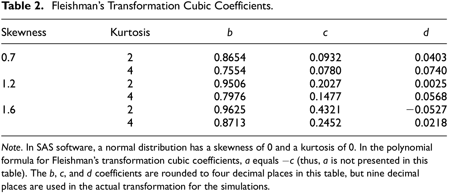
Note. In SAS software, a normal distribution has a skewness of 0 and a kurtosis of 0. In the polynomial formula for Fleishman’s transformation cubic coefficients,
Evaluation Criteria
In order to evaluate and compare the accuracy and reliability of the individual GMMs, four criteria are examined in this study: the convergence rate, parameter bias, mean square error (MSE), and coverage. The convergence rate is the number of replications in which the estimation of the analysis model is computed successfully. Therefore, nonconvergence represents that solution for the defined model may not be produced or mathematically implausible as a result of problems such as negative variance or a singular matrix. The parameter bias used in the present study is the bias of the logit for the probability of belonging to Class 1. The relative bias of this parameter can be computed using the following equation (Bandalos, 2006; Muthén & Muthén, 2000):

where

where
Results
Study 1
Study 1 investigates how the bias of the parameter estimates (i.e., the logit for probability of belonging to Class 1) is affected by the levels of nonnormality in the repeated measures using four types of distribution: normal, t, skew-normal, and skew-t. That means which distribution leads to get more accurate parameter estimates is explored. The GMMs are evaluated based on four criteria: convergence rate, parameter bias, MSE, and coverage.
Convergence Rate
The convergence rates for Study 1 according to sample size are presented in Table 3. For all conditions, GMMs with normal and t distributions exhibit good convergence rates, with all replications used in the estimation process except for a few cases. Skew-normal GMMs have the lowest convergence rates under many of the conditions, with convergence especially low for a sample size of 300, though this improved as the sample size increased. Additionally, on average, skew-normal GMMs with a CP of 0.25:0.75 have lower convergence rates compared with a CP of 0.5:0.5. Skew-t GMMs show slightly better convergence rates than skew-normal GMMs, but they remain lower than those of GMMs with normal and t distributions. In general, regardless of the distribution type, the GMMs exhibit higher convergence when the sample size is larger, the class proportion of each latent trajectory is balanced, and the degree of nonnormality is lower.
Convergence Rates in Study 1.

Note. Normally distributed condition (skewness and kurtosis of 0) is also included for convenience. SS = sample size; CP = class proportion of each latent trajectory; NT = the number of time points; SK = skewness of the outcomes; KT = kurtosis of the outcomes.
Parameter Bias
According to Table 4, the normal GMMs generate seriously biased parameter estimates. It is only under certain nonnormal conditions (SK = 1.6 and KT = 2) that the bias ranges from −0.10 to 0.10, which represents a tolerable degree of bias (Finch et al., 1997; Kaplan, 1988). Similarly, the performance of the t GMMs in terms of obtaining unbiased parameter estimates is poor, with somewhat accurate estimates produced only when NT = 4 and KT =2. On the other hand, the skew-normal GMMs produce unbiased estimates over a wider range of conditions, with an optimal performance at a sample size of 800. Unlike the GMMs with normal or t distributions, skewness affects the degree of bias to a greater extent than kurtosis for these models. Overall, however, the skew-t GMMs obtain the most accurate parameter estimates, which is consistent with past simulation research (e.g., Muthén & Asparouhov, 2015; Son et al., 2019). For most conditions, the absolute bias for this distribution is less than 0.1, but skew-t GMMs may be partially affected by kurtosis because most of the cases where the absolute bias is greater than 0.1 have KT = 4 in common.
Bias of the Logit for the Probability of Belonging to Class 1 in Study 1.
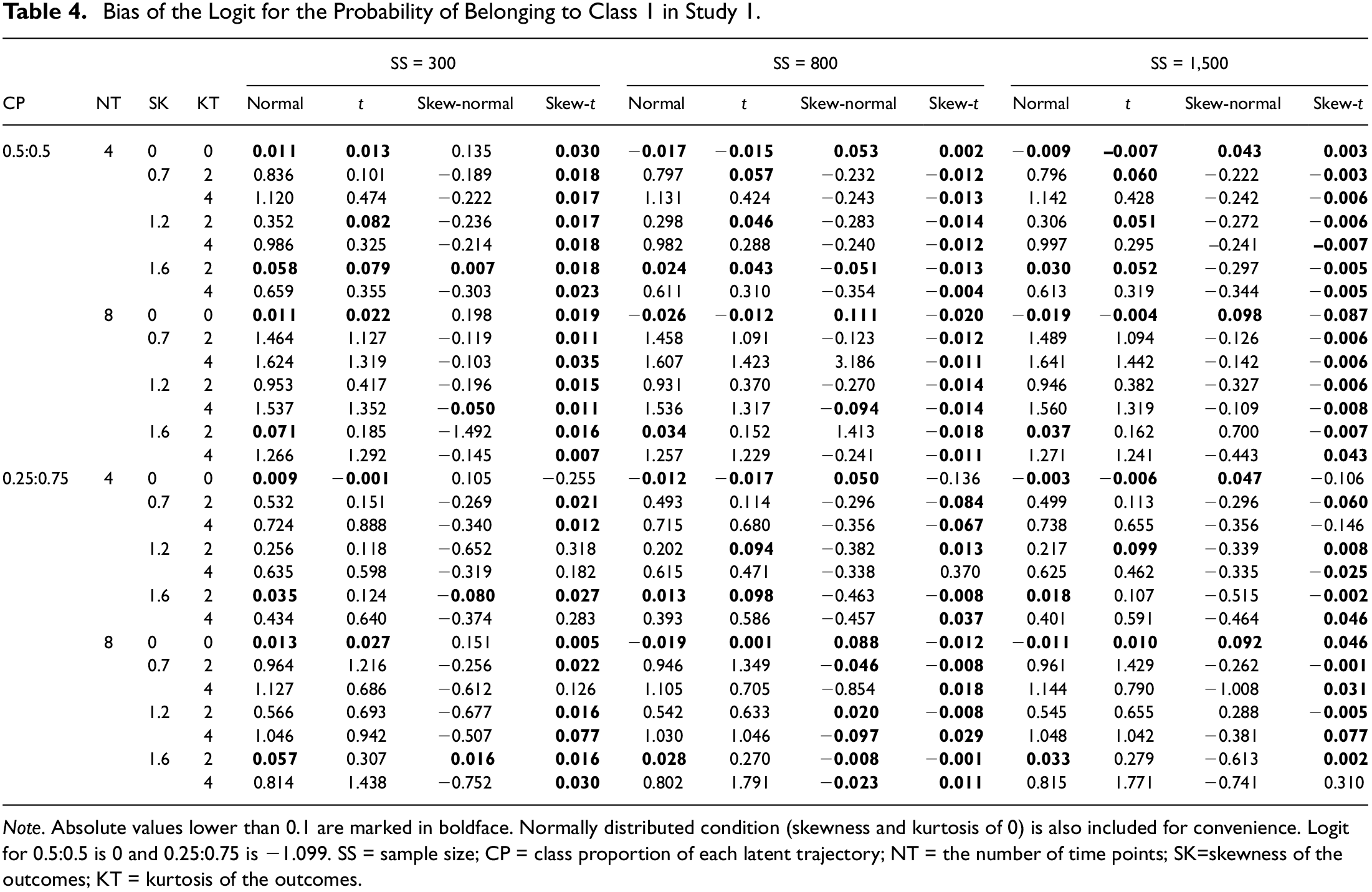
Note. Absolute values lower than 0.1 are marked in boldface. Normally distributed condition (skewness and kurtosis of 0) is also included for convenience. Logit for 0.5:0.5 is 0 and 0.25:0.75 is −1.099. SS = sample size; CP = class proportion of each latent trajectory; NT = the number of time points; SK=skewness of the outcomes; KT = kurtosis of the outcomes.
Mean Square Error
In the normal GMMs, sample size appears to have no distinguishable effect on the MSE but is affected by the other remaining factors (Table 5). On average, the t GMMs have an MSE that minutely decreases as the sample size increases. The skewness of the outcome distribution does not have a major effect on the MSE of t GMMs, but higher levels of kurtosis lead to higher MSE of t GMMs for the parameter estimates except conditions where CP = 0.25:0.75, NT = 8, and SK = 0.7. In general, the MSE is low for skew-normal GMMs. Apart from a few cases, the MSE of skew-normal GMMs is lower when the class proportion is equal for each latent class. The MSE is lowest for skew-t GMMs. A higher sample size leads to a lower value of MSE for almost every condition, but when the class proportion is 0.25:0.75, the skew-t GMMs have a larger MSE, and the estimation accuracy seriously weakens under several conditions.
Mean Square Error in Study 1.

Note. The logit for 0.5:0.5 is 0 and for 0.25:0.75 is −1.099. Normally distributed condition (skewness and kurtosis of 0) is also included for convenience. SS = sample size; CP = class proportion of each latent trajectory; NT = the number of time points; SK = skewness of the outcomes; KT = kurtosis of the outcomes.
Coverage
Overall, the normal GMMs exhibit the worst coverage (Table 6). It is only when SK = 1.6 and KT = 2 that the coverage values for a sample size of 800 falls within the range of .925 to .975 (Bandalos, 2006; Muthén & Muthén, 2000). The t GMMs generate better coverage than the normal GMMs in general, but the performance is not particularly impressive. Skew-normal GMMs produce better coverage than both the normal and t GMMs in general, but their coverage values only fall within the range of .925 to .975 when the sample size is 1,500. In contrast, the skew-t GMMs offer the most conditions under which the coverage meets the cutoff criterion. To put it concretely, an increase in the sample size in skew-t GMMs also improves the coverage.
Coverage for a 95% Confidence Interval in Study 1.
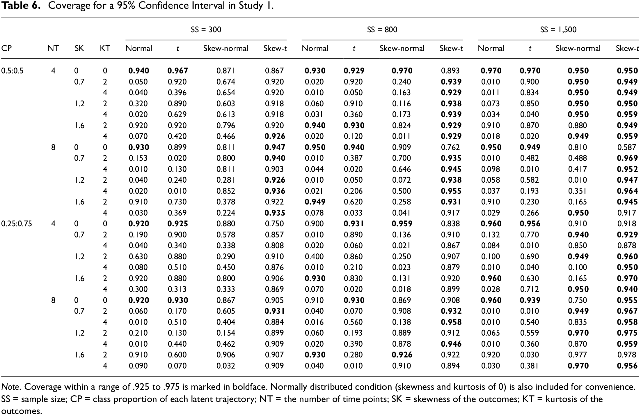
Note. Coverage within a range of .925 to .975 is marked in boldface. Normally distributed condition (skewness and kurtosis of 0) is also included for convenience. SS = sample size; CP = class proportion of each latent trajectory; NT = the number of time points; SK = skewness of the outcomes; KT = kurtosis of the outcomes.
Study 2
In this section, normal distribution is employed like conventional GMMs. Instead, each of two data transformations is used to treat nonnormality. Therefore, Study 2 investigates whether van der Waerden quantile normal scores or adjusted logarithmic transformation produces more accurate parameter estimates. The GMMs are evaluated based on the same four criteria as in Study 1: convergence rate, parameter bias, MSE, and coverage.
Convergence Rate
Generally, the GMMs based on van der Waerden quantile normal scores (VW-GMMs) successfully converge under almost all conditions, with convergence rates that are higher when the sample size is larger (Table 7). The GMMs based on adjusted logarithmic transformation (AL-GMMs) show slightly better convergence rates than the VW-GMMs on average. Indeed, regardless of the simulation design, the AL-GMMs consistently have high-convergence rates.
Convergence Rates in Study 2.

Note. Normally distributed condition (skewness and kurtosis of 0) is also included for convenience. SS = sample size; CP = class proportion of each latent trajectory; NT = number of time points; SK = skewness of the outcomes; KT = kurtosis of the outcomes; VW = van der Waerden quantile normal scores; AL = adjusted logarithmic transformation.
Parameter Bias
As seen in Table 8, the VW-GMMs produce seriously biased parameter estimates. The bias does not fall within the tolerable range of −0.10 to 0.10 (Finch et al., 1997; Kaplan, 1988) for any of the conditions. In more details, larger sample sizes generally led to greater bias except when SS = 300 and CP = 0.5:0.5. In terms of class proportion, the parameter estimates get further biased with unbalanced latent trajectories that led to lower bias just in case SS = 300 and NT = 4. The AL-GMMs produce unbiased estimates for a wider range of conditions, but only four combinations of conditions meet the cut-off criteria regardless of the sample size (CP = 0.5:0.5 NT = 4 SK = 1.2 KT = 2, CP = 0.5:0.5 NT = 4 SK = 1.6 KT = 4, CP = 0.5:0.5 NT = 8 SK = 1.6 KT = 4, and CP = 0.25:0.75 NT = 4 SK = 1.2 KT = 2). The accuracy of the estimates falls slightly when NT = 8 compared with NT = 4 but, if the GMMs have a skewness level of 1.6, a higher number of time points reduces the logit bias. When KT = 2, if the levels of skewness are higher, the bias of the parameter estimates also decreases for SK = 1.2 and then rises again for SK = 1.6.
Bias of the Logit for the Probability of Belonging to Class 1 in Study 2.

Note. The logit for 0.5:0.5 is 0 and for 0.25:0.75 is −1.099. Absolute values lower than 0.1 are marked in boldface. Normally distributed condition (skewness and kurtosis of 0) is also included for convenience. SS = sample size; CP = class proportion of each latent trajectory; NT = the number of time points; SK = skewness of the outcomes; KT = kurtosis of the outcomes; VW = van der Waerden quantile normal scores; AL = adjusted logarithmic transformation.
Mean Square Error
On average, when the ratio of latent trajectories is unbalanced, an increase in the sample size tends to raise the MSE of the VW-GMMs (Table 9). The GMMs with unbalanced class proportion have lower MSE when NT = 4, but if with balanced one, lower MSE is obtained under models including more time points. Kurtosis is more influential factor than skewness to MSE of the VW-GMMs that exhibit larger MSE with higher level of kurtosis. Compared with the VW-GMMs, the MSE is generally lower for the AL-GMMs, apart from a few cases where SK = 1.6 and KT = 2. However, a larger MSE is observed for AL-GMMs with larger sample sizes. AL-GMMs with unbalanced latent trajectories have a slightly higher MSE when NT = 4 except for a few cases. In terms of nonnormality, MSE is lower at SK = 1.2 and then rises at SK = 1.6 on average for KT = 2. At a higher kurtosis level, an increase in skewness reduces the MSE, but this trend weakens if the sample size rises. In contrast to skewness, the kurtosis of the distribution in the outcomes does not have a clear effect on MSE.
Mean Square Error in Study 2.
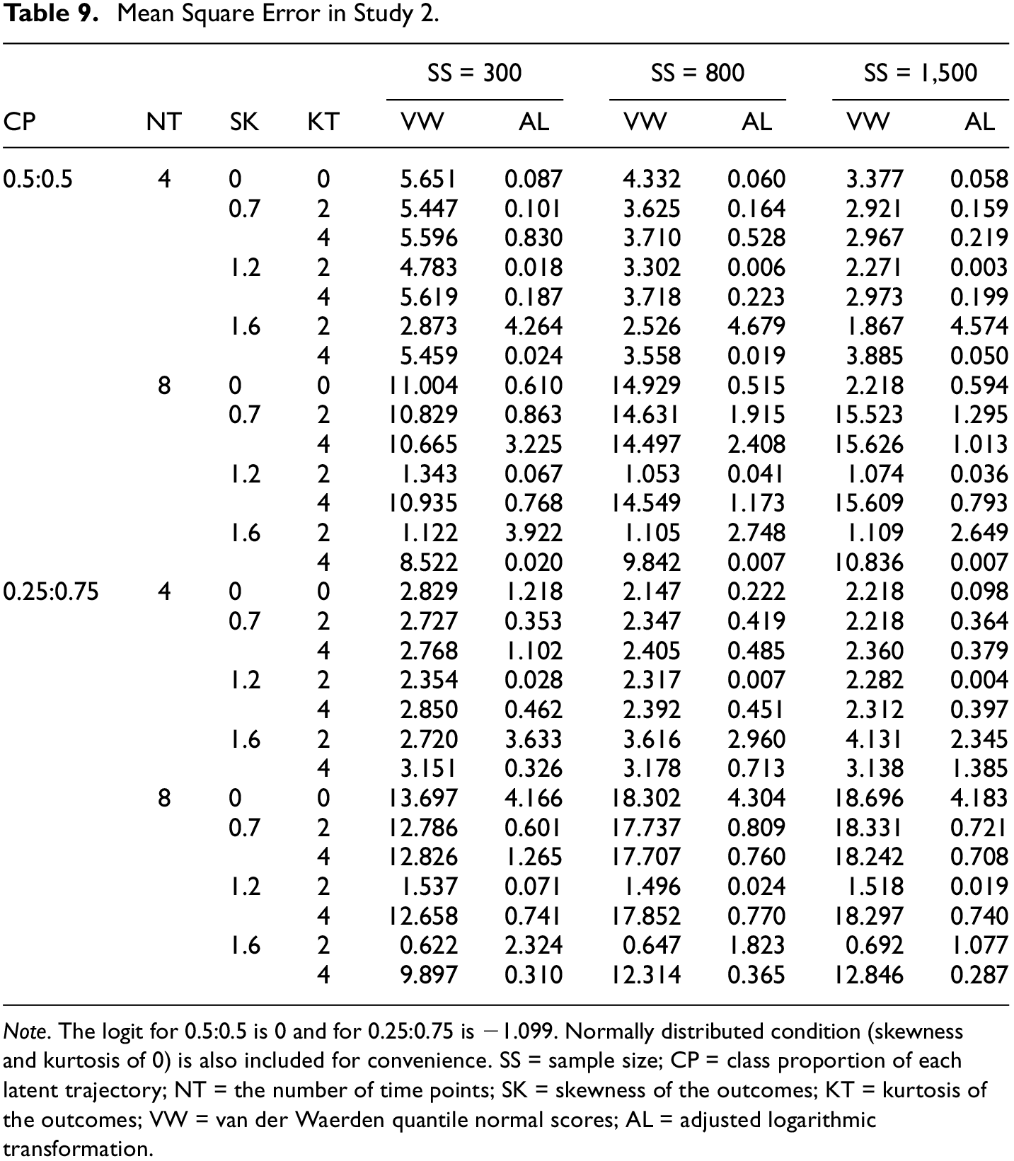
Note. The logit for 0.5:0.5 is 0 and for 0.25:0.75 is −1.099. Normally distributed condition (skewness and kurtosis of 0) is also included for convenience. SS = sample size; CP = class proportion of each latent trajectory; NT = the number of time points; SK = skewness of the outcomes; KT = kurtosis of the outcomes; VW = van der Waerden quantile normal scores; AL = adjusted logarithmic transformation.
Coverage
The VW-GMMs produce the worst coverage for all conditions (Table 10), with a highest value of 0.440 (when SS = 300, CP = 0.5:0.5, NT = 4, SK = 1.6, and KT = 2). However, though the AL-GMMs exhibit better coverage overall, the low number of conditions under which the estimate falls within the range of .925 to .975 (Bandalos, 2006; Muthén & Muthén, 2000) indicates that the coverage is still not sufficient. In fact, the AL-GMMs have a coverage of between .940 and .970 in only five cases.
Coverage of 95% Confidence Interval in Study 2.
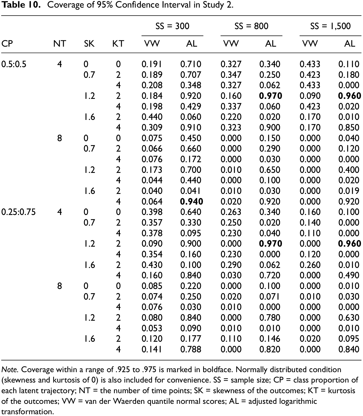
Note. Coverage within a range of .925 to .975 is marked in boldface. Normally distributed condition (skewness and kurtosis of 0) is also included for convenience. SS = sample size; CP = class proportion of each latent trajectory; NT = the number of time points; SK = skewness of the outcomes; KT = kurtosis of the outcomes; VW = van der Waerden quantile normal scores; AL = adjusted logarithmic transformation.
Overall, based on the number of conditions for which all four evaluation criteria (convergence rate, parameter bias, MSE, and coverage) are satisfied or show allowable levels, skew-t GMMs outperform AL-GMMs. For the skew-t GMMs, the number of conditions that satisfy all four criteria increases as the sample size rises. In addition, balanced skew-t GMMs are preferable to their unbalanced counterparts in terms of optimizing the outcomes of all four criteria. The AL-GMMs produce only a single condition where the four evaluation criteria meet the defined standards when the sample size is 300 and only two each for sample sizes of 800 and 1,500, respectively. This means that using the skew-t distribution approach may be more appropriate for accurate parameter estimation regardless of the model structure (e.g., sample size, the subgroup size of each latent trajectory, and the number of outcome variables) and the level of nonnormality in the outcomes (e.g., the skewness and kurtosis).
However, in terms of efficiency, the skew-t GMMs require more computing time in parameter estimation than do the AL-GMMs. This disadvantage has been discussed in previous simulation research (e.g., Muthén & Asparouhov, 2015; Son et al., 2019). Skew-t GMMs are characterized by slower computation than other approaches, particularly for larger sample sizes, because they need to handle raw data in every step (Muthén & Asparouhov, 2015). Similarly, the skew-t GMMs employed in this present study require approximately 25 to 30 minutes for computation, while the AL-GMMs require only about 3 to 5 minutes to compute the estimates, irrespective of the simulation conditions.
An Application to Reading Scores From the ECLS-K Database
This section applied nonnormal linear growth model to the reading scores development over the ages from kindergarten to first grade using the Early Childhood Longitudinal Study–Kindergarten (ECLS-K) class database (National Center for Education Statistics, 1998). As Depaoli et al. (2019) already illustrated how much skewed the reading scores (i.e., repeated measures) were, this study also use these data to show performance of growth modeling under skew-t distribution.
For details of used data in this section, the reading scores were scaled by item response theory across four time points throughout 1998 to 2000 panels of ECLS-K; note that the reading scores were reestimated based on an expanded set of items, all those used in kindergarten through eighth grade. Assessment on children’s reading achievement was conducted in the fall and spring of kindergarten and first grade, respectively, across 18 months. The time intervals between the assessments were not equidistant, so the growth modeling for these data reflected the unequal spacing of waves. For the purpose of this example, missing data were removed. A total sample size of 4,176 children across 18 months (i.e., four time points) was analyzed for nonnormal growth modeling of item response theory -scaled reading scores. Nonnormality of the four repeated measures was shown in Figure 2.

Four time points of reading score histograms. (a) Time 1 (fall 1998). (b) Time 2 (spring 1999). (c) Time 3 (fall 1999). (d) Time 4 (spring 2000).
Following previous literatures (Guerra-Peña & Steinley, 2016; Muthén & Asparouhov, 2015), BICs were compared throughout six approaches (i.e., four types of skew-t family distribution and two normalizing transformations) according to the number of latent class. As a result, in Figure 3, the model using skew-t distribution showed the lowest BIC values among four skew-t family distributions (i.e., the normal, t, skew-normal, and skew-t). This supported the present study and other previous simulation studies (Depaoli et al., 2019; Guerra-Peña & Steinley, 2016; Muthén & Asparouhov, 2015; Son et al., 2019) that relaxing within-class normality assumption and using skew-t as substitute made better performance of GMM for nonnormally distributed data. Additionay, considering a large gap between BIC values of the models (i.e., with one and two latent classes) under the normal growth modeling, it also showed that conventional growth modeling might have high possibility to make spurious classes under nonnormality. Meanwhile, the model under adjusted logarithmic transformation had lower BICs than under van der Wearden quantile normal scores, meaning that adjusted logarithmic transformation performed better under this applied data. This result also echoes the finding of the Study 2 in this article.
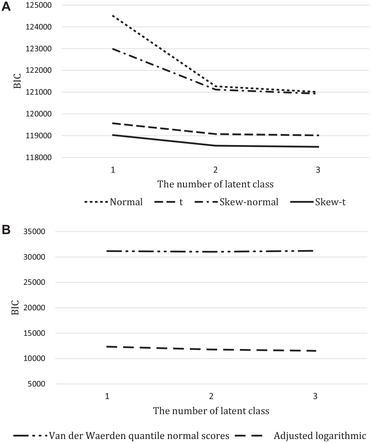
Bayesian information criterion (BIC) of growth modeling for the reading scores. (a) Under four types of skew-t family distribution. (b) Under two types of normalizing transformations.
The model with one latent class was selected according to the BIC results of skew-t and adjusted logarithmic approaches, because BICs of the model with two latent classes were not much different from one latent class. Distinct from this study focusing on the bias of parameter estimates (i.e., bias of logit for probability to belonging to each latent class), only one latent class existed in these reading scores data. So, referring to the approach of exhibiting real data analysis in Depaoli et al. (2019), distance from 50% percentile (i.e., median) of observed scores to estimated growth trajectories was calculated at each time point (see Figure 4). The distance was standardized to make comparison easier, because data transformation including in two models (i.e., adjusted logarithmic and van der Wearden quantile normal scores) made data changed in terms of data scale, unit, and so on. Figure 4 showed that the skew-t modeling generally performed the nearer growth means at each time point. In case of fourth time point, the reading scores were almost normally distributed (see Figure 2 d), so skew-t growth modeling had far distance comparing with others. In contrast to skew-t, the normal and skew-normal modeling produced the nearest growth means only at fourth time point. Meanwhile, both two types of data transformation were shown to have far distance from 50% percentile. Overall, growth modeling for the reading scores from ECLS-K database was well specified with skew-t distribution.
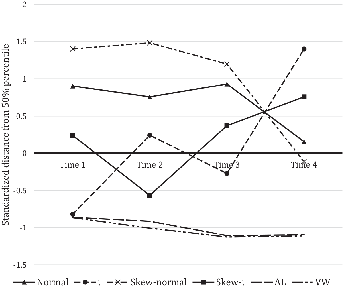
Standardized distance from 50% percentile of data.
Summary
In the present study, five factors were manipulated—sample size (300, 800, and 1,500), the skewness of the outcome variables (0.7, 1.2, and 1.6), the kurtosis of the outcome variables (2 and 4), the number of time points (4 and 8), and the class proportion of each latent trajectory (0.5:0.5 and 0.25:0.75)—and applied to the simulation models in both Study 1 and Study 2 to represent more realistic and diverse data conditions, especially in terms of the degree of kurtosis and the unbalanced class proportion of latent trajectories. In total, 72 simulation conditions (3×3×2×2×2) were generated and 100 replications run for each one. Based on these simulation models, the following summary can be drawn from the results.
First, of the four distributions tested in Study 1, the skew-t distribution was the most appropriate for nonnormal GMMs in terms of obtaining unbiased logits of probability when two subgroups were assumed to exist in the true population. The present study demonstrated that skew-t GMMs produced the most accurate parameter estimates. This finding echoes that of previous simulation studies (see, e.g., Depaoli et al., 2019; Muthén & Asparouhov, 2015; Son et al., 2019). Consistent with Son et al. (2019), in most conditions the absolute bias was less than 0.1, and the MSE was also lower compared with the other three distributions. Additionally, the number of conditions for which the cut-off criteria were met was highest for skew-t GMMs. The skew-t GMMs also obtained much better results in general when the sample size was larger (i.e., SS = 1,500), which supports the results of Depaoli et al. (2019) and Son et al. (2019). As other studies less focused on the extent to which the class proportion affects biases on the estimation, it is a point of significance in this study to find that the skew-t GMMs showed better performance when the class proportion in the population was balanced. Meanwhile, performance of skew-t GMM under normally distributed outcome variables was not bad and vice versa (i.e., normal GMM under nonnormally distributed outcome variables) was not good (see Tables 3–6 for details), which was also similar to the results of Depaoli et al. (2019).
Even with the advantages of using a skew-t distribution in nonnormal GMM, caution is required under certain circumstances. When the sample size is small (see, e.g., Depaoli et al., 2019; Son et al., 2019) and the class proportion of the latent trajectories is unbalanced, the estimates produced by skew-t GMMs may be partially affected by high levels of kurtosis. The MSE can also be higher, and the coverage is unlikely to fall within the range of .925 to .975. Furthermore, it should be noted that the convergence rate of skew-t GMMs falls as the nonnormality level increases when there are unbalanced latent class sizes. Consistent with the results of Depaoli et al. (2019), fitting the model to a skew-t distribution requires much greater computational resources than other distributions (i.e., the normal or t in this article). Nevertheless, in terms of the overall results, skew-t GMMs may prove useful for obtaining accurate parameter estimates when the outcome variables follow a nonnormal distribution.
Second, the performance of the models based on adjusted logarithmic transformation was generally better than that of the models based on van der Waerden quantile normal scores. The AL-GMMs consistently produced high rates of convergence regardless of the simulation design. Compared with VW-GMMs, more conditions produced unbiased estimates, smaller MSEs, and allowable coverage when using AL-GMMs.
Third, adopting a skew-t distribution as an approach to nonnormal GMM can be recommended for two primary reasons. First, the skew-t GMMs overwhelmingly outperformed the AL-GMMs, with much more accurate estimation and greater robustness under various simulated conditions. Second, the results arising from data transformation approaches (e.g., the mean and variance of the intercept and slope) are known to be difficult to interpret (Agresti & Finlay, 2009). The computational efficiency of AL-GMMs may not compensate for this issue of unclear interpretation.
Discussion
By investigating more diverse simulation conditions that better reflect real-life data sets, it is expected that the present study will offer useful guidelines for applied researchers in social science when approaching nonnormal GMM. The main implications of this simulation study are as follows.
First, this article demonstrated that the most accurate parameter estimation comes from skew-t GMMs, which supports the findings of previous simulation studies (see, e.g., Depaoli et al., 2019; Muthén & Asparouhov, 2015; Son et al., 2019), although one main difference exists in terms of modeling nonnormality, which comes from manifest variables not latent growth factors (i.e., this article dealt with nonnormally distribution of manifest variables, while three articles did of latent growth factors). Most results of this simulation study share that of the previous ones in terms of better performance of skew-t GMM under larger sample size (Depaoli et al., 2019; Son et al., 2019), greater computing time for skew-t GMM (Depaoli et al., 2019), and so on. So, one of implications in this article was made by considering different levels of kurtosis in the repeated measures of the model and more practical conditions for class proportion. This study attempted to examine the performance of skew-t GMMs over a wider range of data in terms of estimation accuracy, particularly for the logit of probability, thus expanding on previous research related to biased parameter estimates caused by nonnormality in GMM. It was newly revealed that a high degree of kurtosis in the distribution of outcomes and unbalanced subgroup sizes can reduce the accuracy of skew-t GMMs.
Second, the applicability of data transformation to nonnormal GMM was investigated. Although a few normalizing methods have been tested using other mixture models, such as LPA, no previous research has investigated data transformation in nonnormal GMM simulations. This article focused on two methods (i.e., adjusted logarithmic transformation and van der Waerden quantile normal scores) proposed by other studies and found that adjusted logarithmic transformation may be more appropriate for nonnormal repeated measures in GMM than van der Waerden quantile normal scores. Specifically, it was contrast to nonnormal LPA of Morgan et al. (2016), van der Waeden quantile normal scores produced not accurate parameter estimates under nonnormal GMM. This difference might come from whether the growth factors are modeled or not. Meanwhile, it was similar to Kupek (2005) in terms of suitability of log-linear transformation within SEM framework. But there is a big difference between this article and Kupek (2005) on the aim of normalization. Contrary to the study of Kupek (2005) where binary variables were normalized for linearization, this article focused on nonnormally distributed outcomes. Additionally, the modeling approach to outcomes (i.e., longitudinal or not) in this article is also distinct from Kupek (2005), so this simulation study had an implication with examining appropriateness of the logarithm transformation on nonnormal GMM.
Third, this study compared the performance of alternative distribution approaches (i.e., the skew-t GMMs) with that of data transformation approaches (i.e., the AL-GMMs). It was found that fitting a model to normalized outcomes can reduce computation time, but it does not guarantee accurate parameter estimates or interpretable results. Therefore, this study offers guidelines for applied researchers in terms of which approach is more suitable when repeated measures in GMM follow a nonnormal distribution (i.e., in this article, most evaluation criteria recommended skew-t GMMs than AL-GMMs under various nonnormality of outcomes).
As with any Monte Carlo simulation study, these findings and implications are generalizable only for the conditions examined in this study. Even though the chosen design factors and the manipulated conditions are based on previous empirical research, the results may not be directly applicable to every situation because not all cases were covered by the results of this study. As such, this article has certain limitations and associated recommendations for future research that should be noted.
First, future research needs to expand on the findings of the present study by considering other conditions not included in this simulation design but that are characteristic of real data. For example, the kurtosis of the distribution of repeated measures may be increased to cover more extreme cases of nonnormality (e.g., adolescent alcohol use, which had a skewness of 1.99 to 10.69 in D’Amico et al., 2016). Only two levels of kurtosis were manipulated in this study, so assessing higher levels of kurtosis can provide insight and implications. Additionally, this article focused on only positively skewed data, so it should be cautious to apply the results of this article to other situations such as negative skewness. Future research might back up this point by considering various types of skewed data.
Second, it would be helpful if the analyzed GMMs were more complicated. For instance, only two latent classes were assumed in this study. Future research can include more subgroups within the true population (e.g., three or four classes, which is a common occurrence in applied research). Additionally, the latent growth factors may consist of higher order terms such as quadratic or cubic functions to more precisely track the developmental path of the variable of interest.
Third, class enumeration in nonnormal GMM should be thoroughly reviewed with the occurrence issue of parameter bias. Correctly deciding on the number of latent classes is also important for researchers because this number may not be known a priori. In the present study, a comparison of parameter bias for the four distribution types and for the data transformation approaches was highlighted. Even though Muthén and Asparouhov (2015) demonstrated that skew-t GMMs can detect the correct number of latent classes when exploring the results of BIC under nonnormal data, other indices or likelihood ratio tests (e.g., AIC, SBIC, LMR-LRT, BLRT, etc.) also need to be examined with respect to skew-t GMMs that involve nonnormal outcomes.
In conclusion, the findings of this study are expected to help researchers gain confidence in selecting the most appropriate approach for nonnormal outcome variables in growth mixture modeling.
Footnotes
Declaration of Conflicting Interests
The author(s) declared no potential conflicts of interest with respect to the research, authorship, and/or publication of this article.
Funding
The author(s) received no financial support for the research, authorship, and/or publication of this article.
