A Monte Carlo Study of Confidence Interval Methods for Generalizability Coefficient

Abstract

Computing confidence intervals around generalizability coefficients has long been a challenging task in generalizability theory. This is a serious practical problem because generalizability coefficients are often computed from designs where some facets have small sample sizes, and researchers have little guide regarding the trustworthiness of the coefficients. As generalizability theory can be framed to a linear mixed-effect model (LMM), bootstrap and simulation techniques from LMM paradigm can be used to construct the confidence intervals. The purpose of this research is to examine four different LMM-based methods for computing the confidence intervals that have been proposed and to determine their accuracy under six simulated conditions based on the type of test scores (normal, dichotomous, and polytomous data) and data measurement design (p×i×r and p× [i:r]). A bootstrap technique called “parametric methods with spherical random effects” consistently produced more accurate confidence intervals than the three other LMM-based methods. Furthermore, the selected technique was compared with model-based approach to investigate the performance at the levels of variance components via the second simulation study, where the numbers of examines, raters, and items were varied. We conclude with the recommendation generalizability coefficients, the confidence interval should accompany the point estimate.

Keywords

generalizability bootstrap linear mixed-effect model confidence interval standard error

Introduction

Generalizability theory (G-theory) provides a conceptual framework and statistical procedures for evaluating the reliability of behavioral measurements such as test scores, performance evaluations, and survey ratings (Cronbach et al., 1963). A key feature of G-theory is that it allows the researcher to quantify the contribution of different sources of variance to overall measurement error. In assessment situations, common sources of variance include facets such as the particular sample of test questions the examinee responds to, the raters who evaluated those questions, the types of rating scales that were used, and the particular occasion under which the observations were obtained (Brennan, 2001; Shavelson & Webb, 1981). G-theory relies on analysis of variance techniques to partition test scores into the sources of variance that contribute to those scores. Variance components are estimated for each facet and are used as the basis for constructing indices of measurement error and score reliability. Once researchers understand sources of measurement error, they can make informed decisions to fine tune their measurement procedures (e.g., increase the number of test questions; decrease the number of raters).

One of the more common indices in G-theory is the generalizability coefficient, designated as rho-square (ρ²). Under certain conditions (e.g., a group of students responding to a sample of test questions), the generalizability index is analogous to Cronbach’s coefficient alpha (Brennan, 2001; Shavelson & Webb, 1981) and is often interpreted as a fixed-point estimate. However, in the absence of confidence intervals (CIs), a point estimate of generalizability coefficient can be misleading. To illustrate, in the field of medical education, a type of performance test known as an objective structured clinical examinations (OSCEs) is often used for evaluating medical students’ readiness for practice. G-theory is typically used to evaluate the quality of ratings from an OSCE, and the generalizability coefficient is the primary evidence for either accepting or modifying the exam administration procedures. If the point estimate of the generalizability coefficient is 0.85 where the 95% CI spans from 0.65 to 0.90, the decision makers may not be satisfied with the current procedures, assuming the minimum acceptable value is 0.70. Therefore, knowing CIs around a generalizability coefficient is practically beneficial for well-grounded evaluations.

Researchers have proposed methods for estimating CIs (or standard errors) of the variance components and generalizability coefficients obtained in G-theory (Brennan, 2006; Feldt, 1965). These methods can be classified as either model-based or empirically based. Model-based methods assume that scores are randomly, independently, and normally distributed (iid), while resampling relies on bootstrap or simulation techniques (Brennan, 2006, 2007; Brennan et al., 1987; Gao & Brennan, 2001; Moore, 2010; Othman, 1995; Tong & Brennan, 2006, 2007). The former requires complex mathematical deriving and, so far, have been developed only for straightforward measurement designs (e.g., p×i) but not for nested designs, for example (p× [i:r]; Almehrizi, 2020). Although the latter methods are straighforward to implement, selecting different bootstrap or simulation techniques as well as tuning their corresponding configurations (e.g., the facet sampled; number or sizes of the samples) often result in inconsistent results that can be challenging to reconcile. For instance, Tong and Brennan (2007) show that bootstrapping from person and item perspectives produce large discrepancies in CIs.

The purpose of the present study is to evaluate the effectiveness of various resampling methods for estimating standard errors and CIs in generalizability theory. We focus on resampling methods because they are likely to be accessible researchers and users, and are applicable to a broad range of measurement designs. This study builds on the work of Tong and Brennan (2007) by adapting new approaches from linear mixed-effect model (LMM) paradigm, such that the performance of the corresponding CIs can be investigated.

The resampling methods are based on a two-step cycle where the “resampling” strategy is followed with the step of “estimating” models. For example, a new data set sampled (i.e., bootstrapped) from the original data set is fed into a G-theory model, and model parameter estimates, as well as relevant statistics calculated from the estimates, are recorded and aggregated. This iterative, two-stage process continues until a vector of the statistic of interest is formed. There are multiple computational algorithms for estimating variance components from G-theory. The more common methods include: analysis of variance using expected mean square (EMS) equations (Cornfield & Tukey, 1956); Henderson’s Method 1 and Method 3 (Henderson, 1953); minimum norm quadratic unbiased estimation (Rao, 1970). More recent approaches rely on maximum likelihood (ML) estimation, including full information ML for handling missing data and unbalanced designs, as well as restricted maximum likelihood (REML) within a LMM framework. LMMs, also known as a hierarchical linear models or as multilevel modeling, subsumes a class of statistical models specified for analyzing designs with clustering or nested structures (Raudenbush & Bryk, 2002) well suited for many complex measurement designs. Modeling in G-theory can be viewed as an instance of building an LMM according to a G-theory design (Brennan, 1992). Jiang (2018) adopted a software package called lme4 (Bates et al., 2015), a library specifically for analyzing LMMs in the R program (R Core Team, 2021) to handle variance component estimation in G-theory; similar works can be found in Huebner and Lucht (2019). The present article follows Jiang’s (2018) approach to variance component estimation, and uses bootstrap and simulation techniques from LMM paradigm to construct CIs around generalizability coefficients.

The bootstrap and simulation techniques from LMM paradigm are not identical to the traditional resampling strategy. Instead of resampling from the original responses, many LMM bootstrap and simulation techniques first estimate the model, and then use the model to generate new data sets that are further fed to the same model. At each iteration, feeding models with fresh data points produces a set of new parameter estimates. As a set of the parameter estimates can be used to obtain a generalizability coefficient, M sets of the parameters estimates can produce M generalizability coefficients for constructing CIs.

In this article, four mainstream LMM-based techniques are selected for evaluation: (1) parametric bootstrap (PB), (2) semiparametric bootstrap (SPB), (3) nonparametric bootstrap (NPB), and (4) posterior simulation (PS). To demonstrate the differences among the techniques, it is necessary to define the terms of LLMs. If Y is a response column matrix with n rows (i.e., a vector), an LLM can be expressed as:

Y = X β + Zb + ε, where b ~ N (0, G) and ε ~ N (0, R)

where $X$ is an n by k covariate matrix (where k is the number of fixed effects), $Z$ is an n by m random-effect matrix (m is the number of random effects), G is the variance–covariance matrix of the random effects of dimension m by m, and finally, R is the variance–covariance matrix of the errors, which in many situations is assumed to be iid (i.e., $R$ = $σ^{2} I$ where $I$ is an identity matrix). $β$ is the fixed-effects vector and $b$ is the random-effects vector.

PB: (1) Fit the original LMM to the data to obtain the $\hat{β}$ , $\hat{G}$ , and $\hat{R}$ . (2) Generate the bootstrap samples via the fitted model $Y^{*} = X \hat{β} + Z {\hat{b}}^{*} + {\hat{ε}}^{*}$ , where ${\hat{b}}^{*}$ and ${\hat{ε}}^{*}$ are generated from $N (0, \hat{G})$ and $N (0, \hat{R})$ , respectively. (3) Fit the original LMM to the bootstrap data and obtain ${\hat{β}}^{*}, {\hat{G}}^{*}$ , and ${\hat{R}}^{*}$ . (4) Repeat Steps 1 to 3.

SPB: (1) Fit the original LMM to the data to obtain the $\hat{β}$ , $\hat{G}$ , and $\hat{R}$ . (2) Obtain residuals via $\hat{ε} = Y - X \hat{β}$ . (3) Draw a sample size of m with replacement from these residuals and denote them by ${\hat{ε}}^{*}$ . (4) Construct the bootstrap data set using the fitted model $Y^{*} = X \hat{β} + {\hat{ε}}^{*}$ . (5) Fit the LMM to the bootstrap data and obtain ${\hat{β}}^{*}, {\hat{G}}^{*}$ , and ${\hat{R}}^{*}$ . (6) Repeat Steps 1 to 5.

NPB: (1) Match $y$ and $X$ to form new sets of ( $y$ , $X$ ). (2) Draw a sample of size m with replacement from the m pairs and denote them by ( $Y^{*}$ , $X^{*}$ ). (3) Fit the original LMM to the bootstrap data and obtain ${\hat{β}}^{*}, {\hat{G}}^{*}$ , and ${\hat{R}}^{*}$ . (4) Repeat Steps 1 to 3.

PS: (1) Fit the original LMM to the data to obtain the $\hat{β}$ , $\hat{G}$ , and $\hat{R}$ . (2) Simulate $σ^{*} = \hat{σ} \sqrt{(n - k) / ω}$ , where $ω$ is a random draw from the $χ^{2}$ distribution with n−k degrees of freedom. (3) Given the random draw of $σ$ , simulate ${\hat{β}}^{*}$ from a multivariate normal distribution with mean $\hat{β}$ and $σ^{*^{2}} I$ . (4) Simulate ${\hat{G}}^{*}$ with a similar fashion and repeat all steps.

To summarize without the mathematical terms, PB utilizes the initial LMM to generate new data points that are further used to construct models, such that multiple sets of parameter estimates for each effect can be obtained. SPB is akin to PB except that the data generation process does not rely on the initial LMM but rather on a fixed-effect model rebuilt from the LMM’s residuals. NPB draws rows from the original data sets to form a new data set, estimate a new model with the data set, and repeat the process. PS derives posterior distributions for each parameter and samples from the distributions to form sets of parameter estimates. More details regarding PB to PS can be found in Davison and and Hinkley (1997), Gelman and Hill (2006), as well as Shang and Cavanaugh (2008).

Method

This study consists of two simulation studies, while the first one investigates CIs at the level of generalizability coefficient and the second one further examines CIs at the variance component level with references. The first one follows the general design of the simulation study conducted by Tong and Brennan (2007). The data generation process was completed [or conducted, or executed] for normal, dichotomous, and polytomous responses. The sample sizes were set to $n_{p}$ = 100, $n_{i}$ = 20, and $n_{r}$ = 2 where the subscripts p, i, and r represented the facets of persons, items, and raters, respectively. Two commonly seen designs, p×i×r and p× [i:r], were adopted. The former is a fully crossed data collection design where all examinees respond to all 20 items, which are then rated the same two raters. The latter is a nested design in which some items are nested within raters.

For normal data, responses for the p×i×r design were generated on the basis of Equations 1 and 2. Equation 1 shows that an observed score, $Y_{pri}$ , for person p on item i rated by rater r is made of the grand mean $μ$ , person effect $v_{p}$ , item effect $v_{i}$ , rater effect $v_{r}$ , interaction terms of any two random effects, and error effect $ϵ_{pi}$ . Correspondingly, the relevant variance components are outlined in Equation 2. All $σ$ s are dispersion parameters from independent and identically distributed (iid) normal shapes whose central locations are all 0, for example, $v_{p} ~ N (0, σ_{p}^{2})$ , $v_{i} ~ N (0, σ_{i}^{2})$ , and $ϵ_{pi} ~ N (0, σ_{pi . e}^{2})$ .

Y_{pri} = μ + v_{p} + v_{i} + v_{r} + v_{pi} + v_{ir} + v_{pr} + ϵ_{pri},

(1)

σ {(Y)}_{pri}^{2} = σ_{p}^{2} + σ_{i}^{2} + σ_{r}^{2} + σ_{pi}^{2} + σ_{ir}^{2} + σ_{pr}^{2} + σ_{pri . e}^{2} .

(2)

Similarly, observed scores and variances for the p× [i:r] design were generated using Equations 3 and 4.

Y_{pir} = μ + v_{p} + v_{r} + v_{i : r} + v_{pr} + ϵ_{pi : r},

(3)

σ {(Y)}_{pir}^{2} = σ_{p}^{2} + σ_{r}^{2} + σ_{i : r}^{2} + σ_{pr}^{2} + σ_{pi : r}^{2} .

(4)

For dichotomous data, Equations 1 to 4 were again used for the two designs, respectively. If the simulated score exceeded 1, a response of 1 was assigned; otherwise, a response of 0 was assigned to create dichotomous responses. As the parameter values for variance components for dichotomous data were not readily available in the simulation process, 5000 data sets were produced and their $σ^{2}$ estimates were recorded and averaged to serve as the true parameter values.

For polytomous data, the normal distributions in Equations 2 and 4 were replaced by binominal distributions. To illustrate, $v ~ B (a, b)$ can sample a binomial value for $a$ trials with the probability of success being $b$ . The distributional settings in Gao and Brennan (2001) as well as Lane et al. (1996) were used for the p×i×r and the p× [i:r] designs, respectively. That is, in the p×i×r design, B(2, 0.7966), B(1, 0.8570), B(1, 0.98785), B(2, 0.7313), B(1, 0.98579), B(1, 0.9975), and B(2, 0.8025) were specified for person, item, rater, person and item interaction, person and rater interaction, rater and item interaction, and error effects, respectively. On the other hand, in the p× [i:r] design, B(1, 0.713), B(1, 0.843), B(2, 0.713), B(1, 0.930), and B(5, 0.6300) were specified for person, rater, item (nested within raters), person and rater interaction, and error effects, respectively. The scores ranged from 0 to 10 for each item in both designs. The true parameter values for $σ^{2}$ were obtained from the way identical to that of for dichotomous data. The true parameters used to generate data sets are listed in Table 1.

Table 1.

True Parameters for the Simulation Study.

	p×i×r				p× [i:r]
	Normal	Dichotomou	Polytomous		Normal	Dichotomou	Polytomous
$σ_{p}^{2}$	16.0000	0.0109	0.3241	$σ_{p}^{2}$	16.0000	0.0108	0.2046
$σ_{i}^{2}$	4.0000	0.0028	0.1270	$σ_{i : r}^{2}$	7.0000	0.0048	0.4093
$σ_{r}^{2}$	1.0000	0.0007	0.0120	$σ_{r}^{2}$	1.0000	0.0006	0.1324
$σ_{pi}^{2}$	64.0000	0.0449	0.3930	Na	/	/	/
$σ_{ir}^{2}$	3.0000	0.0021	0.0025	Na	/	/	/
$σ_{pr}^{2}$	2.0000	0.0014	0.0140	$σ_{pr}^{2}$	2.0000	0.0014	0.0651
$σ_{pri . e}^{2}$	144.0000	0.1873	0.3170	$σ_{pi : r . e}^{2}$	208.000	0.2323	1.1655
$σ_{Δ}^{2}$	8.5750	0.0081	0.0470	$σ_{Δ}^{2}$	6.8750	0.0070	0.1381
$E ρ_{Δ}^{2}$	0.6511	0.5737	0.8733	$E ρ_{Δ}^{2}$	0.6995	0.6067	0.5970

Note. Na = not applicable.

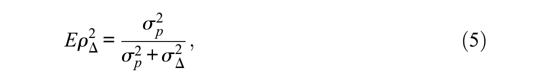
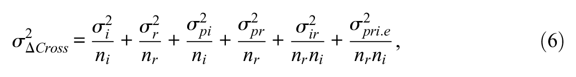
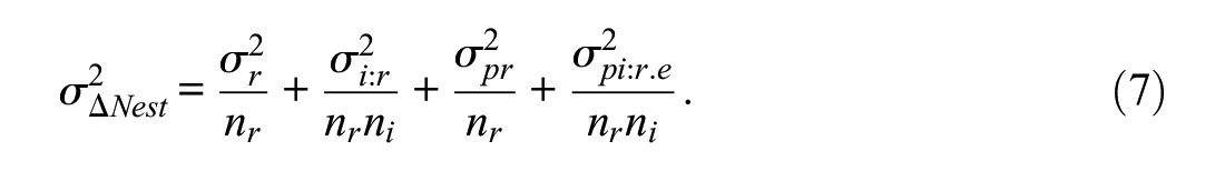
After obtaining true parameter values of variance components by either directly copying from the original values or averaging the simulated values, the true generalizability coefficient can be calculated using Equations 5 to 7. Note that $σ_{Δ}^{2} s$ for two designs were named to $σ_{Δ Cross}^{2}$ and $σ_{Δ Nest}^{2}$ , and the generalizability coefficient $E ρ_{Δ}^{2}$ corresponds to absolute error, instead of relative error.¹

E ρ_{Δ}^{2} = \frac{σ_{p}^{2}}{σ_{p}^{2} + σ_{Δ}^{2}},

(5)

σ_{Δ Cross}^{2} = \frac{σ_{i}^{2}}{n_{i}} + \frac{σ_{r}^{2}}{n_{r}} + \frac{σ_{pi}^{2}}{n_{i}} + \frac{σ_{pr}^{2}}{n_{r}} + \frac{σ_{ir}^{2}}{n_{r} n_{i}} + \frac{σ_{pri . e}^{2}}{n_{r} n_{i}},

(6)

σ_{Δ Nest}^{2} = \frac{σ_{r}^{2}}{n_{r}} + \frac{σ_{i : r}^{2}}{n_{r} n_{i}} + \frac{σ_{pr}^{2}}{n_{r}} + \frac{σ_{pi : r . e}^{2}}{n_{r} n_{i}} .

(7)

Each of the p×i×r and the p× [i:r] designs involved 1,000 replications. That said, 1,000 arrays of size 100 × 20 × 2 were generated. For each of the bootstrap techniques, 500 bootstrapping samples were drawn within each of the 1,000 replications. Within each replication, a 95% CI was constructed and the true generalizability coefficient was investigated to see if it was covered within that CI. The primary outcome measure is the coverage rate, which is defined as the proportion of replications that a CI contains the true generalizability coefficient. A secondary outcome is the mean standard deviation of the generated generalizability coefficients from the resampling techniques (i.e., the average dispersion of the resampled statistics).

The second simulation study (1) varies the facet levels of a fully crossed design to create different conditions, (2) utilizes the best technique from the four candidates, (3) calculates the coverage rate as the first simulation study yields, and (4) compares its variance component estimates with a model-based approach based on Satterthwaite’s solution (Smith, 1982). Specifically, the sample sizes were set to $n_{p}$ = [50, 200, 500], $n_{i}$ = [5, 15, 30], and $n_{r}$ = [3,5]; these levels were set to be fully crossed, resulting in 18 conditions in total. Only the coverage rate was used to measure the outcome for the comparative purposes.

Results

Table 2 contains the coverage rates of the first simulation study. To illustrate, the first cell in the table (0.9516) indicates that for continuous (normal) data, the true generalizability coefficient for the p×i×r design was covered by the CIs produced by PB about 95% of the time. It is apparent from Table 2 that PB outperformed the other three methods in all conditions. However, for polytomous response data, the coverage rates for PB dropped, particularly for the p× [i:r] design where coverage rates fell to about 81%. However, all methods performed less well with polytomous data, with huge decrements for methods SPB, NPB, and PS. In general, neither SPB, NPB, or PS was practically trustable as their coverage rates were far below 0.95, leaving a firm belief that these CIs were either drifted far from the target or spanned overly narrow ranges.

Table 2.

Coverage Rates of the Simulated Confidence Intervals (CIs) for Each Simulated Condition.

		Method for computing CIs
Design	Type of scale	PB	SPB	NPB	PS
p×i×r	Continuous	0.9516	0.6150	0.2567	0.0533
	Dichotomous	0.9522	0.8239	0.6090	0.0418
	Polytomous	0.9164	0.1900	0.0650	0.0475
p× [i:r]	Continuous	0.9577	0.8263	0.8592	0.4601
	Dichotomous	0.9615	0.8308	0.8231	0.3308
	Polytomous	0.8101	0.3038	0.2753	0.3734

Note. PB = parametric bootstrap; SPB = semiparametric bootstrap; NPB = nonparametric bootstrap, PS = posterior simulation.

The average standard deviations are listed in Table 3 showing the variability of the coefficients resampled by the selected methods. Consistently, generalizability indices generated by PB spanned a wider range than those of other methods. These findings support the reasoning that the CIs for methods SPB, NPB, and PS were too narrow such that the true generalizability coefficient was left out of the range in many replications. The average standard deviations were larger for the p× [i:r] design than for the p×i×r design.

Table 3.

Mean Standard Deviations of Generalizability Coefficients Across Simulated Conditions.

		Method for computing CIs
Design	Type of scale	PB	SPB	NPB	PS
p×i×r	Continuous	0.0590	0.0326	0.0261	0.0186
	Dichotomous	0.0766	0.0559	0.0484	0.0206
	Polytomous	0.0127	0.0040	0.0028	0.0046
p× [i:r]	Continuous	0.0923	0.0895	0.0902	0.0320
	Dichotomous	0.1293	0.1253	0.1282	0.0346
	Polytomous	0.0946	0.0450	0.0430	0.0575

Note. PB = parametric bootstrap; SPB = semiparametric bootstrap; NPB = nonparametric bootstrap, PS = posterior simulation.

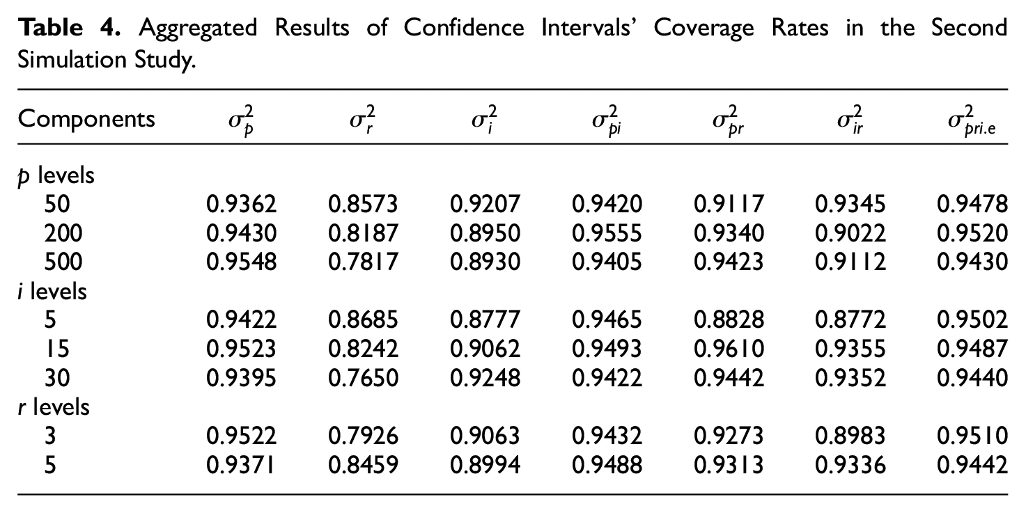
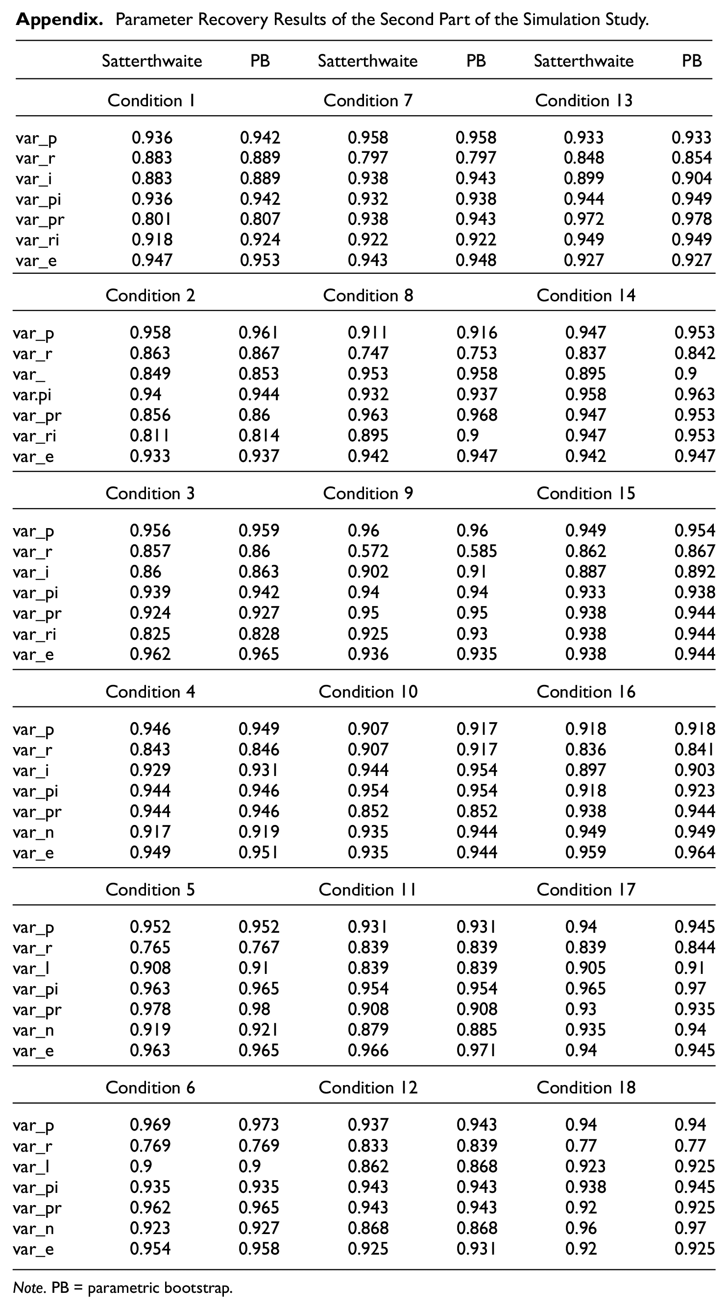
The complete results of the second simulation study are listed in the appendix. As PB outperformed other methods, it was used to compared with Satterthwaite’s approach. In all conditions, the coverage rates yield by PB are slightly higher than those by Satterthwaite’s approach: The differences across all random effect components are less than 0.01. It concludes that, in addition to generating appropriate CIs for generalizability coefficient, PB can reproduce the accuracy yielded by model-based approaches at the levels of variance components; this emphasizes the advantages of the proposed approach over model-based approaches: the capacity of producing accurate CIs at both levels.

Given the statistics produced by Satterthwaite’s approach and PB are extremely similar, PB results are used here to describe the variability of the CIs in different conditions. On average, the coverage rates for $σ^{2}$ =[ $σ_{p}^{2}, σ_{i}^{2}, σ_{r}^{2}, σ_{pi}^{2}, σ_{ir}^{2}, σ_{pr}^{2}, σ_{pri . e}^{2}$ ] are [0.9447, 0.9028, 0.8192, 0.9460, 0.9159, 0.9293, 0.9476]. The CIs for $σ_{r}^{2}$ are much less than 0.95, indicating that low facet levels (only 3 and 5 raters within the simulated conditions) are detrimental to the CIs estimates. Grouping the independent variables, Table 4 aggregates the results at person, item, and rater levels. Interesting findings are outlined as: (1) CIs for $σ_{p}^{2}$ are consistently accurate, even at the conditions of 50 examinees, (2) increasing the number of samples at other facets can be harmful to the facet with smaller sample sizes (e.g., the decremental tendencies in the column of $σ_{r}^{2}$ of Table 4), and (3) increasing the number of samples at a targeted facet can improve CIs’ accuracy of the facet. With the decomposition, it can be seen that, overall the resampling of PB is reliable at a lower level (i.e., variance components) and therefore leads to a trustable CIs for generalizability coefficient.

Table 4.

Aggregated Results of Confidence Intervals’ Coverage Rates in the Second Simulation Study.

Components	$σ_{p}^{2}$	$σ_{r}^{2}$	$σ_{i}^{2}$	$σ_{pi}^{2}$	$σ_{pr}^{2}$	$σ_{ir}^{2}$	$σ_{pri . e}^{2}$
p levels
50	0.9362	0.8573	0.9207	0.9420	0.9117	0.9345	0.9478
200	0.9430	0.8187	0.8950	0.9555	0.9340	0.9022	0.9520
500	0.9548	0.7817	0.8930	0.9405	0.9423	0.9112	0.9430
i levels
5	0.9422	0.8685	0.8777	0.9465	0.8828	0.8772	0.9502
15	0.9523	0.8242	0.9062	0.9493	0.9610	0.9355	0.9487
30	0.9395	0.7650	0.9248	0.9422	0.9442	0.9352	0.9440
r levels
3	0.9522	0.7926	0.9063	0.9432	0.9273	0.8983	0.9510
5	0.9371	0.8459	0.8994	0.9488	0.9313	0.9336	0.9442

Discussion

In a simulation of this kind, a coverage rate of 0.95 indicates an ideal approximation of the 95% CI. In all conditions, PB came closer to 95% than all other methods, while PS was the least accurate. When data responses were normal or dichotomous, it seems appropriate to use PB to obtain CIs for the estimated generalizability coefficients for the two types of designs studied here. Methodologically, PB mimics LMM’s properties to a maximal degree such that the resampling process is based on a structure consistent with the original mode. SPB does not integrate the random-effect components when performing bootstrapping and leaves the part of the information unused. NPB operates bootstrap techniques from the data side, instead of the modeling perspective; therefore, the unsatisfactory results were consistent with the findings in Tong and Brennan (2007). Finally, PS simulates parameters directly from posterior distributions, of which the dispersions seemed to be too conservative compared with other methods.

Most studies that have examined CIs or standard errors within the context of G-theory have focused on the variance components (e.g., Brennan, 2006, 2007; Tong & Brennan, 2007; Wiley, 2000), while this article addresses the issue from the level fo actual generalizability coefficients that aare computed from the variance components. Although there may be some risk in ignoring variance-level CIs, investigating CIs at the level of generalizability coefficients is desirable. One reason is that CIs for variance components do not directly inform the uncertainty of generalizability coefficients, as they cannot be converted to one another via simple or closed-form solutions. In addition, variance components are not by themselves useful for decision-making purposes, while generalizability coefficients are often interpreted as direct evidence for decision making. Also, Cronbach’s $α$ —a reliability coefficient within classical test theory framework—has been extensively studied in terms of its CIs (e.g., Bonett, 2002; Feldt, 1965; Hakstian & Whalen, 1976; Iacobucci & & Duhachek, 2003; Koning & Franses, 2003; Maydeu-Olivares et al., 2007), and the importance of investigating uncertainty applies to generalizability coefficients as well. Note that the computation of the relative generalizability coefficient in a one-faceted is essentially the estimation of Cronbach’s $α$ ; accordingly, CI estimation approaches proposed for Cronbach’s $α$ can be applied to the special form of the G-theory design (see, e.g., Bonett & Wright, 2015; Feldt, 1965; Padilla et al., 2012; Van Zyl et al., 2000; Yuan et al., 2003).

Although Bayesian methods have been used in G-theory (Jiang & Skorupski, 2018; LoPilato et al., 2015), they were not addressed here for two reasons. First, Bayesian methods can be highly sensitive to prior distributions, leading a simulation design less controllable when varying the prior distributions becomes necessary. Second, Bayesian methods are computationally expensive and less used in practice.

Conclusions

G-theory provides an important framework for evaluating the quality of ratings and scores in performance testing. Point estimates of generalizability coefficients are not sufficient because the imprecision of those estimates is unknown to decision makers. The PB technique illustrated here appears to provide one useful way for evaluating the trustworthiness of generalizability coefficients, thus allowing decisions about a test’s design to be made with greater accuracy and confidence.

Footnotes

Appendix

Appendix.

Parameter Recovery Results of the Second Part of the Simulation Study.

	Satterthwaite	PB	Satterthwaite	PB	Satterthwaite	PB
	Condition 1		Condition 7		Condition 13
var_p	0.936	0.942	0.958	0.958	0.933	0.933
var_r	0.883	0.889	0.797	0.797	0.848	0.854
var_i	0.883	0.889	0.938	0.943	0.899	0.904
var_pi	0.936	0.942	0.932	0.938	0.944	0.949
var_pr	0.801	0.807	0.938	0.943	0.972	0.978
var_ri	0.918	0.924	0.922	0.922	0.949	0.949
var_e	0.947	0.953	0.943	0.948	0.927	0.927
	Condition 2		Condition 8		Condition 14
var_p	0.958	0.961	0.911	0.916	0.947	0.953
var_r	0.863	0.867	0.747	0.753	0.837	0.842
var_	0.849	0.853	0.953	0.958	0.895	0.9
var.pi	0.94	0.944	0.932	0.937	0.958	0.963
var_pr	0.856	0.86	0.963	0.968	0.947	0.953
var_ri	0.811	0.814	0.895	0.9	0.947	0.953
var_e	0.933	0.937	0.942	0.947	0.942	0.947
	Condition 3		Condition 9		Condition 15
var_p	0.956	0.959	0.96	0.96	0.949	0.954
var_r	0.857	0.86	0.572	0.585	0.862	0.867
var_i	0.86	0.863	0.902	0.91	0.887	0.892
var_pi	0.939	0.942	0.94	0.94	0.933	0.938
var_pr	0.924	0.927	0.95	0.95	0.938	0.944
var_ri	0.825	0.828	0.925	0.93	0.938	0.944
var_e	0.962	0.965	0.936	0.935	0.938	0.944
	Condition 4		Condition 10		Condition 16
var_p	0.946	0.949	0.907	0.917	0.918	0.918
var_r	0.843	0.846	0.907	0.917	0.836	0.841
var_i	0.929	0.931	0.944	0.954	0.897	0.903
var_pi	0.944	0.946	0.954	0.954	0.918	0.923
var_pr	0.944	0.946	0.852	0.852	0.938	0.944
var_n	0.917	0.919	0.935	0.944	0.949	0.949
var_e	0.949	0.951	0.935	0.944	0.959	0.964
	Condition 5		Condition 11		Condition 17
var_p	0.952	0.952	0.931	0.931	0.94	0.945
var_r	0.765	0.767	0.839	0.839	0.839	0.844
var_I	0.908	0.91	0.839	0.839	0.905	0.91
var_pi	0.963	0.965	0.954	0.954	0.965	0.97
var_pr	0.978	0.98	0.908	0.908	0.93	0.935
var_n	0.919	0.921	0.879	0.885	0.935	0.94
var_e	0.963	0.965	0.966	0.971	0.94	0.945
	Condition 6		Condition 12		Condition 18
var_p	0.969	0.973	0.937	0.943	0.94	0.94
var_r	0.769	0.769	0.833	0.839	0.77	0.77
var_I	0.9	0.9	0.862	0.868	0.923	0.925
var_pi	0.935	0.935	0.943	0.943	0.938	0.945
var_pr	0.962	0.965	0.943	0.943	0.92	0.925
var_n	0.923	0.927	0.868	0.868	0.96	0.97
var_e	0.954	0.958	0.925	0.931	0.92	0.925

Note. PB = parametric bootstrap.

Declaration of Conflicting Interests

The author(s) declared no potential conflicts of interest with respect to the research, authorship, and/or publication of this article.

Funding

The author(s) disclosed receipt of the following financial support for the research, authorship, and/or publication of this article: This work was supported by Peking Univeristy Health Science Center under Grant BMU2021YJ010.

ORCID iDs

Mark Raymond

Christine DiStefano

Dexin Shi

Ren Liu

Notes

References

Almehrizi

(2020). Standard errors of variance components, measurement errors and generalizability coefficients for crossed designs. Journal of Educational Measurement. Advance online publication. https://doi.org/10.1111/jedm.12277

Bates

Maechler

Bolker

Walker

(2015). Fitting linear mixed-effects models using lme4. Journal of Statistical Software, 67(1), 1-48. https://doi.org/10.18637/jss.v067.i01

Bonett

D. G.

(2002). Sample size requirements for testing and estimating coefficient alpha. Journal of Educational and Behavioral Statistics, 27(4), 335-340. https://doi.org/10.3102/10769986027004335

Bonett

D. G.

Wright

T. A.

(2015). Cronbach’s alpha reliability: Interval estimation, hypothesis testing, and sample size planning. Journal of Organizational Behavior, 36(1), 3-15. https://doi.org/10.1002/job.1960

Brennan

R. L.

(1992). Generalizability theory. Educational Measurement: Issues and Practice, 11(4), 27-34. https://doi.org/10.1111/j.1745-3992.1992.tb00260.x

Brennan

R. L.

(2001). Generalizability theory. Springer.

Brennan

R. L.

(2006). Unbiased estimates of variance components with bootstrap procedures: Detailed results (CASMA Research Report No. 21). Center for Advanced Studies in Measurement and Assessment, University of Iowa.

Brennan

R. L.

(2007). Unbiased estimates of variance components with bootstrap procedures. Educational and Psychological Measurement, 67(5), 784-803. https://doi.org/10.1177/0013164407301534

Brennan

R. L.

Harris

D. J.

Hanson

B. A.

(1987). The bootstrap and other procedures for examining the variability of estimated variance components in testing contexts (ACT Research Report 87-7). ACT.

10.

Cornfield

Tukey

J. W.

(1956). Average values of mean squares in factorials. Annals of Mathematical Statistics, 27, 907-949. https://doi.org/10.1214/aoms/1177728067

11.

Cronbach

L. J.

Rajaratnman

Gleser

G. C.

(1963). Theory of generalizability: A liberalization of reliability theory. British Journal of Statistical Psychology, 16(2), 137-163. https://doi.org/10.1111/j.2044-8317.1963.tb00206.x

12.

Davison

A. C.

Hinkley

D. V.

(1997). Bootstrap methods and their applications. Cambridge University Press.

13.

Feldt

L. S.

(1965). The approximate sampling distribution of Kuder–Richardson reliability coefficient twenty. Psychometrika, 30(3), 357-370. https://doi.org/10.1007/BF02289499

14.

Gao

Brennan

R. L.

(2001). Variability of estimated variance components and related statistics in a performance assessment. Applied Measurement in Education, 14(2), 191-203. https://doi.org/10.1207/S15324818AME1402_5

15.

Gelman

Hill

(2006). Data analysis using regression and multilevel/hierarchical models. Cambridge University Press.

16.

Hakstian

A. R.

Whalen

T. E.

(1976). A k-sample significance test for independent alpha coefficients. Psychometrika, 41(2), 219-231. https://doi.org/10.1007/BF02291840

17.

Henderson

C. R.

(1953). Estimation of variance and covariance components. Biometrics, 9(2), 226-252. https://doi.org/10.2307/3001853

18.

Huebner

Lucht

(2019). Generalizability theory in R. Practical Assessment, Research & Evaluation, 24(5), 2.

19.

Jiang

(2018). Using linear mixed-effect model framework to estimate generalizability variance component in R: A lme4 package application. Methodology, 14(3), 133-142. https://doi.org/10.1027/1614-2241/a000149

20.

Jiang

Skorupski

(2018). A Bayesian approach to estimating variance components within a multivariate generalizability theory framework. Behavior Research Methods, 50(6), 2193-2214.

21.

Iacobucci

Duhachek

(2003). Advancing alpha: Measuring reliability with confidence. Journal of Consumer Psychology, 13(4), 478-487. https://doi.org/10.1207/S15327663JCP1304_14

22.

Koning

A. J.

Franses

P. H.

(2003). Confidence intervals for Cronbach‘s coefficient alpha values (ERIM Report Series Ref. No. ERS-2003-041-MKT). Erasmus Research Institute of Management.

23.

Lane

Liu

Ankenmann

R. D.

Stone

C. A.

(1996). Generalizability and validity of a mathematics performance assessment. Journal of Educational Measurement, 33(1), 71-92. https://doi.org/10.1111/j.1745-3984.1996.tb00480.x

24.

LoPilato

A. C.

Carter

N. T.

Wang

(2015). Updating generalizability theory in management research: Bayesian estimation of variance components. Journal of Management, 41(2), 692-717. https://doi.org/10.1177/0149206314554215

25.

Moore

J. L.

(2010). Estimating standard errors of estimated variance components in generalizability theory using bootstrap procedures [Unpublished doctoral dissertation]. University of Iowa.

26.

Maydeu-Olivares

Coffman

D. L.

Hartmann

W. M.

(2007). Asymptotically distribution free (ADF) interval estimation of coefficient alpha. Psychological Methods, 12(2), 157-176. https://doi.org/10.1037/1082-989X.12.2.157

27.

Othman

A. R.

(1995). Examining task sampling variability in science performance assessments [Unpublished doctoral dissertation]. University of California, Santa Barbara.

28.

Padilla

M. A.

Divers

Newton

(2012). Coefficient alpha bootstrap confidence interval under nonnormality. Applied Psychological Measurement, 36(5), 331-348. https://doi.org/10.1177/0146621612445470

29.

R Core Team. (2021). R: A language and environment for statistical computing. R Foundation for Statistical Computing. https://www.r-project.org/

30.

Rao

C. R.

(1970). Estimation of heteroscedastic variances in linear models. Journal of the American Statistical Association, 65(329), 161-172. https://doi.org/10.1080/01621459.1970.10481070

31.

Raudenbush

S. W.

Bryk

A. S.

(2002). Hierarchical linear models: Applications and data analysis methods (2nd ed.). Sage.

32.

Shang

Cavanaugh

J. E.

(2008). An assumption for the development of bootstrap variants of the Akaike information criterion in mixed models. Statistics & Probability Letters, 78(12), 1422-1429. https://doi.org/10.1016/j.spl.2007.12.015

33.

Shavelson

R. J.

Webb

N. M.

(1981). Generalizability theory: 1973–1980. British Journal of Mathematical and Statistical Psychology, 34(2), 133-166. https://doi.org/10.1111/j.2044-8317.1981.tb00625.x

34.

Smith

P. L.

(1982). A confidence interval approach for variance component estimates in the context of generalizability theory. Educational and Psychological Measurement, 42(2), 459-465. https://doi.org/10.1177/001316448204200209

35.

Tong

Brennan

R. L.

(2006). Bootstrap techniques for estimating variability in generalizability theory (CASMA Research Report No. 15). Center for Advanced Studies in Measurement and Assessment, University of Iowa.

36.

Tong

Brennan

R. L.

(2007). Bootstrap estimates of standard errors in generalizability theory. Educational and Psychological Measurement, 67(5), 804-817. https://doi.org/10.1177/0013164407301533

37.

Van Zyl

J. M.

Neudecker

Nel

D. G

. (2000). On the distribution of the maximum likelihood estimator of Cronbach’s alpha. Psychometrika, 65(3), 271-280. https://doi.org/10.1007/BF02296146

38.

Wiley

E. W.

(2000). Bootstrap strategies for variance component estimation: Theoretical and empirical results [Unpublished doctoral dissertation]. Stanford University.

39.

Yuan

Guarnaccia

C. A.

Hayslip

Jr. (2003). A study of the distribution of sample coefficient alpha with the Hopkins symptom checklist: Bootstrap versus asymptotic. Educational and Psychological Measurement, 63(1), 5-23. https://doi.org/10.1177/0013164402239314