A Note on Comparing the Bifactor and Second-Order Factor Models: Is the Bayesian Information Criterion a Routinely Dependable Index for Model Selection?

Abstract

This note demonstrates that the widely used Bayesian Information Criterion (BIC) need not be generally viewed as a routinely dependable index for model selection when the bifactor and second-order factor models are examined as rival means for data description and explanation. To this end, we use an empirically relevant setting with multidimensional measuring instrument components, where the bifactor model is found consistently inferior to the second-order model in terms of the BIC even though the data on a large number of replications at different sample sizes were generated following the bifactor model. We therefore caution researchers that routine reliance on the BIC for the purpose of discriminating between these two widely used models may not always lead to correct decisions with respect to model choice.

Keywords

Bayesian information criterion bifactor model confirmatory factor analysis model selection second-order factor model

Confirmatory factor analysis (CFA) has been widely used during the last several decades across the behavioral and educational sciences as well as in social, marketing, business, communication, and organizational research (e.g., Mulaik, 2009). A key benefit of its applications in these and cognate disciplines is the opportunity to model the relationships among studied latent variables, as well as the connections of these constructs with their presumed indicators, proxies, or manifestations (e.g., Cudeck & MacCallum, 2007). A closely related and highly useful feature of CFA is that it makes it possible to conduct model comparison between rival means of description and explanation of data sets arising in empirical studies (e.g., Bollen, 1989).

Over the past decade, the bifactor model has markedly gained in popularity in psychology and the educational and social science disciplines (e.g., Reise, 2012; see also Reise et al., 2023, and references therein). This model has shown substantial potential as basis for exploratory and confirmatory analysis approaches to latent structure examination of multicomponent measuring instruments (referred to also as scales hereafter; e.g., Jennrich & Bentler, 2011, 2012). In addition, the bifactor model offers the possibility of studying and locating violations of the unidimensionality hypothesis (e.g., Gignac, 2016; see also Yang et al., 2017). However, its group factors can be associated with significant interpretational difficulties, due to these factors being presumed as uncorrelated—and under normality, independent—from the general factor. This leads to potentially significant substantive issues when a scholar wishes to obtain overall scale and possibly subscale scores for a measuring instrument under consideration. For these reasons, alternative means of data explanation and description have also been sought. In particular, the second-order factor model has shown substantial promise as an important rival to the bifactor model, owing to the former being arguably associated with less-pronounced interpretational difficulties, especially regarding subscale scores. The availability of this alternative, which is also informative from a substantive viewpoint and is associated with potentially markedly different theoretical implications, leads to the necessity to differentiate in empirical studies between the bifactor and second-order factor models as data analytic competitors.

The goal of this note is to raise caution that the popular Bayesian Information Criterion (BIC; e.g., Raftery, 1995) need not be treated as a routinely dependable index for choosing between these two widely used models. The reason is that, as shown below, the BIC may prefer an incorrect second-order model when in fact its corresponding bifactor model is valid.¹ To this end, we consider an empirically relevant multicomponent setting where a large number of replication data sets at different sample sizes are generated following the bifactor model while violating considerably the second-order model. When the two models are fitted to these data, however, the BIC is found to be nearly always lower for the second-order model, that is, the BIC consistently prefers the incorrect model rather than the true model. We discuss the implications of these findings for educational and behavioral research, and conclude with the proposal not to rely routinely on the BIC when carrying out model selection between the bifactor and second-order models in empirical studies.

Background, Notation, and Assumptions

In this note, we assume that a set of p observed variables are given, such as the components of a psychometric scale, test, or test battery under consideration, which we denote by Y₁, Y₂, . . ., Y_p (p > 2). We posit them as fixed beforehand, that is, not drawn or sampled from a larger pool or universe of items of potential interest. The measures are also presumed to have been administered to a sample from a population of units of analysis that is not characterized by clustering effects or substantial unobserved heterogeneity (see, e.g., Rabe-Hesketh & Skrondal, 2022, and Raykov, Marcoulides, & Chang (2016), for possible means of examining these assumptions).

The following discussion evolves within the framework of the common factor model

\underline{Y} = \underline{μ} + Λ \underline{η} + \underline{ε},

(1)

where Y is the p× 1 vector of the above manifest measures and $\underline{μ}$ that of their means; Λ is the p×m factor loading matrix; $\underline{η}$ is the m× 1 vector of factors, denoted η₁, . . ., η_m and assumed with mean 0 and positive definite covariance matrix; and $\underline{ε}$ is the p× 1 vector of unique factors (residuals) assumed uncorrelated with the factors and among themselves, as well as with positive variances (Mulaik, 2009; m > 1; i = 1, . . ., p; underlining is used for vector notation and priming for transposition in this note). Throughout the article, all considered factor analysis models are assumed to be identified (with additional identification restrictions if need be).

In the remainder, within this widely used general setting in educational and behavioral research we will be concerned with two particular models, the bifactor and the second-order factor models. In the former model, denoted M_B, m = g+ 1 where g is the number of group factors, denoted η₁, . . ., η_m-1, in addition to the general factor η_m (g > 2; e.g., Gignac, 2016; cf. Reise, 2012). As usual, for identifiability reasons, the general factor is assumed uncorrelated with any group factor, and we posit the group factors as uncorrelated.² In the second-order model, symbolized M_S, g represents the number of first-order factors, for simplicity denoted η₁, . . ., η_m-1, which load on the second-order factor, η_m, and are associated with residuals δ₁, . . ., δ_m-1, respectively, that are presumed uncorrelated and with positive variances. Furthermore, in model M_B, the factor covariance matrix is assumed diagonal and all factor variances are fixed at 1, for model identification. At the same time, in model M_S, it is assumed in addition to equation (1) that

\underline{η} = Γ ξ + \underline{δ}

(2)

holds, where for convenience, the notation ξ = η_m, $\underline{η}$ = (η₁, . . ., η_m-1)′ and $\underline{δ}$ = (δ₁, . . ., δ_m-1)′ is used. We stress that the bifactor and second-order models have in general different number of parameters and degrees of freedom, and are thus not equivalent. In fact, as pointed out in the next section (e.g., Mansolf & Reise, 2017), the second-order model is in general nested in the bifactor model and results from the latter when the series of nonlinear parameter constraints in the following equation (3) hold. In this context, it is readily observed that in general the bifactor model is more relaxed and less parsimonious than the second-order model; conversely, the latter is more restrictive and more parsimonious than the bifactor model. These observations will have important implications for the following discussion, especially when concerned with overall model fit (cf. Bader & Moshagen, 2022).

As indicated earlier, this note is concerned with the behavior of the widely used BIC when the aim is to select between the bifactor and second-order factor models. Despite its high and deserved popularity in the empirical sciences, we demonstrate in the next section that if routinely depended on, the BIC may mislead a scholar interested in comparing these two models in terms of overall fit. Based on our findings at several sample sizes, we propose not to rely routinely on the BIC for model selection purposes with respect to these two increasingly popular means of description and explanation of data arising in educational and behavioral studies.

The BIC Can Mislead When Comparing the Bifactor and Second-Order Factor Models

Parameter Restrictions Relating the Bifactor and Second-Order Models

As shown by Mansolf and Reise (2017, pp. 128–129), the bifactor and second-order models are nested, with the latter resulting from the former when certain proportionality constraints hold (see also Yung et al., 1999). More specifically, if in the bifactor model, ν_ij denotes the loading of the ith observed measure on the jth group factor η_j, and γ_ij designates its loading on the general factor η_m, then the following restrictions nest the second-order model M_S in the corresponding bifactor model M_B:

γ_{1 j} / ν_{1 j} = γ_{2 j} / ν_{2 j} = \dots = γ_{q_{j, j}} / ν_{q_{j, j}}

(3)

where i = 1, . . ., q_j, j = 1, . . ., g, and q_j is the number of observed measures loading on η_j (with q₁+ . . . +q_g = p, and / denoting division; see also Footnote 1). That is, for each group factor, according to equations (3), the ratio of general to group factor loading is invariant, that is, constant, across all manifest measures loading on that group factor. Alternatively, the second-order model M_S cannot be true unless constraints (3) hold in the corresponding bifactor model M_B. In that case, (a) the ratios in the valid restrictions (3) then are respectively equal to the second-order factor loadings in M_S, (b) the νs equal the first-order factor residuals loadings of the observed variables in it, (c) the second-order factor in M_S plays the role of the general factor in M_B, and (d) the first-order factor residuals in M_S play the role of the group factors in M_B (e.g., Yung et al., 1999). Conversely, if a given set of manifest measures follows a bifactor model where the above constraints (3) do not hold, then there is no corresponding second-order factor model that is correct for these measures (see also Footnote 1). Hence, the corresponding second-order model is an incorrect means of description and explanation then of the relationships among these measures.

The last statement, which can be seen as an implication from the developments by Yung et al. (1999; see also Mansolf & Reise, 2017, Appendix B), forms the basis of the remaining discussion and its message of caution when considering the use of the BIC as a potentially routinely applied means for choosing between the bifactor and second-order factor models. More concretely, we will be concerned next with a general empirically relevant setting where the bifactor model M_B holds with the restrictions (3) being violated to a considerable degree. In that setting, for a large number of replication data sets at several different sample sizes that are generated following this bifactor model M_B, we will compare its BIC with that index of its corresponding second-order model M_S. As it will turn out, the BIC of M_S will be consistently smaller than the BIC of M_B at all sample sizes, contrary to the expectation of a reverse finding due to the bifactor model M_B being the true model while the second-order model M_S is considerably mis-specified (cf. Bader & Moshagen, 2022).

The BIC Can Mislead as an Index for Selection Between the Bifactor and Second-Order Factor Models

In this section, we demonstrate that the popular BIC index can fail when used for selecting between the bifactor and second-order models. To accomplish this aim, we employ an often-used, empirically relevant setting with multiple measures under consideration (e.g., Gignac, 2016; Markon, 2019; Murray & Johnson, 2013; Yung et al., 1999; see also Yang et al., 2017). To this end, at each sample size of 700, 1000, and 2000 observations, we generate r = 10,000 replication data sets on p = 9 observed variables with g = 3 group factors and q₁ = q₂ = q₃ = 3 measures loading on them, using the following bifactor model:

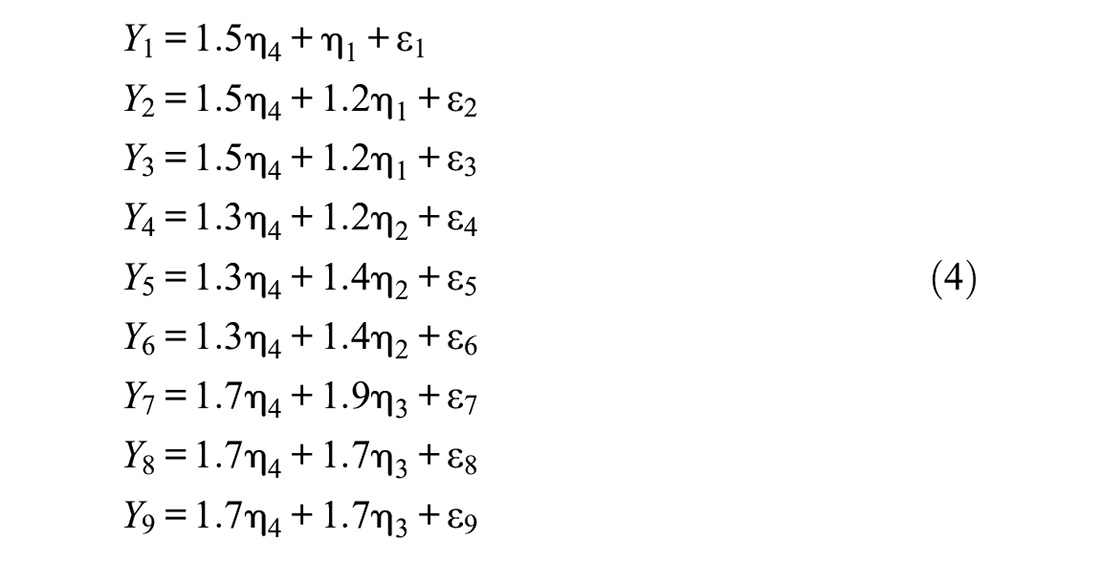
\begin{matrix} Y_{1} = 1.5 η_{4} + η_{1} + ε_{1} \\ Y_{2} = 1.5 η_{4} + 1.2 η_{1} + ε_{2} \\ Y_{3} = 1.5 η_{4} + 1.2 η_{1} + ε_{3} \\ Y_{4} = 1.3 η_{4} + 1.2 η_{2} + ε_{4} \\ Y_{5} = 1.3 η_{4} + 1.4 η_{2} + ε_{5} \\ Y_{6} = 1.3 η_{4} + 1.4 η_{2} + ε_{6} \\ Y_{7} = 1.7 η_{4} + 1.9 η_{3} + ε_{7} \\ Y_{8} = 1.7 η_{4} + 1.7 η_{3} + ε_{8} \\ Y_{9} = 1.7 η_{4} + 1.7 η_{3} + ε_{9} \end{matrix}

(4)

where the group factors η₁ through η₃ are independent standard normal variates, like the general factor η₄, and the residuals ε₁ through ε₉ are independent normal variates with variance 1.5 (cf. Muthén & Muthén, 2002, 2023). This data simulation process is implemented in the source code provided in Appendix 1 (and accomplished by its MODEL POPULATION command). (All results reported in the present section are replicated by employing that source code with the seed stated in it, at any of the above sample sizes, and then utilizing the source code in Appendix 2 for the following analyses with the respective set of 10,000 replications.)

We first observe that the nesting restrictions (3) do not hold in the (population) model generating the 30,000 data sets used in this section. Indeed, the ratio of general factor loading to respective first group factor loading changes from 1.25 to 1.5 when moving from either the third measure (Y₃) or the second measure (Y₂), to the first measure (Y₁). That is, this ratio is not constant within the set of three measures loading on the group factor η₁, but instead increases by a fourth of a latent standard deviation (of any of the four factors involved in the model) when moving from either Y₃ or Y₂ to Y₁, which is a considerable change. In addition, the ratio of the general factor loading of the fourth, fifth, or sixth measure to its respective second group factor loading, decreases by almost a sixth of a latent standard deviation when moving from the fourth to either the fifth or sixth measure, which is also a considerable drop. Moreover, the ratio of the general factor loading of the seventh, eighth, and nineth measure to its respective third group factor loading varies as well, in that it notably increases by more than a tenth of a latent standard deviation when moving from the seventh to either the eighth or nineth measure. Thus, in the data generation model, there are multiple and considerable violations of the restrictions (3) for all group factors, amounting (in a single violation) to up to a fourth of a latent standard deviation of the general and any group factors. Therefore, based on the earlier discussion in this section, one can conclude that the second-order factor model is not correct since its essential constraints (3) are markedly violated in multiple ways and locations within it. Thereby the extent of its misspecifications, considered in their totality, is marked rather than minimal—as reflected in the above explicated violations of the loading ratio constancy condition (3), with any single of them amounting up to a fourth of the variance of any factor involved in the data simulation model. Hence, the second-order factor model cannot be preferable to the bifactor model in the setting under consideration (which is the true model, having generated the 30,000 data sets analyzed in this section; see equations (4)).

With these observations in mind, we examine next the bifactor and second-order model fit results at each of the three sample sizes used, which are summarized in Table 1. (Fitting of the bifactor model is accomplished with the second part of the source code in Appendix 1, specifically by its MODEL section, and fitting of the second-order model is achieved with the source code in Appendix 2; see also Notes to both appendices.)

Table 1.

Goodness of Fit Indices for the Bifactor and Second-Order Models (Including BIC and Its Difference Between the Bifactor and Second-Order Models)

n:	700		1,000		2,000
n:	M_B(df = 18)	M_S(df = 24)	M_B(df = 18)	M_S(df = 24)	M_B(df = 18)	M_S(df = 24)
F *	.02598	.04595	.01817	.03545	.00903	.02316
LL *	−12,342.832	−12,349.809	−17,640.105	−17,648.736	−35.297.081	−35,311.204
χ ² *	18.163	32.117	18.152	35.414	18.055	46.302
BIC*	24,921.503	24,896.149	35,528.890	35,504.706	70,867.794	70,850.436
dBIC*	25.353		24.184		17.358

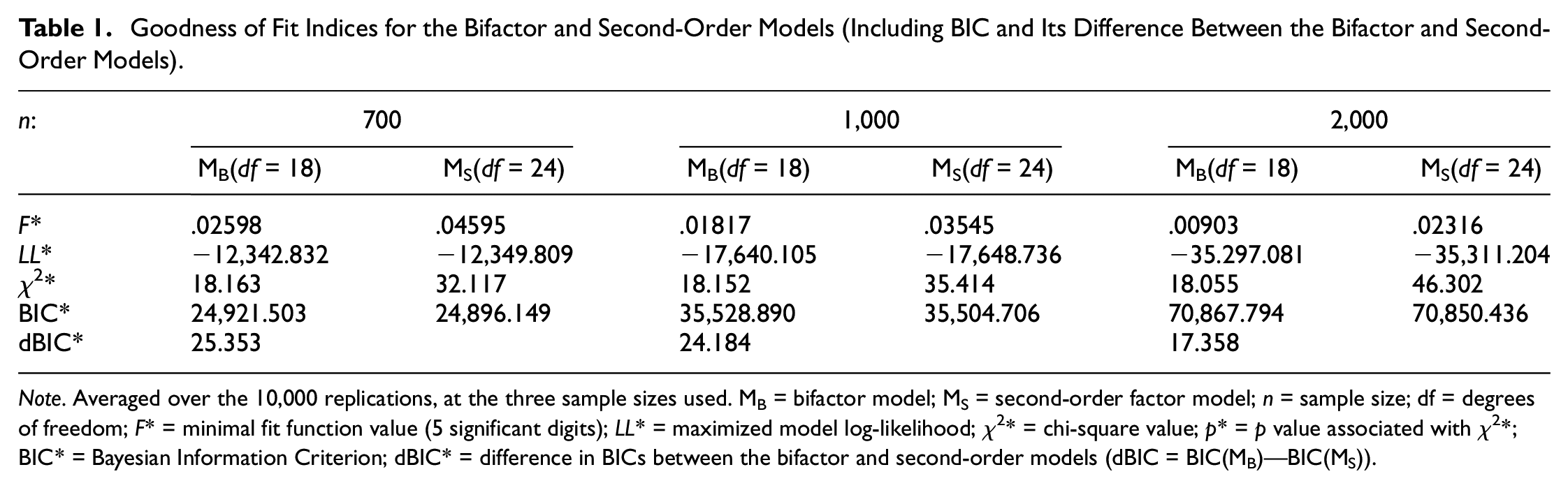
Note. Averaged over the 10,000 replications, at the three sample sizes used. M_B = bifactor model; M_S = second-order factor model; n = sample size; df = degrees of freedom; F* = minimal fit function value (5 significant digits); LL* = maximized model log-likelihood; χ²* = chi-square value; p* = p value associated with χ²*; BIC* = Bayesian Information Criterion; dBIC* = difference in BICs between the bifactor and second-order models (dBIC = BIC(M_B)—BIC(M_S)).

As seen from Table 1, the average minimized fit function value is larger for the second-order factor model, at each sample size, since this is a more restrictive model (being nested in the bifactor model, as pointed out earlier; e.g., Mansolf & Reise, 2017). Similarly, the maximized log-likelihood is on average lower for the second-order model at all sample sizes, again due to it being the more restricted model of the two considered. Correspondingly, the chi-square value is on average lower for the bifactor model for all sample sizes. Also these observations are consistent with the fact that the bifactor is the more relaxed of the two models, and all these model goodness of fit results are not unexpected, given the relationship between the second-order and bifactor models. As indicated earlier however, the focus of this note is not on any overall fit index but on the performance of the BIC as a model comparison index. Therefore, it is the BIC averages of the two models that are of focal interest here (see also discussion next and Table 2 below), which are found in the second-last row of Table 1. Upon inspection of these statistics, we notice that at each of the three sample sizes, the average BIC of the second-order model is smaller by more than 17 units relative to that of the bifactor model (see last row of Table 1). This indicates on average strong evidence in favor of preferring the considerably mis-specified, second-order model over the true, bifactor model that has actually generated all analyzed data sets (e.g., Raftery, 1995, p. 139).

Table 2.

Descriptive Statistics for the BIC Difference, dBIC, of the Bifactor, and Second-Order Models Over the 10,000 Replication Data Sets at the Three Sample Sizes Used (Stata Output Format; See Also Table 1)

n = 700:
	Percentiles:	Smallest:
1%	5.939453	−8.90625	Mean	25.35312
5%	13.17383	−8.462891	Std. dev.	6.641493
10%	16.39844	−8.160156	Variance	44.10942
25%	21.44531		Skewness	−.8101681
50%	26.23047		Kurtosis	3.860243
75%	30.28809	Largest:
90%	33.07715	38.41992
95%	34.41992	38.44141
99%	36.54688	38.55859
n = 1,000:
	Percentiles:	Smallest:
1%	2.832031	−21.36328	Mean	24.1845
5%	10.55078	−16.26563	Std. dev.	7.573627
10%	13.97266	−15.36719	Variance	57.35983
25%	19.74609		Skewness	−.755438
50%	25.10352		Kurtosis	3.891272
75%	29.71094	Largest:
90%	33.17383	39.73438
95%	34.8457	39.79688
99%	37.31836	40.02734
n = 2,000:
	Percentiles:	Smallest:
1%	−10.96094	−33.66406	Mean	17.35815
5%	−.6523438	−33.25000	Std. dev.	10.0854
10%	4.027344	−28.23438	Variance	101.7152
25%	11.29297		Skewness	−.6262846
50%	18.33203		Kurtosis	3.623781
75%	24.61328	Largest:
90%	29.47266	41.05469
95%	31.98047	41.14844
99%	36.125	41.91406

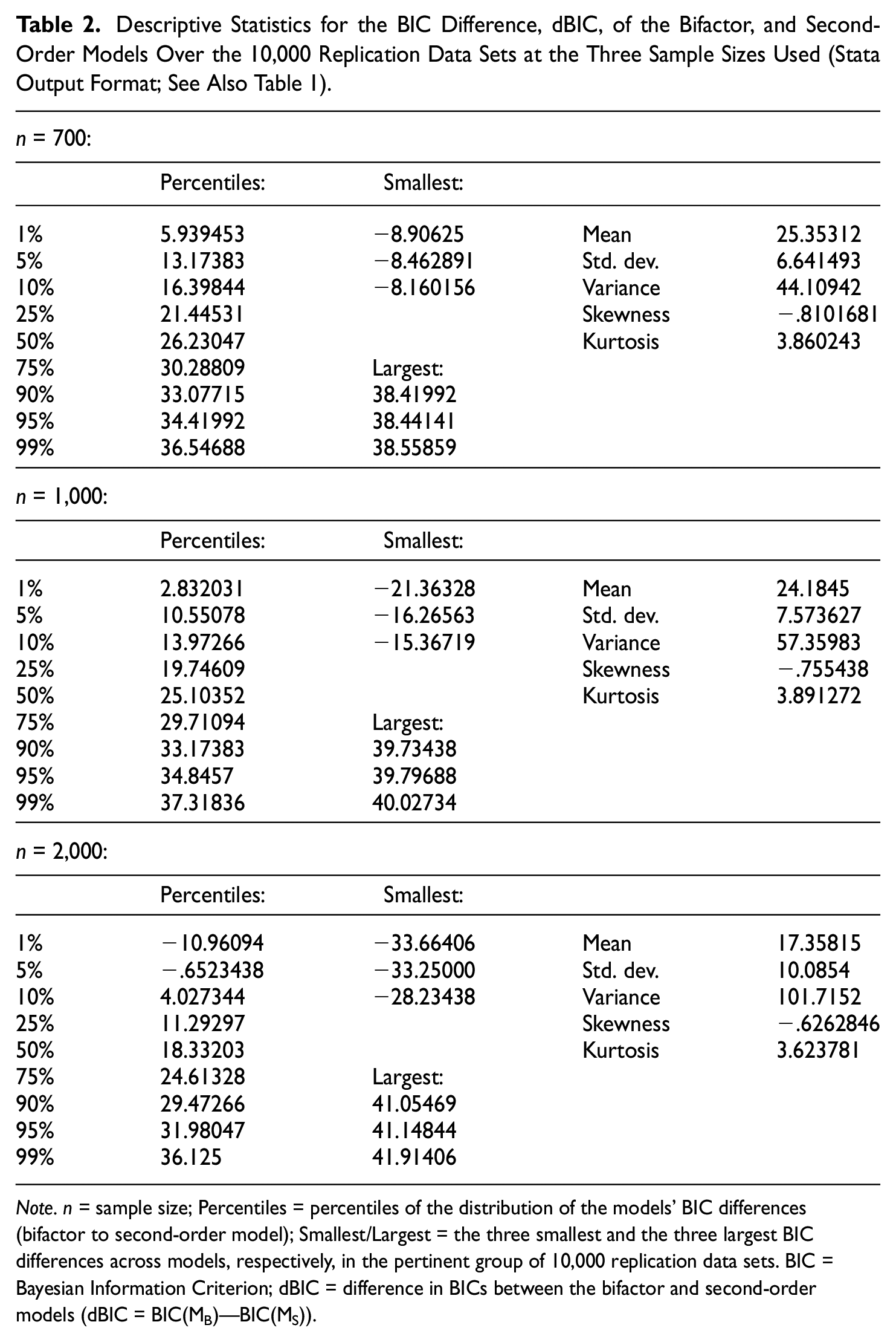
Note. n = sample size; Percentiles = percentiles of the distribution of the models’ BIC differences (bifactor to second-order model); Smallest/Largest = the three smallest and the three largest BIC differences across models, respectively, in the pertinent group of 10,000 replication data sets. BIC = Bayesian Information Criterion; dBIC = difference in BICs between the bifactor and second-order models (dBIC = BIC(M_B)—BIC(M_S)).

While Table 1 contains averages over the 10,000 replications for each sample size, Table 2 displays at them the descriptive statistics over these replications for the index of key relevance for this note, viz. the difference between the BICs of the bifactor and second-order factor models (in this order; see Table 1 for its pertinent averages). In addition, Figures 1 to 3 display the corresponding histograms of this difference at the three sample sizes.

Figure 1.

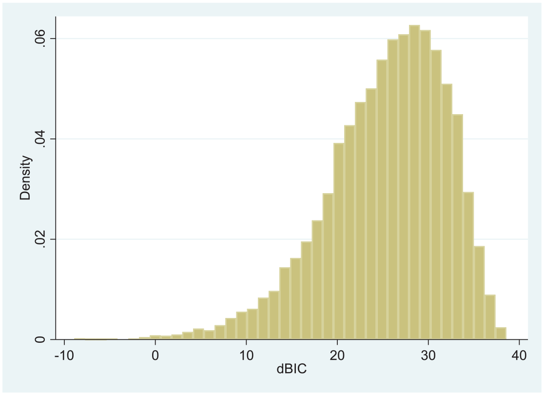
Histogram of the Difference, dBIC, of the BIC Indices for the Bifactor and Second-Order Factor Models at Sample Size 700

Figure 2.

Histogram of the Difference, dBIC, of the BIC Indices for the Bifactor and Second-Order Factor Models at Sample Size 1,000

Figure 3.

Histogram of the Difference, dBIC, of the BIC Indices for the Bifactor and Second-Order Factor Models at Sample Size 2,000

As seen from Table 2 as well as Figures 1 to 3, the overwhelming (if not vast) majority of the replication data sets at each sample size are associated with a smaller BIC for the second-order model, which is mis-specified, than the BIC for the bifactor model used to simulate all 30,000 data sets. At the same time, we also observe from both tables and these three figures that the degree to which the BIC of the second-order model is smaller than the BIC of the bifactor model, is slowly but noticeably decreasing as sample size grows. This seemingly weak trend is also apparent in Table 1, where the average of the pertinent BIC difference rather slightly decreases with increasing sample size. Similarly, the very limited area under the boundary (edge polygon) of the histogram of the BIC difference and to the left of 0 is also slowly increasing with sample size. These observations need not be unexpected and in fact may be seen as consistent with an apparent tendency of the BIC to prefer more complex models (like the bifactor model here) with larger samples (e.g., Bollen et al., 2014; Huang, 2017; see also Raykov & Zajacova, 2012, and next section).

With all above findings in mind, the results reported in this section show that the settings considered provide clear cases of the BIC being misleading when used for selecting between the bifactor and second-order factor models. The reason is that the latter is an incorrect model (due to (3) being violated in it), unlike the bifactor model that is the true model having generated the analyzed data. Hence, M_B would be expected to be found preferable to M_S at least in the majority of the 30,000 replications used if the BIC were to be generally dependable as an index for comparing these two models. This expectation is, however, clearly contradicted by the above findings showing that the BIC index in fact prefers the incorrect model M_S, at all sample sizes, rather than the correct model M_B in the overwhelming part if not nearly all of the 30,000 analyzed data sets (cf. Raftery, 1995). For this reason, we caution educational and behavioral scholars that the BIC may not be routinely relied on as a model selection index for the purpose of differentiating between the bifactor and second-order factor models in empirical research, especially at less than very large samples.⁴

Discussion and Conclusion

This note was concerned with the process of model comparison between the increasingly popular bifactor model in educational, psychological, and social research, and its widely used alternative, the second-order factor model that has potentially considerably distinct theoretical and empirical implications. The focus was on the query whether the popular BIC could be routinely depended on when a researcher is to choose between these two models in behavioral studies because they both are of high interest as means of description and explanation of data resulting from psychometric scales, tests, test batteries, or sets of used manifest measures. The preceding discussion questioned routine reliance on the BIC as an index for selecting between the bifactor and second-order models. This argument was based on empirically widely applicable settings of multiple measuring instrument components used to generate at different sample sizes a very large number of data sets following the bifactor model with markedly violated, essential restrictions characterizing the second-order model. On these data, however, the BIC consistently preferred the incorrect second-order model rather than the correct bifactor model, thus failing a scholar using it as a comparison index for the models. With these findings, the present article extends earlier simulation-based research on the bifactor model in relation to other rival models (e.g., Bader & Moshagen, 2022; Gignac, 2016; Greene et al., 2019; Molenaar, 2016; Murray & Johnson, 2013). In particular, we add to that prior research readily repeatable and transparent results that do not support a possible general claim of overall goodness of fit bias in favor of the bifactor model. Specifically, such a bias is not generally the case with respect to the BIC index for samples that are not very large.

Several potential generalizations of the findings of the present note need to be rejected at this point because they are not made or attempted in it. First of all, the note does not intend to imply, nor does it imply, that one should question the general utility of the BIC as a model comparison index in educational and psychological studies and well beyond them. This is because the article provides only specific and limited evidence, which thus cannot be used to make a more general statement that was therefore not alluded to, indicated, or advanced in it. Second, the note does not imply or suggest that the BIC will frequently fail when used for selecting between the bifactor and second-order models, or in other empirical studies. At the same time, it is worth pointing out that we are not aware of instructive discussions in the extant literature that could shed light on how frequently and when specifically findings of BIC failure of the type discussed may occur in empirical research. Hence, the question of how often and when the BIC could fail scholars involved in these models’ comparison, remains open. Third, and relatedly, the note does not imply or suggest in any way that the failure of the BIC demonstrated in its last section is to be expected to persist at any sample size. In fact, based on the presented findings, it appears that this behavior of BIC may not necessarily be frequently observed at (considerably) larger sample sizes than those used. How large these sample sizes could be, is likely to depend on the particulars of the used models, including probably number of observed and latent variables, reliability of individual measures, and more generally fraction of missing values (see, e.g., Huang, 2017, for the BIC’s asymptotic behavior consistent with selecting more complex models with lower population minimal discrepancy values). Fourth, we do not imply that the BIC is the only possible model comparison means that could or should be used for selecting between the bifactor and second-order models. For example, likelihood ratio tests (LRTs; e.g., under normality) or corrected LRTs (with some violations of normality) can in addition be used to examine the validity of the nesting restrictions in equations (3), and depending on their results selection from these two models can then be carried out (e.g., Mansolf & Reise, 2017; Yung et al., 1999; see also Satorra & Bentler, 2001). Furthermore, the Akaike Information Criterion (AIC) need not share the same downside of the BIC exemplified in this note, at least not to the same extent (see also Footnote 3), and hence provides a useful complement to other model comparison procedures. Similarly, and especially with large samples when the LRT power may be excessive, the approach of effect size evaluation for nested models outlined by Raykov, DiStefano, Calvocoressi, & Volker (2022) can also be used as a complement to these procedures for model choice.^5,6 Last but not least, given the results of this note, we encourage future and extensive stimulation studies on BIC’s performance that vary not only (a) sample size (as in this article), but also (b) number of observed variables, (c) number of group factors in the bifactor model (and thus of first-order factors in the second-order model), and (d) the extent of violation of the nesting restrictions (3), in particular including varying degrees of discrepancies in the ratios of general to group factor loadings. These studies go well beyond the confines of the present article whose aim was solely to caution empirical scholars against routine reliance on the BIC as a model comparison index, especially at sample sizes that are not very large, when studying the bifactor and second-order factor models.⁷ With this in mind, the findings of the article cannot substantiate a more general criticism of the BIC beyond the limited scope of the empirical settings considered and with samples that are not impressively large. Therefore, such a criticism was not intended, raised, or implied in this note. For this reason, its results merely complement the voluminous body of literature on model comparison and in particular on the BIC features, without overriding or questioning any general findings of prior research on model comparison and the BIC’s utility in it.

In conclusion, this note was concerned with two theoretically and empirically important means for description and explanation of data resulting from psychometric scales, tests, or multicomponent measuring instruments widely used in educational and psychological research, the bifactor and the second-order factor models. The note raised caution that the popular BIC may not routinely be viewed as a dependable model comparison index, especially with less than very large samples, by scholars interested in selecting between these two increasingly popular models in empirical studies.

Footnotes

Appendix

Appendix 2

Mplus Source Code for Fitting the Second-Order Factor Model to the 10,000 Replication Data Sets

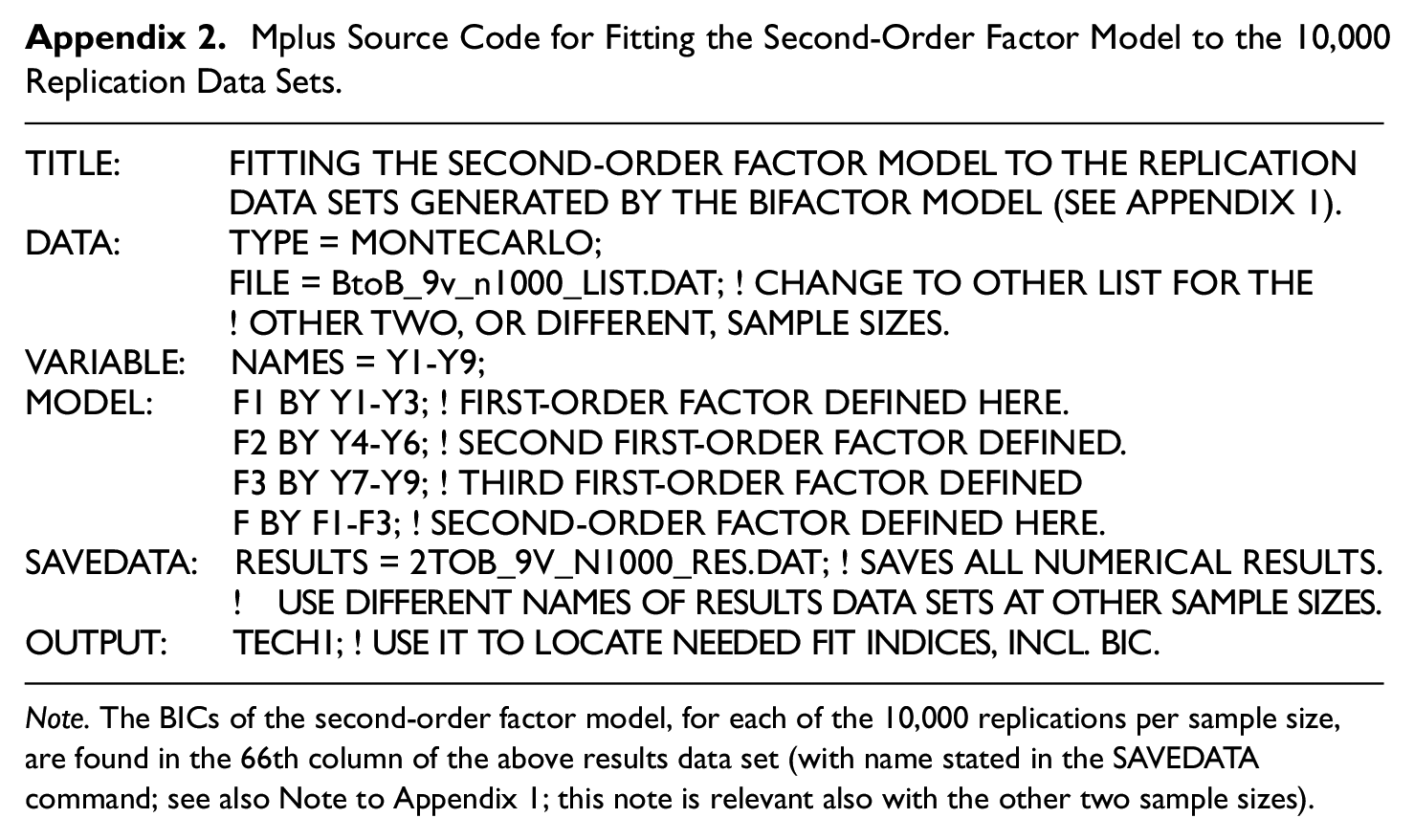
TITLE: FITTING THE SECOND-ORDER FACTOR MODEL TO THE REPLICATION
DATA SETS GENERATED BY THE BIFACTOR MODEL (SEE APPENDIX 1).
DATA: TYPE = MONTECARLO;
FILE = BtoB_9v_n1000_LIST.DAT; ! CHANGE TO OTHER LIST FOR THE
! OTHER TWO, OR DIFFERENT, SAMPLE SIZES.
VARIABLE: NAMES = Y1-Y9;
MODEL: F1 BY Y1-Y3; ! FIRST-ORDER FACTOR DEFINED HERE.
F2 BY Y4-Y6; ! SECOND FIRST-ORDER FACTOR DEFINED.
F3 BY Y7-Y9; ! THIRD FIRST-ORDER FACTOR DEFINED
F BY F1-F3; ! SECOND-ORDER FACTOR DEFINED HERE.
SAVEDATA: RESULTS = 2TOB_9V_N1000_RES.DAT; ! SAVES ALL NUMERICAL RESULTS.
! USE DIFFERENT NAMES OF RESULTS DATA SETS AT OTHER SAMPLE SIZES.
OUTPUT: TECH1; ! USE IT TO LOCATE NEEDED FIT INDICES, INCL. BIC.

Note. The BICs of the second-order factor model, for each of the 10,000 replications per sample size, are found in the 66th column of the above results data set (with name stated in the SAVEDATA command; see also Note to Appendix 1; this note is relevant also with the other two sample sizes).

Acknowledgements

The authors thank T. Asparouhov for valuable discussions on factor model simulation software, as well as to the Editor and three anonymous Referees for critical comments on an earlier version of the paper that have contributed considerably to its improvement.

Declaration of Conflicting Interests

The author(s) declared no potential conflicts of interest with respect to the research, authorship, and/or publication of this article.

Funding

The author(s) received no financial support for the research, authorship, and/or publication of this article.

ORCID iDs

Tenko Raykov

Christine DiStefano

Notes

References

Bader

Moshagen

(2022). Assessing the fitting propensity of factor models. Psychological Methods. Advance online publication. https://doi.org/10.1037/met0000529

Bentler

P. M.

Chou

C.-P.

(1987). Practical issues in structural equation modeling. Sociological Methods and Research, 16, 78–117.

Bollen

K. A.

(1989). Structural equations with latent variables. Wiley.

Bollen

K. A.

Harden

J. J.

Ray

Zavisca

(2014). BIC and alternative Bayesian information criteria in the selection of structural equation models. Structural Equation Modeling, 21, 1–19.

Cudeck

MacCallum

R. C.

(2007). Factor analysis at 100. Lawrence Erlbaum Associates.

Gignac

G. E.

(2016). The higher-order model imposes a proportionality constraint: That is why the bifactor model tends to fit better. Intelligence, 55, 57–68.

Greene

A. L.

Eaton

N. R.

Forbes

M. K.

Krueger

R. F.

Markon

K. E.

Waldman

I. D.

Cicero

D. C.

Conway

C. C.

Docherty

A. R.

Fried

E. I.

Ivanova

M. Y.

Jonas

K. G.

Latzman

R. D.

Patrick

C. J.

Reininghaus

Tackett

J. L.

Wright

A. G. C.

Kotov

(2019). Are fit indices used to test psychopathology structure biased? A simulation study. Journal of Abnormal Psychology, 128, 740–764.

Huang

P.-H.

(2017). Asymptotics of AIC, BIC, and RMSEA for model selection in structural equation modeling. Psychometrika, 82, 407–426.

Jennrich

R. I.

Bentler

P. M.

(2011). Exploratory bi-factor analysis. Psychometrika, 76, 537–549.

10.

Jennrich

R. I.

Bentler

P. M.

(2012). Exploratory bi-factor analysis: The oblique case. Psychometrika, 77, 442–454.

11.

Mansolf

Reise

S. P.

(2017). When and why the second-order and bifactor models are distinguishable. Intelligence, 61, 120–129.

12.

Markon

K. E.

(2019). Bifactor and hierarchical models: Specification, inference, and interpretation. Annual Review of Clinical Psychology, 15, 51–69.

13.

Molenaar

(2016). On the distortion of model fit in comparing the bifactor model and the higher-order factor model. Intelligence, 57, 60–63.

14.

Mulaik

S. A.

(2009). Foundations of factor analysis. CRC Press.

15.

Murray

A. L.

Johnson

(2013). The limitations of model fit in comparing the bi-factor versus higher-order models of human cognitive ability structure. Intelligence, 41, 407–422.

16.

Muthén

L. K.

Muthén

B. O.

(2002). How to use a Monte Carlo study to decide on sample size and determine power. Structural Equation Modeling, 9, 599–620.

17.

Muthén

L. K.

Muthén

B. O.

(2023). Mplus user’s guide. Muthén & Muthén.

18.

Rabe-Hesketh

Skrondal

(2022). Multilevel and longitudinal modeling with Stata (4th ed.). Stata Press.

19.

Raftery

A. E.

(1995). Bayesian model selection in social research. Sociological Methodology, 25, 111–163.

20.

Raykov

DiStefano

(2021). Evaluating restrictive models in behavioral research: Local misfit overrides overall model plausibility. Educational and Psychological Measurement, 81, 980–995.

21.

Raykov

DiStefano

Calvocoressi

Volker

(2022). On effect size measures for nested measurement models. Educational and Psychological Measurement, 82, 1225–1246.

22.

Raykov

Marcoulides

G. A.

(2006). A first course in structural equation modeling. Lawrence Erlbaum Associates.

23.

Raykov

Marcoulides

G. A.

Chang

(2016). Studying population heterogeneity in finite mixture settings using latent variable modeling. Structural Equation Modeling, 23, 726–730.

24.

Raykov

Zajacova

(2012). On latent change model choice in longitudinal studies. Structural Equation Modeling, 19, 580–592.

25.

Reise

S. P.

(2012). The rediscovery of bifactor measurement models. Multivariate Behavioral Research, 47, 667–696.

26.

Reise

S. P.

Mansolf

Haviland

M. G.

(2023). Bifactor measurement models. In Hoyle

(Ed.), Handbook of structural equation modeling (2nd ed., pp. 329–348). Guilford Press.

27.

Rindskopf

(1984). Structural equation models: Empirical identification, Heywood cases, and related problems. Sociological Methods & Research, 13, 109–119.

28.

Satorra

Bentler

P. M.

(2001). A scale difference chi-square test statistic for moment structure analysis. Psychometrika, 66, 507–514.

29.

Yang

Spirtes

Scheines

Reise

S. P.

Mansolf

(2017). Finding pure submodels for improved differentiation of bifactor and second-order models. Structural Equation Modeling, 24, 402–413.

30.

Yung

Y.-F.

Thissen

McLeod

L. D.

(1999). On the relationship between the higher-order factor model and the hierarchical factor model. Psychometrika, 64, 113–128.