Structural Covariates of Gang Homicide in Large U.S. Cities

Abstract

Objectives:

This study examined the structural covariates of gang homicide in large U.S. cities and whether the structural conditions associated with gang homicide differed from non-gang homicide.

Methods:

Several national data sources were used to gather information on the structural conditions of the 88 largest U.S. cities, including the U.S. Census Bureau, Law Enforcement Management and Administrative Statistics, Uniform Crime Report, and National Gang Center. Negative binomial regression was used to model the relationship between the structural conditions of cities and homicide rates.

Results:

Socioeconomic deprivation, official rates of gang membership, and population density explained between-city variability in gang homicide rates. In addition, quadratic associations were observed for socioeconomic deprivation and population density. Equality of coefficients tests revealed that the structural covariates of gang homicide differed in magnitude from non-gang homicide.

Conclusions:

Prior to this study, the etiology of gang homicide was found to differ from other homicide types in terms of event characteristics and sub-city correlates. This macro-level study extended this line of research to cities, providing evidence that the structural correlates of violence operated differently for gang homicide.

Keywords

gangs homicide structural covariates

Homicide has been the subject of social science research for decades (Baller et al. 2001; Henry and Short 1954; Land, McCall, and Cohen 1990; Wolfgang 1958). A particularly influential line of research has focused on the structural correlates of homicide. Factors linked to resource deprivation and population structure have been found to account for a large proportion of variation in homicide rates in neighborhoods, cities, and counties (Land et al. 1990; McCall, Land, and Parker 2010; Smith and Zahn 1999). Over the past two decades, a major theme in homicide research has been to disaggregate—by participant demographics or by homicide types—to determine the empirical efficacy of established covariates (Flewelling and Williams 1999; Krivo and Peterson 2000; Kubrin 2003; Parker 2004). Invariances observed across units of analysis and disaggregated categories increase the theoretical and empirical adequacy of structural correlates, thus leading to better specified models and a more comprehensive understanding of the underlying sources of homicide.

A serious void in this line of research is the shortage of attention directed toward gang homicide. Gangs account for a sizable share of homicide totals across various levels of analysis—neighborhoods, cities, counties, and states—typically between 10 and 50 percent (Braga et al. 2003; Decker and Pyrooz 2010a; Maxson, Gordon, and Klein 1985; Tita and Abrahamse 2004). At this point in time, however, criminological knowledge about gang homicide is limited to analyses of event characteristics and sub-city correlates. Homicide event research indicates that gang homicides differ from non-gang homicides in terms of settings and participants (Maxson et al. 1985), thus requiring specialized attention from police and prosecutors (Katz and Webb 2006; Pyrooz, Wolfe, and Spohn 2011). Studies examining the neighborhood correlates of homicide have demonstrated that gang homicides differ from non-gang homicides in Chicago and St. Louis neighborhoods (Kubrin and Wadsworth 2003; Mares 2010; Papachristos and Kirk 2006; Rosenfeld, Bray, and Egley 1999); however, inconsistent findings prevent the establishment of a general knowledge base.

An overarching problem is the absence of macro-level gang homicide research. Given the prevalence of gang homicide—especially in large U.S. cities—this poses a host of problems for gang and homicide researchers alike. For gang researchers, this void prevents researchers from knowing if city-specific findings are simply city-specific. The most serious drawback is that criminologists can only speculate when asked why City A has a higher rate of gang homicide than City B. For homicide researchers, “gang” is among the only major category of homicide unexamined at the city level. The extent to which the structural conditions underlying gang homicide are consistent with the larger body of research is unknown.

This study addresses these shortcomings by advancing a macro-level analysis of gang homicide in large U.S. cities. Herein, I seek to accomplish two goals: (a) identify structural covariates of gang homicide, which will extend the understanding of gang homicide from a localized (i.e., within-city) to a generalized (i.e., between-city) state of knowledge, thus providing an explanation to why some cities have higher rates of gang homicide than others and (b) examine whether structural covariates of gang homicide differ from that of non-gang homicide, which will determine the extent to which the conditions associated with gang homicide are consistent with aggregate and disaggregated homicide studies.

Homicide and Disaggregation

The United States has averaged around 15,000–17,000 homicides over the last decade (FBI 2010). Explaining the variation of homicide across various units of aggregation has been a staple in social science research (Daly and Wilson 1988; Land et al. 1990; Smith and Zahn 1999). Until 1990, structural covariates linked to demographic (e.g., percent black and racial/ethnic heterogeneity), social (e.g., percent divorced and single-parent households), economic (e.g., poverty, income inequality, and unemployment), and population (e.g., density and size) factors were found to vary inconsistently across research contexts. Given that homicide is a (if not the) key indicator of violence, inconsistent findings invoked confusion into the status of structural theories. In what is perhaps the most influential study on homicide, Land et al. (1990) examined rates of homicide in cities, metropolitan areas, and states across four successive decades, finding that resource deprivation, population structure, and divorce rates reliably explained homicide rates, regardless of the unit of analysis or time period parameters (see also McCall et al. 2010).

Since Land et al.’s (1990) study ironed out the inconsistencies surrounding structural covariates of homicide, the homicide literature has proceeded in two ways. First, researchers have focused on refining the literature by way of testing reconceptualized and operationalized covariates or established findings with contemporary methods (Avakame 1997; Baller et al. 2001; Cohen and Tita 1999; Kubrin and Herting 2003; Kovandzic, Vieraitis, and Yeisley 1998; McCall et al. 2010; Wadsworth and Kubrin 2004). Second, researchers have focused on disaggregating homicide by participant demographics or by homicide types to determine the robustness of theoretical explanations (Flewelling and Williams 1999; Kubrin 2003; Parker 2004; Pizarro 2008; Steffensmeier and Haynie 2000). Both routes have extended the understanding of homicide considerably, but disaggregation has been especially useful because of the empirical challenge it poses by modeling relationships under different specifications.

Williams and Flewelling (1988) were among the first to suggest that the dependent variable should be disaggregated in homicide studies. They held that researchers tend to “analyze the homicide rate as if it were a homogeneous category of lethal violence” (Williams and Flewelling 1988:422) when instead homicides should be parceled into categories. The disaggregation route would result in a better explanation because the “total rate of homicide is a useful indicator for the overall levels of lethal interpersonal violence, just as the Dow Jones Industrial Average provides an overall gauge of the strength of securities in the United States” (Flewelling and Williams 1999:99). In other words, much like how the performance of different market sectors is better explained by factors unique to the sector rather than factors general to the market, “sectors” of homicide should be better explained by specific rather than general structural conditions as well.

Kubrin and Wadsworth (2003) carried out an analysis along these lines by examining African American homicides in St. Louis neighborhoods. Their measure of disadvantage, a common predictor in most homicide studies, was associated with aggregate homicide. When the data were disaggregated by homicide type, however, the effect of disadvantage mattered for gang, intimate, stranger, and nonstranger homicide but did not for stranger and nonstranger robbery homicides. The masking of the robbery effects contains both policy and theoretical relevance. Practically, it demonstrates that situational crime prevention efforts are limited insofar as they are based on place-based factors such as disadvantage. Conceptually, the implication from this line of research is that if invariance is not observed across homicide types, it calls into question the generality of correlates. In other words, it may be necessary to rethink theory arguing that disadvantage is an underlying source of robbery homicide in neighborhoods. Researchers have focused carefully on various homicide types, such as drug, robbery, intimate partner, hate, law enforcement, multiple or mass, and—the focus of the present study—gang homicide.

There are key differences between gang and other types of homicide. A large body of research has examined these differences in gang homicide incidents, in terms of participants and settings. Maxson et al. (1985) made this comparison using data gathered from the Los Angeles police and sheriff’s departments between 1978 and 1982. They found that gang homicide events, compared to non-gang homicide events, involved younger suspects and victims, multiple suspects, strangers, minorities, and occurred in public settings. These findings have been replicated almost uniformly, with supporting evidence in cities such as Chicago (Block and Block 2005 [as cited in Mares 2010]; Curry and Spergel 1988), Los Angeles (Hutson et al. 1995), Newark (Pizarro and McGloin 2006), and St. Louis (Decker and Curry 2002; Kubrin and Wadsworth 2003), and research carried out on states such as California (Bailey and Unnithan 1994; Tita and Abrahamse 2004).

The invariance of gang homicide event differences across study sites, time periods, and units of analysis has led scholars to conclude that gang homicides are distinct from other types of homicide (Howell 1999; Maxson 1999; Maxson, Curry, and Howell 2002). Qualitative and quantitative research supports this argument, finding unique features of gang violence such as drive-by and walk-up shootings and epidemic and retaliatory processes consistent with spatial dependence themes (Cohen and Tita 1999; Decker 1996; Miller and Decker 2001; Papachristos 2009; Rosenfeld et al. 1999; Sanders 1994). This raises the question that if there are empirical differences at the event level and differences in the nature and processes of gang violence, there may also be differences in the structural conditions associated with gang homicide.

Covariates of Gang Homicide

A number of studies have attempted to explain the nonrandom geographical distribution of gang homicides within cities. Most of this research has been carried out in a handful of cities, including Chicago (Curry and Spergel 1988; Mares 2010; Papachristos and Kirk 2006), Los Angeles (Kyriacou et al. 1999), and St. Louis (Kubrin and Wadsworth 2003; Rosenfeld et al. 1999). These studies all varied in their conceptual and analytic focus, with some seeking to identify gang homicide predictors and others seeking to test theory. In particular, four of the studies—Kubrin and Wadsorth (2003), Mares (2010), Papachristos and Kirk (2006), and Rosenfeld et al. (1999)—shed light on the conceptual argument to disaggregate, finding evidence to support this argument (but see Rosenfeld et al.1999:513-14).¹ For example, based on 800 census tracts in Chicago, Mares (2010) found that the effect of all three social disorganization covariates—disadvantage, residential instability, and population heterogeneity—differed for gang homicide in relation to drug, intimate, and robbery non-gang homicides. When Mares compared gang to aggregate non-gang homicide types, disadvantage and residential instability differed statistically, leading him to conclude that the structural factors underlying gang homicide differed from other types of homicide.

There is conflicting evidence, however, whether there is a set of consistent predictors of gang homicide. Of the studies mentioned above, only variants of socioeconomic deprivation exhibited consistency in statistical significance. Divergent effects could be conceivable between cities, although unfavorable theoretically, but this has been observed even within the same city of analysis. For example, Kubrin and Wadsworth (2003) and Rosenfeld et al. (1999) both examined correlates of gang-motivated homicide in St. Louis between 1985 and 1995. While the unit of analysis differed (census tracts vs. blocks), there was variance in statistical significance between the studies for disadvantage, instability, population size, and spatial lag effects.²

There are at least four factors that could be responsible for the inconsistency in correlates of gang homicide between and within cities. First, divergences between cities could be due to different mechanisms in place influencing gang homicide rates. Second, this discrepancy may be due to model specification and intervening variables. For example, Papachristos and Kirk (2006) incorporated collective efficacy into their analysis of gang homicide in Chicago neighborhoods, finding that it partially mediated the influence of structural factors such as concentrated disadvantage. Third, as Land et al. (1990) observed in their study, the partialling fallacy may have introduced problems in studies not employing principle components approaches to account for shared variance. Finally, as Hipp (2007) demonstrated, some factors operate differently across levels of aggregation, which is the likely explanation for the inconsistency between Rosenfeld et al. and Kubrin and Wadsworth’s findings.

In summary, readers are left with an incomplete story for understanding the structural conditions associated with gang homicide. A notable void in this line of research is the lack of macro-level analysis. That is, most gang homicide research has been carried out within cities instead of between cities. While there is both conceptual and empirical support to disaggregate gang homicide, this support has been found only at the incident and neighborhood level. Given the moderate prevalence of gang homicide in cities' overall homicide tallies and the inconsistencies identified above in the extant literature, a macro-level analysis is needed to extend the state of knowledge in the gang and homicide literatures.

Current Study

This study analyzes gang homicide in large U.S. cities. This research has two goals: (a) identify structural covariates of gang homicide and (b) examine whether structural covariates of gang homicide differ from non-gang homicide. Related to the first goal, Howell (1998:9) asserted that “[l]evels of gang violence differ from one city to another,” but at this point in time the literature offers no explanation backed by empirical evidence as to why. Related to the second goal, homicide researchers are missing a key piece of the disaggregation puzzle in examining the structural correlates of homicide. That is to say, scholarship at the incident and neighborhood level provides evidence that there are substantive differences in the underlying sources of gang and non-gang homicides, but this has yet to be extended to the city level. This study seeks to redress these issues.

Method

Data

The data for the present study were drawn from four national sources: the U.S. Census Bureau (2000), the Law Enforcement Management and Administrative Statistics survey or LEMAS (United States Department of Justice, Bureau of Justice Statistics 2000), the Uniform Crime Report (2002–2006), and the National Gang Center (2002–2006).³ U.S. Census data were used for information about social, economic, and population characteristics of cities, LEMAS data provided information with respect to law enforcement agency characteristics, Uniform Crime Report data were used to obtain information about homicide in cities, and National Gang Center data supplied information on gang membership and gang homicide in cities. Based on the 2000 census, the 88 most populated cities in the United States are included in the sample, with the least populated city containing about 200,000 residents.⁴ Large cities were the focus of the present examination to ensure substantial variation in the dependent variable. While gang activity is observed in rural and suburban areas, serious problems such as violence are more common in large cities (Maxson 1999; Maxson et al. 2002). To establish causal sequencing, the year 2000 was used as a benchmark for the explanatory variables and the outcome was measured thereafter.

Dependent Variables

Gang homicide is the key dependent variable for this study. This measure was drawn from the National Gang Center’s survey of law enforcement agencies between 2002 and 2006.⁵ A 5-year average of gang homicide incidents in cities was computed to account for year-to-year fluctuations. Using contemporaneous U.S. Census population estimates for the cities, averages were transformed into homicide rates per 100,000 citizens. Measures of non-gang homicide and total homicide, drawn from the Uniform Crime Report, were computed in a similar manner using U.S. Census population estimates and rate transformation.⁶ Some cities did not report homicide tallies for all of the study years. In these cases, the average was computed as long as values were present for at least two periods.

Law enforcement gang data have been found to be a useful indicator of gang activity in cities (Decker and Pyrooz 2010b; Katz and Schnebly 2010; Katz, Ballance, and Britt 2005; Katz, Webb, and Schaefer 2000; Maxson 1999; Pyrooz, Fox, and Decker 2010). Decker and Pyrooz (2010b) recently assessed the reliability and validity of gang homicide data in large U.S. cities from the National Gang Center (NGC) and Supplemental Homicide Report (SHR). They found that both reporting systems exhibited strong internal reliability over a 5-year period. In addition, the data were consistent with the principles of the convergent-discriminant validity test and demonstrated external validity. But the results of their supplementary analysis revealed that the NGC data outperformed the SHR data, as the reliability of the latter was conditioned by the presence of a specialized gang unit. For this reason, Decker and Pyrooz (2010a:371) recommended that “researchers avoid the general measurement system (SHR) in favor the specialized system (NGC), as it will provide a more accurate picture of gang homicide in cities.” This suggests that using NGC data for the dependent variable is appropriate in this study, as it has satisfied important measurement tests.⁷

It is important to note that gang member-based homicides were used as the outcome, as opposed to gang motive-based homicides. A homicide is considered member based if it involves a gang member as an offender or a victim.⁸ For homicides to be considered gang motivated, incidents must include furthering the objectives of the gang as a motive (e.g., protecting turf or attacking rivals). Maxson and colleagues (1985; Maxson and Klein 1990, 1996) have demonstrated that with the exception of the raw totals, there are few differences between member- and motive-based gang homicides; however, the former casts a wider net. The gang homicide literature has employed both definitions with equal fidelity. It was elected to proceed with the more inclusive member-based definition because motive-based homicides are ultimately a subset of member-based homicides and there is the potential to lose out on a wealth of valuable information by constraining the outcome to motive-based homicides exclusively (see Maxson and Klein 1990; Papachristos 2009:86).

Independent Variables

Drawing from the homicide and gang literatures, seven theoretical measures and statistical controls are used in the analyses.

First, a key explanatory variable in this study is gang membership rates. Structural factors should lead to varying levels of gang membership in cities (e.g., Pyrooz et al. 2010). Thus, gang membership should perform empirically as an intervening variable, mediating the influence of structural factors on gang homicide rates.⁹ Gang membership rates was operationalized using National Gang Center data on the number of gang members reported by the police (see National Youth Gang Center 2009). This measure was computed by taking a multiyear average (2002–2006) that was converted into a rate per 10,000 citizens based on contemporaneous U.S. Census population estimates.¹⁰ While this measure is an estimate and could be subject to measurement error, previous studies have used similar measures effectively (see Katz et al. 2000; Katz et al. 2005; Pyrooz et al. 2010). Further, strong internal reliability (mean inter-item r = .92) in combination with taking the multiyear average helps reduce concern for measurement error.

Next, deriving from various theories of crime and violence (e.g., anomie theory and social disorganization theory), socioeconomic deprivation and population heterogeneity were included as structural covariates. Socioeconomic deprivation is hypothesized as the backbone to many classic and contemporary criminological theories and has been found to be among the strongest predictors of homicide rates. In Land et al.’s study, resource deprivation exerted an effect size of over .50 across four successive decades of homicide. A key finding in Land et al.’s study was that while there may be conceptual differences in items such as relative deprivation/inequality, absolute deprivation, and African American population composition, these items were not “distinct empirically” (1990:944). Similarly, population heterogeneity holds central positions in theories emphasizing that increased social distance serves as an antecedent to reduced social cohesion and collective norms.

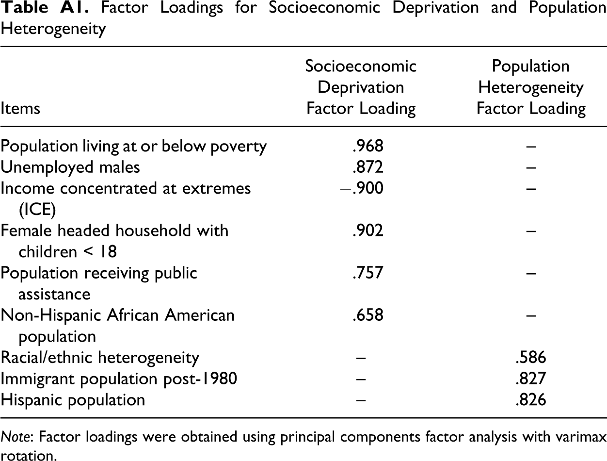
Similar to Land et al. and more recent homicide research (e.g., McCall et al. 2010; Parker, McCall, and Land 1999), principal components factor analysis was used to identify the underlying dimensions of socioeconomic deprivation and population heterogeneity. Items typically associated with socioeconomic deprivation and population heterogeneity—absolute deprivation (population living in poverty), inequality or relative deprivation (concentration at the extremes: Morenoff, Sampson, and Raudenbush 2001), African American population, female-headed households with children under 18 years of age, population receiving public assistance, male unemployment, racial/ethnic heterogeneity (Herfindahl index: Gibbs and Martin 1962; Blau 1977),¹¹ Hispanic population, and immigrant population post-1980—were entered into a principal axis factoring model using varimax rotation. Two factors emerged using .50 cut-off points for the factor loadings (Appendix A), accounting for 73 percent of the variance and eigenvalues of 4.37 and 2.15. Higher scores on these measures indicate greater deprivation and heterogeneity.

Four additional theoretical and statistical controls were included in the analytic models. Derived from social disorganization theory, residential stability was measured by identifying the percentage of the population inhabiting the same residence since 1995. Population density, the natural log of persons per square mile, is typically conceptualized as having theoretical linkages to urbanism (Wirth 1938) or routine activities/opportunity (Cohen and Felson 1979) theories. Population density is conceptualized as being consistent with the latter for gang homicide because threat and retaliation (Decker 1996; Papachristos 2009) should be amplified in close quarters. Next, youth population, measured as the percentage of the population between ages 10 and 24, taps into the age structure of cities. The relationship between age, crime, and gang activity is well documented in the literature (Hirschi and Gottfredson 1983; Huff 1998; Klein and Maxson 2006). Finally, gang unit is included as a statistical control for whether police departments maintained a specialized gang unit.¹²

Analytic Strategy

The analysis that follows begins by discussing the descriptive characteristics of cities and the bivariate associations between the study variables. Next, a series of multivariate negative binomial regression models are estimated to identify structural covariates of gang homicide in cities. The most fully specified gang homicide model is then applied to non-gang and total homicides, using tests to assess coefficient differences. All of the explanatory variables were standardized to evaluate effect sizes. The analyses were carried out in STATA 10.0 using heteroscedasticity-consistent robust standard errors (i.e., Huber-White standard errors). City population was used as an exposure variable permitting the findings to be interpreted as variations in homicide rates (Osgood 2000).¹³

Results

Summary Statistics

Table 1 displays the means, standard deviations, and ranges for the study variables. There were nearly 12 homicides per 100,000 citizens among the sample cities, which is about twice as great as the average homicide rate for the United States. There were two gang homicides per 100,000 citizens, accounting for 17 percent of the average homicide rate. The prevalence of gang homicide increases, however, when the denominator shifts to incidence, where over 20 percent of homicides in large cities were reportedly gang related. Gang homicide rates vary from 0 to 10 among the sample cities, although the majority reported a gang homicide rate below 4. The mean rate of gang membership was nearly 52 per 10,000 citizens, translating into a prevalence of less than 1 percent of the population. These figures take on added significance when considering that they are oriented mostly around males, adolescents and young adults, and minorities in urban areas (National Youth Gang Center 2009)—populations that are at a high risk for violent victimization. These summary statistics indicate that gang homicides comprise a sizeable portion of overall homicide tallies in large U.S. cities and that there is enough variability across cities to model this relationship.

Table 1.

Summary Statistics and Bivariate Correlations for Study Variables (N = 88)

		Gang Homicide Rate	Non-Gang Homicide Rate	Total Homicide Rate	X₁	X₂	X₃	X₄	X₅	X₆	X₇
X₁	Gang Membership Rates	.417*	−.032	.062	–	.256*	.413*	.215*	.349*	.079	.278*
X₂	Socioeconomic Deprivation	.464*	.636*	.711*		–	−.017	.423*	.417*	.324*	.096
X₃	Population Heterogeneity	.096	−.349*	−.313*			–	.016	.409*	−.010	.254*
X₄	Residential Stability	.309*	.276*	.333*				–	.322*	−.181	−.002
X₅	Population Density	.395*	.144	.226*					–	−.093	.288*
X₆	Youth Population	.067	.078	.090						–	−.053
X₇	Police Gang Unit	.137	−.071	−.037							–
	Mean	1.97	9.74	11.72	51.65	.00	.00	.48	8.12	.22	77%
	SD	2.10	9.01	9.43	52.92	1.00	.95	.06	.76	.02	–
	Max	9.69	41.36	42.69	233.55	2.59	3.47	.61	9.72	.29	1
	Min	.00	.32	1.65	1.25	−1.96	−1.09	.36	5.03	.15	0

Note: Pearson’s correlations are presented. Variables not derived from principal components factor analysis were unstandardized for the univariate statistics and standardized for the bivariate statistics for ease of interpretation.

*p < .05 (two-tailed test).

Bivariate Relationships

The correlations found in Table 1 display the bivariate associations of the study variables. In the first three columns of values, the bivariate relationship of the study variables with gang, non-gang, and total homicide are presented. Gang membership rates (r = .417), socioeconomic deprivation (r = .464), residential stability (r = .309), and population density (r = .395) were positively related to gang homicide rates. Because all of the variables were standardized, the values indicate that, at least in a bivariate context, socioeconomic deprivation exerted the largest effect on gang homicide rates in large U.S. cities. The picture changes when examining the bivariate correlations of the study variables with non-gang and total homicide rates. As expected, gang membership rates has no relationship with non-gang homicide (r = −.032, p > .05). Socioeconomic deprivation exhibited the strongest relationship with non-gang (r = .636) and total (r = .711) homicide—a magnitude that was over 35 percent greater than the gang homicide association. Population heterogeneity, alternatively, while insignificant for gang homicides, displayed a moderate negative association with non-gang and total homicides. Residential stability demonstrated a consistent, positive relationship across the three outcomes, where stable cities had higher homicide rates. Finally, population density is unrelated to non-gang homicide, but its relationship with gang homicide appears to be driving the total homicide association (r = .226). In summary, while bivariate associations provide an understanding of the relationship between the study variables and each outcome, it is necessary to determine whether these relationships hold in a multivariate context.

Multivariate Models Predicting Gang Homicide

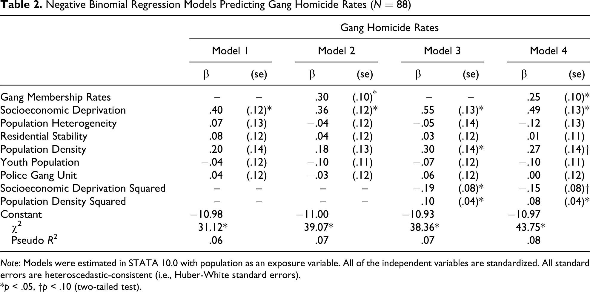
Table 2 displays the results from the negative binomial regression models predicting gang homicide rates.¹⁴ The coefficients can be evaluated in terms of effect size because all variables entered into the models were standardized. To start, bivariate regression models were estimated (not presented) for initial effect size estimates; only coefficients for gang membership rates (β = .39) and socioeconomic deprivation (β = .51) exceeded a magnitude of .30. A model building approach is used to highlight gang membership as an intervening variable because it is expected that structural factors influence the outcome indirectly through gang membership. Of the covariates included in Table 2, socioeconomic deprivation (β = .23, p < .05) and population heterogeneity (β = .39, p < .05) were positively related to rates of gang membership in cities. To the extent that gang membership rates are associated gang homicide rates, socioeconomic deprivation and population heterogeneity exhibit an indirect influence on gang homicide.

Table 2.

Negative Binomial Regression Models Predicting Gang Homicide Rates (N = 88)

	Gang Homicide Rates
	Model 1		Model 2		Model 3		Model 4
	β	(se)	β	(se)	β	(se)	β	(se)
Gang Membership Rates	–	–	.30	(.10)*	–	–	.25	(.10)*
Socioeconomic Deprivation	.40	(.12)*	.36	(.12)*	.55	(.13)*	.49	(.13)*
Population Heterogeneity	.07	(.13)	−.04	(.12)	−.05	(.14)	−.12	(.13)
Residential Stability	.08	(.12)	.04	(.12)	.03	(.12)	.01	(.11)
Population Density	.20	(.14)	.18	(.13)	.30	(.14)*	.27	(.14)†
Youth Population	−.04	(.12)	−.10	(.11)	−.07	(.12)	−.10	(.11)
Police Gang Unit	.04	(.12)	−.03	(.12)	.06	(.12)	.00	(.12)
Socioeconomic Deprivation Squared	–	–	–	–	−.19	(.08)*	−.15	(.08)†
Population Density Squared	–	–	–	–	.10	(.04)*	.08	(.04)*
Constant	−10.98		−11.00		−10.93		−10.97
χ²	31.12*		39.07*		38.36*		43.75*
Pseudo R ²	.06		.07		.07		.08

Note: Models were estimated in STATA 10.0 with population as an exposure variable. All of the independent variables are standardized. All standard errors are heteroscedastic-consistent (i.e., Huber-White standard errors).

*p < .05, †p < .10 (two-tailed test).

Model 1 presents the findings with gang membership excluded from the model. Only socioeconomic deprivation exhibited an influence on gang homicide rates, such that a one standard deviation increase in deprivation corresponded to a .40 standard deviation increase in gang homicide rates—a 20 percent reduction from the bivariate model. Model 2 introduces gang membership rates into the analysis, partially mediating the effect of socioeconomic deprivation by 10 percent (β = .36). As expected, gang membership exhibited an influence on gang homicide rates, where a one standard deviation increase in gang membership rates corresponded to a .30 standard deviation increase in the gang homicide rate. To increase the gang homicide rate by one, a city would need an additional 93 gang members per 10,000 citizens.

Models 3 and 4 explore the nonlinear relationship between two of the structural covariates and gang homicide rates. Prior literature has shown that the effect of socioeconomic deprivation on violence tends to tail off at extreme levels (Krivo and Peterson 2000; McNulty 2001). Further, densely populated neighborhoods and cities are conducive to the processes of gang violence (Decker 1996; Papachristos 2009; Short and Strodtbeck 1965), such that upper tails of the density distribution should correspond to increases in gang homicide rates.¹⁵ Model 3 displays these relationships with gang membership rates absent and the quadratic terms for socioeconomic deprivation and population density operated consistent with expectations. Model 4 presents these relationships with gang membership rates reentered into the model. The magnitude for each of the quadratic terms was reduced by about 20 percent. The results from this final model for the three most influential covariates—gang membership rates, socioeconomic deprivation, and population density—are displayed across standardized scores in Figure 1.

Figure 1

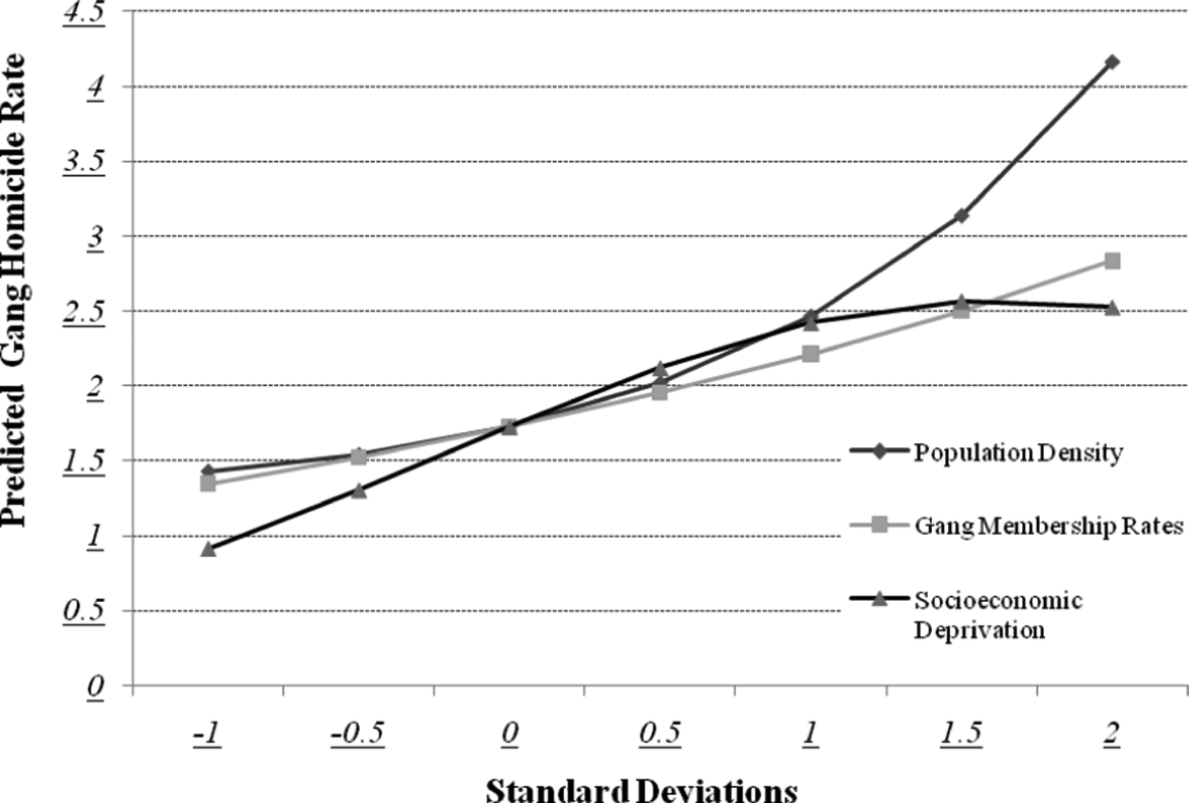
Predicted gang homicide rates across standardized values for key structural covariates

Multivariate Models Predicting Non-Gang and Total Homicide

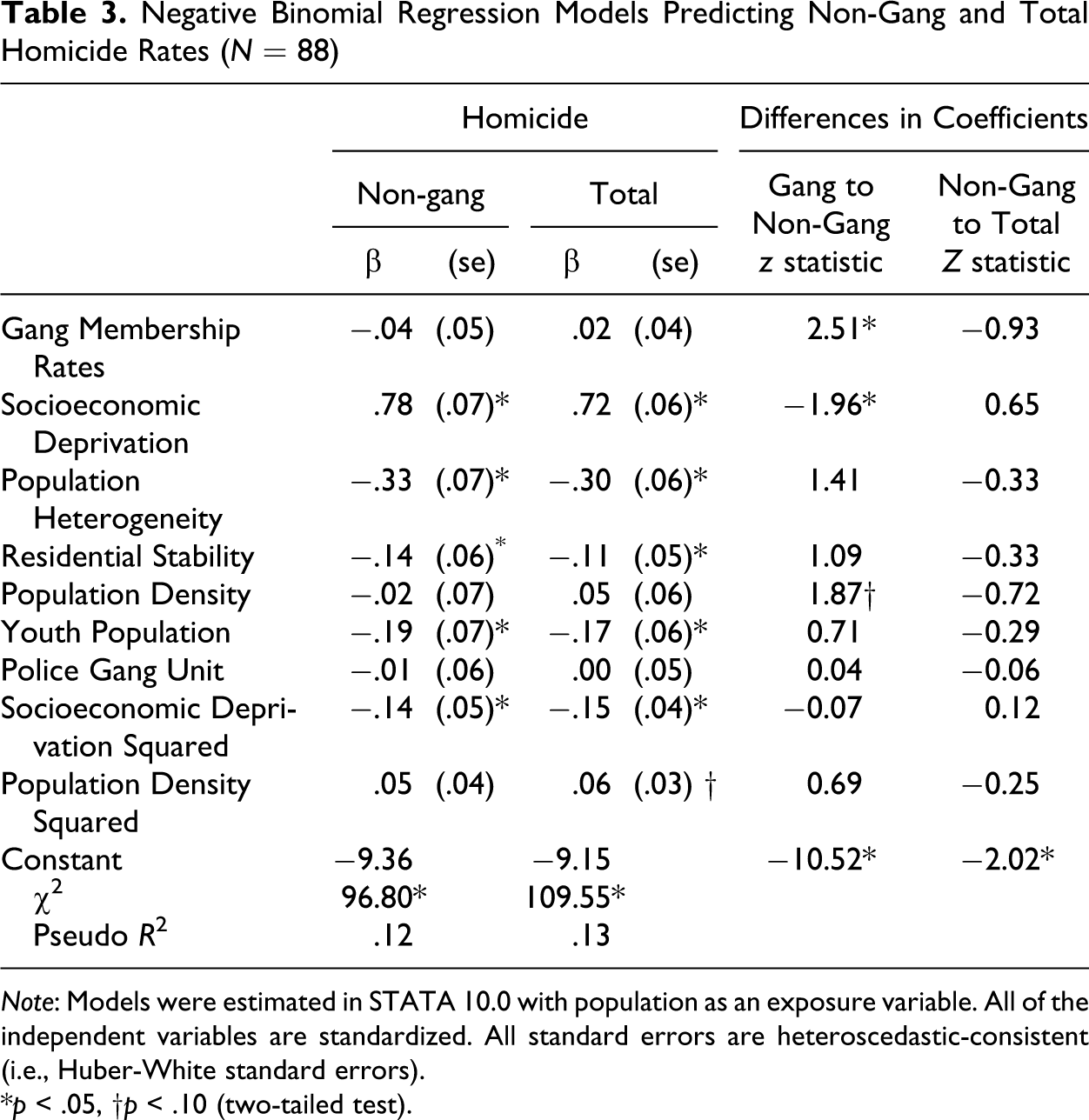
Based on the most fully specified gang homicide model (Table 2, model 4), Table 3 displays the findings for non-gang and total homicides. The statistically significant coefficients identified in these two models are very similar, which is likely a result of non-gang homicide comprising about 80 of the homicides among the sample cities. In particular, socioeconomic deprivation exhibited a strong relationship with both outcomes homicides, demonstrated by a standardized coefficient that exceeded .70. A one standard deviation increase in socioeconomic deprivation corresponds to an additional 7 homicides per 100,000 citizens. The coefficient for population heterogeneity was nearly identical to the bivariate model in terms of sign, significance, and magnitude. Cities with more immigrants, diversity, and Hispanics had lower rates of homicide. Increases in residential stability and youth population corresponded to decreases in homicide rates.¹⁶ Finally, as expected, a statistically significant coefficient for the socioeconomic deprivation quadratic term was observed.

Table 3.

Negative Binomial Regression Models Predicting Non-Gang and Total Homicide Rates (N = 88)

	Homicide				Differences in Coefficients
	Non-gang		Total		Gang to Non-Gang	Non-Gang to Total
	β	(se)	β	(se)	z statistic	Z statistic
Gang Membership Rates	−.04	(.05)	.02	(.04)	2.51*	−0.93
Socioeconomic Deprivation	.78	(.07)*	.72	(.06)*	−1.96*	0.65
Population Heterogeneity	−.33	(.07)*	−.30	(.06)*	1.41	−0.33
Residential Stability	−.14	(.06)*	−.11	(.05)*	1.09	−0.33
Population Density	−.02	(.07)	.05	(.06)	1.87†	−0.72
Youth Population	−.19	(.07)*	−.17	(.06)*	0.71	−0.29
Police Gang Unit	−.01	(.06)	.00	(.05)	0.04	−0.06
Socioeconomic Deprivation Squared	−.14	(.05)*	−.15	(.04)*	−0.07	0.12
Population Density Squared	.05	(.04)	.06	(.03) †	0.69	−0.25
Constant	−9.36		−9.15		−10.52*	−2.02*
χ²	96.80*		109.55*
Pseudo R ²	.12		.13

*p < .05, †p < .10 (two-tailed test).

An equality of coefficients test was used to determine whether the structural conditions associated with gang homicide differed from non-gang homicide (Clogg, Petkova, and Haritou 1995; see also Paternoster et al. 1998). The rightmost columns of Table 3 display the results of the tests. Gang and non-gang coefficients differ statistically for gang membership, socioeconomic deprivation, population density (p = .06), and the intercept. Coefficient differences for gang membership and intercept differences were expected; the former on conceptual grounds and latter on analytic grounds. The socioeconomic deprivation and population density differences are more interesting, however. The effect of socioeconomic deprivation was greater for non-gang homicide than gang homicide, and the effect of population density was greater for gang homicide than non-gang homicide. Finally, after gang homicides were partialled out, with the exception of the intercept, none of the coefficients for the structural covariates differed statistically. The implications of the above findings are discussed in the following section.

Discussion

Land et al. (1990) raised important questions about whether the invariances in the covariates of total homicide rates would be found in homicide rates disaggregated by type. I followed up on that question in the current study, examining the structural covariates of gang homicide in large U.S. cities and whether the conditions associated with gang homicide differed from non-gang homicide. Based on the above findings, four main conclusions emerge from this research.

First, the results support the extension of key “invariant” structural covariates of total homicide—deprivation and population structure—to the context of gang violence (Land et al. 1990; McCall et al. 2010). Several theoretical perspectives inform these findings, including structural control, structural adaptation, and routine activities/opportunity. Cities with greater social and economic deprivation experienced higher rates of gang homicide than their more advantaged counterparts. Structural control explanations emphasize that communities with fewer resources have limited capacities to regulate human behavior (Bursik and Grasmick 1993; Kornhauser 1978; Sampson, Raudenbush, and Earls 1997; Wilson 1987). From this perspective, gangs are naturally occurring deviant social networks that engage in violence as a result of weakened social controls. It is not that these communities are more tolerant of violent gang activities; rather, they lack the collective efficacy to control gangs. Structural adaptation explanations emphasize that environments with limited resources and opportunities for status attainment give way to culture-producing adaptations (Anderson 1999; Cohen 1955; Cloward and Ohlin 1960; Miller 1958). Gangs emerge not only as a vehicle to earn respect and the approval of peers but also as a supposed protective mechanism (Melde, Taylor, and Esbensen 2009). Real and perceived threats elicit group-based responses that result in persistent conflict over time (Decker 1996; Papachristos 2009). Densely populated cities experienced higher rates of gang homicide than sparsely populated cities, consistent with routine activities and opportunity theories (Cohen and Felson 1979). As people are crowded into closer quarters, it increases the probability of interaction between potential offenders and targets in environments absent of guardians, thus resulting in greater rates of victimization. In densely populated cities, the natural routines and movements of gang members are thus structured so as to increase the likelihood that rival gangs cross paths.

Second, this study revealed that while there were similarities across structural covariates of gang and non-gang homicide, there were notable differences as well. Socioeconomic deprivation and population density operated differently in the gang context. The fact that socioeconomic deprivation was more strongly related to non-gang homicide than gang homicide is consistent with a cultural adaptation perspective. Whereas non-gang homicides that are economically or emotionally driven may be more a function of socioeconomic factors, social and cultural processes consisting of retaliatory and institutionalized networks of conflict characterize gang violence. In other words, there are other processes at work that are likely endogenous to socioeconomic deprivation that influence gang homicide rates in cities. Moreover, deceleration at the upper tail of the socioeconomic deprivation distribution—that is, threshold effects—for gang homicide rates suggests that even modest levels of socioeconomic deprivation may be enough to sustain gang-related conflicts in cities. Similarly, population density was more strongly related to gang than non-gang homicide, which is likely a function of the territorial nature of gangs (Brunson and Miller 2009; Decker and Van Winkle 1996; Suttles 1972; Vigil 1988). As the population density of a city increases, it requires gang members to negotiate public space more carefully. Valdez, Cepeda, and Kaplan (2009:295-96) described a situation where gang members were “caught slipping” or had their guard down and were shot at while walking through a rival gang’s territory. While examples such as these are applicable to any city, they are more likely to occur in cities developed for high-density business and housing purposes.

Third, in addition to the main findings described above, increased socioeconomic deprivation and population heterogeneity led to higher rates of gang membership in cities, which in turn led to higher rates of gang homicide. In other words, these structural covariates also had an indirect influence on gang violence, because when larger bodies of gang members are competing for status, dominance, and illicit resources, this should create conflicts that result in violent encounters. Yet, the residual influence of socioeconomic deprivation implies that other processes are at work driving gang homicide rates. To flesh out this finding, a potential avenue for future research is to use the rosters of gang databases as an exposure variable and model the structural correlates of gang homicide victimization. This would provide an idea of how socioeconomic deprivation influences violent gang activity in particular, as well as other structural factors at work in cities more generally, while accounting for indirect influences.

Relatedly, what has become commonly referred to as the Latino or immigrant paradox is the observation that, given their disadvantaged circumstances, these demographic groups engage in crime at lower rates than native-born Americans and immigrants of generations past (Hagan, Levi, and Dinovitzer 2008; Lee, Martinez, and Rosenfeld 2001; Sampson 2008). The null finding in this study is contrary to expectations for researchers of the immigrant-crime nexus and researchers of gang violence, but for different reasons. For the former, a negative relationship would be expected because the protective factor of immigration should extend across all violent crime domains. For the latter, a positive relationship would be expected because, as socially and economically marginalized members of society, immigrant youth would band together to cope with strains and repel antagonisms from more integrated members of the social spectrum. While the indirect relationship suggests the population heterogeneity matters in the context of gangs and violence, the main implication of this finding for the immigration-violent crime debate is that empirical findings may operate differently when violence is disaggregated by category.

Finally, to sufficiently understand gang violence, researchers must cross levels of analysis. The decomposition of gang violence cannot occur at only one unit of analysis; there are macro-, neighborhood-, micro-, and individual-level factors at play in the commission of gang-related violent events (Short 1998). Yet, gang violence has been better understood (and studied) at individual, micro, and neighborhood levels of explanation. To be sure, macro-level factors matter for understanding gang homicide beyond a mere stage where human behavior is acted out. If not, counterfactually, it would be expected that bouts of gang violence would erupt in sparsely populated, middle-class and affluent, and demographically homogeneous neighborhoods and cities. A problem is that while neighborhood-level research—a step closer to structural factors in the causal chain—has expanded significantly over the past quarter-century, gangs have been treated as somewhat of a taboo subject in this line of study. Researchers are oftentimes hesitant to identify gangs as having exogenous influences on social problems (but see Tita, Cohen, and Engberg 2005:272; Tita and Ridgeway 2007), which could be a consequence of the larger debate surrounding structure and culture (Sampson and Bean 2006).

Future research on gang homicide should continue to unpack the neighborhood-macro factors associated with gang violence. In particular, a better empirical understanding of the intervening mechanisms—for example, collective efficacy and community control, cultural adaptations, threat and institutionalized conflict, and gang densities/gang member concentrations—between structural factors and gang homicide is warranted. Also, a more detailed understanding of how the spatial properties of the distribution of people in urban landscapes influences gang homicides would appear to contain broad utility, especially in the context of distance decay and an opportunity framework. At the same time, the nexus between immigration, race and ethnicity, and deprivation is understudied for gangs in general, let alone gang violence. More detailed empirical attention is needed, especially in relation to demographic changes over the past two decades. Finally, the application of cross-level or mixed-model methodology that can account for within- and between-city characteristics to each of these areas of study would create a more accurate picture of the conditions and mechanisms associated with gang homicide.

In conclusion, this study identified socioeconomic deprivation, population density, and gang membership rates as structural covariates of gang homicide in large U.S. cities. Prior to this study, it was well known that gang homicides tended to occur in public settings among marginalized, minority youth situated in socially and economically deprived areas; however, it was unknown whether these findings were distinct from homicide and whether these findings could be generalized beyond specific cities. Data limitations have handicapped the production of knowledge in the homicide literature with respect to gangs (Klein 2005). That said, this study has taken a step toward remedying this issue and placing the findings in the context of homicide in general. Given the institutionalization of gangs and gang violence in urban America, it is necessary that future research further expand this line of study.

Footnotes

Appendix A

Table A1. Factor Loadings for Socioeconomic Deprivation and Population Heterogeneity

	Socioeconomic Deprivation	Population Heterogeneity
Items	Factor Loading	Factor Loading
Population living at or below poverty	.968	–
Unemployed males	.872	–
Income concentrated at extremes (ICE)	−.900	–
Female headed household with children < 18	.902	–
Population receiving public assistance	.757	–
Non-Hispanic African American population	.658	–
Racial/ethnic heterogeneity	–	.586
Immigrant population post-1980	–	.827
Hispanic population	–	.826

Note: Factor loadings were obtained using principal components factor analysis with varimax rotation.

Author’s Note

I would like to thank the editor, Mike Maxfield, and the JRCD reviewers, as well as Scott Decker, Rob Fornango, Charles Katz, Gary Sweeten, and Scott Wolfe, for providing valuable comments on earlier drafts of this article. I thank the National Gang Center for making the data available for this study. An earlier version of this article was presented at the 2010 national conference of the Bureau of Justice Statistics (BJS)/Justice Research and Statistics Association (JRSA) in Portland, Maine, where it was awarded first place in the student paper competition.

Declaration of Conflicting Interests

The author declared no potential conflicts of interest with respect to the research, authorship, and/or publication of this article.

Funding

The author received no financial support for the research, authorship, and/or publication of this article.

Notes

References

Anderson

Elijah

. 1999. Code of the Streets: Decency, Violence and the Moral Life of the Inner City. New York: W.W. Norton and Company.

Avakame

Edem

. 1997. “Urban Homicide: A Multilevel Analysis across Chicago’s Census Tracts.” Homicide Studies 1:338–58.

Bailey

Gary W.

Unnithan

Prabha N.

. 1994. “Gang Homicidens in California: A Discriminant Analysis.” Journal of Criminal Justice 22:267–75.

Baller

Robert D.

Anselin

Luc

Messner

Steven F.

Deane

Glenn

Hawkins

Darnell F.

. 2001. “Structural Covariates of U.S. County Homicide Rates: Incorporating Spatial Effects.” Criminology 39:561–90.

Belsley

David A.

Kuh

Edwin

Welsch

Roy E.

. 2004. Regression Diagnostics: Identifying Influential Data and Sources of Collinearity. Hoboken, NJ: Wiley.

Blau

Peter M.

1977. Inequality and Heterogeneity: A Primitive Theory of Social Structure. New York: Free Press.

Braga

Anthony A.

Kennedy

David M.

Waring

Elin J.

Piehl

Anne Morrison

. 2003. “Problem-Oriented Policing, Deterrence, and Youth Violence: An Evaluation of Boston’s Operation Ceasefire.” Journal of Research in Crime and Delinquency 38:195–225.

Brunson

Rod K.

Miller

Jody

. 2009. “Schools, Neighborhoods, and Adolescent Conflicts: A Situational Examination of Reciprocal Dynamics.” Justice Quarterly 26:183–210.

Bursik

Robert J.

Jr Grasmik

Harold G.

1993. Neighborhoods and Crime: The Dimensions of Effective Community Control. New York: Lexington.

10.

Clogg

C. C.

Petkova

Haritou

. 1995. “Statistical Methods for Comparing Regression Coefficients between models.” American Journal of Sociology 100:1261–93.

11.

Cloward

Richard A.

Ohlin

Lloyd E.

. 1960. Delinquency and Opportunity: A Theory of Delinquent Gangs. New York: Free Press.

12.

Cohen

Albert K.

1955. Delinquent Boys: The Culture of the Gang. New York: Free Press.

13.

Cohen

Lawrence E.

Felson

Marcus

. 1979. “Social Change and Crime Rate Trends: A Routine Activities Approach.” American Sociological Review 44:588–608.

14.

Cohen

Jacqueline

Tita

George

. 1999. “Diffusion in Homicide: Exploring a General Method for Detecting Spatial Diffusion Processes.” Journal of Quantitative Criminology 15:451–93.

15.

Curry

G. David.

Spergel

Irving A.

. 1988. “Gang Homicide, Delinquency, and Community.” Criminology 26:381–407.

16.

Daly

Martin

Wilson

Margo

. 1988. Homicide. New York: Aldine de Gruyter.

17.

Decker

Scott H.

1996. “Collective and Normative Features of Gang Violence.” Justice Quarterly 13:243–64.

18.

Decker

Scott H.

Curry

David G.

. 2002. “Gangs, Gang Homicide, and Gang Loyalty: Organized Crimes or Disorganized Criminals.” Journal of Criminal Justice 30:343–52.

19.

Decker

Scott H.

Pyrooz

David C.

. 2010a. “Gang Violence Worldwide: Context, Culture, and Country.” Pp. 128-55, in Small Arms Survey,2010, edited by Berman

Eric G.

Krause

Keith

LeBrun

Emile

McDonald

Glenn

. Cambridge: Cambridge University Press.

20.

Decker

Scott H.

Pyrooz

David C.

. 2010b. “On the Validity and Reliability of Gang Homicide: A Comparison of Disparate Sources.” Homicide Studies 14:359–76.

21.

Decker

Scott H.

Van Winkle

Barrik

. 1996. Life in the Gang: Family, Friends, and Violence. New York: Cambridge University Press.

22.

FBI. 2010. Crime in the United States. Retrieved October 30, 2010 from http://www.fbi.gov/about-us/cjis/ucr/ucr.

23.

Flewelling

Robert L.

Williams

Kirk R.

. 1999. “Categorizing Homicides: The Use of Disaggregated Data in Homicide Research.” Pp. 96-106 in Homicide: A sourcebook of social research, edited by M. Dwayne Smith and Margaret A. Zahn. Thousand Oaks, CA: Sage.

24.

Gibbs

Jack P.

Martin

Walter T.

. 1962. “Urbanization, Technology, and the Division of Labor: International Patterns.” American Sociological Review 27:667–77.

25.

Gmel

Gerhard

. 2001. “Imputation of Missing Values in the Case of a Multiple Item Instrument Measuring Alcohol Consumption.” Statistics in Medicine 22:2369–81.

26.

Hagan

John

Levit

Ron

Dinovitzer

Ronit

. 2008. “The Symbolic Violence of the Crime-Immigration Nexus: Migrant Mythologies in the Americas.” Criminology and Public Policy 7:95–112.

27.

Henry

Andrew F.

Short

James F.

Jr . 1954. Suicide and Homicide. New York: Free Press.

28.

Hipp

John R.

2007. “Block, Tract, and Levels of Aggregation: Neighborhood Structure and Crime and Disorder as a Case in Point.” American Sociological Review 72:658–80.

29.

Hirschi

Travis

Gottfredson

Michael

. 1983. “Age and the Explanation of Crime.” American Journal of Sociology 89:552–84.

30.

Howell

James C.

1998. Youth Gangs: An Overview. Juvenile Justice Bulletin. Washington DC: Office of Juvenile Justice and Delinquency Prevention.

31.

Howell

James C.

1999. “Youth Gang Homicides: A Literature Review.” Crime and Delinquency 45:208–41.

32.

Huff

C. Ronald

. 1998. Comparing the Criminal Behavior of Youth Gangs and At-Risk Youth. Research in brief. Washington, DC: National Institute of Justice.

33.

Hutson

H. Range

Anglin

Deirdre

Kyriacou

Demetrios

Hart

Joel

Spears

Kelvin

. 1995. “The Epidemic of Gang-Related Homicides in Los Angeles County from 1974 to 1994.” JAMA 273:1031–6.

34.

Jöreskog

K. G.

Sörbom

Dag

. 1996. Prelis 2 User’s Reference Guide (3rd ed). Chicago: Scientific Software International.

35.

Katz

Charles M.

Ballance

Steve

Britt

Chester

. 2005. Examining the Reliability of the National Youth Gang Survey. Presentation at the Western Society of Criminology annual conference, Honolulu, HI.

36.

Katz

Charles M.

Schnebly

Stephen M.

. 2010. “Neighborhood Variation in Gang Member Concentrations.” Crime and Delinquency. 57:377–407.

37.

Katz

Charles M.

Webb

Vincent J.

. 2006. Policing Gangs in America. Cambridge: Cambridge University Press.

38.

Katz

Charles M.

Webb

Vincent J.

Schaefer

David

. 2000. “The Validity of Police Gang Intelligence Lists: Examining Differences in Delinquency between Documented Gang Members and Non-Documented Delinquent Youth.” Police Quarterly 3:413–37.

39.

Klein

Malcolm W.

1995. The American Street Gang: Its Nature, Prevalence, and Control. New York: Oxford University Press.

40.

Klein

Malcolm W.

2005. “The Value of Comparisons in Street Gang Research.” Journal of Contemporary Criminal Justice 21:135–52.

41.

Klein

Malcolm W.

Maxson

Cheryl L.

. 2006. Street Gang Patterns and Policies. New York: Oxford University Press.

42.

Kornhauser

Ruth R.

1978. Social Sources of Delinquency: An Appraisal of Analytic models. Chicago: University of Chicago Press.

43.

Kovandzic

Tomislav V.

Vieraitis

Lynne M.

Yeisley

Mark R.

. 1998. “The Structural Covariates of Urban Homicide: Reassessing the Impact of Income Inequality and Poverty in the Post-Reagan Era.” Criminology 36:569–600.

44.

Krivo

Lauren J.

Peterson

Ruth D.

. 2000. “The Structural Context of Homicide: Accounting for Racial Differences in Process.” American Sociological Review 65:547–59.

45.

Kubrin

Charis E.

2003. “Structural Covariates of Homicide Rates: Does Type of Homicide Matter?” Journal of Research in Crime and Delinquency 40:139–70.

46.

Kubrin

Charis E.

Herting

Jerald

. 2003. “Neighborhood Correlates of Homicide Trends: An Analysis Using Growth-Curve Modeling.” Sociological Quarterly 44:329–50.

47.

Kubrin

Charis E.

Wadsworth

Tim

. 2003. “Identifying the Structural Correlates of African-American Killings: What can we Learn from Data Disaggregation?” Homicide Studies 7:3–35.

48.

Kyriacou

Demetrios N.

Range Hutson

Anglin

Deirdre

Peek-Asa

Corinne

Kraus

Jess F.

. 1999. “The Relationship between Socioeconomic Factors and Gang Violence in the City of Los Angeles.” Journal of Trauma 46:334–39.

49.

Land

Kenneth C.

McCall

Patricia L.

Cohen

Lawrence E.

. 1990. “Structural Covariates of Homicide Rates: Are there any Invariances across Time and Social Space.” American Journal of Sociology 95:922–63.

50.

Langton

Lynn

. 2010. Gang Units in Large Local Law Enforcement agencies,2007. Washington, DC: U.S. Department of Justice, Office of Justice Programs, Bureau of Justice Statistics.

51.

Lee

Matthrew T.

Martinez

Ramiro

Jr Rosenfeld

Richard

2001. “Does Immigration Increase Homicide? Negative Evidence from Three Border Cities.” Sociological Quarterly 42:559–80.

52.

Little

Roderick J.

Yosef

Matheos

Cain

Kevin C.

Nan

Bin

Harlow

Sioban D.

. 2008. “A Hot-Deck Multiple Imputation Procedure for Gaps in Longitudinal Data on Recurrent Events.” Statistics in Medicine 27:103–20.

53.

Mares

Dennis

. 2010. “Social Disorganization and Gang Homicides in Chicago: A Neighborhood Level Comparison of Disaggregated Homicides.” Youth Violence and Juvenile Justice 8:38–57.

54.

Maxson

Cheryl L.

1999. “Gang Homicide: A Review and Extension of the Literature.” Pp. 239-56 in Homicide: A sourcebook of social research, edited by M. Dwayne Smith and Margaret A. Zahn. Thousand Oaks, CA: Sage.

55.

Maxson

Cheryl L.

Curry

David G.

Howell

James C.

. 2002. “Youth Gang Homicides in the United States in the 1990s.” Pp. 107-38 in Responding to Gangs: Evaluation and Research, edited by Winifred L. Reed and Scott H. Decker. Washington, DC: National Institute of Justice.

56.

Maxson

Cheryl L.

Gordon

Margaret A.

Klein

Malcolm W.

. 1985. “Differences between Gang and Nongang Homicides.” Criminology 23:209–22.

57.

Maxson

Cheryl L.

Klein

Malcolm W.

. 1990. “Defining Gang Homicide: Twice as Great, or Half as Great?” Pp. 71-100 in Gangs in America, edited by C. Ron Huff. Newbury Park, CA: Sage.

58.

McCall

Patricia

Land

Kenneth C.

Parker

Karen F.

. 2010. “An Empirical Assessment of What We Know about Structural Covariates of Homicide Rates: A Return to a Classic 20 Years Later.” Homicide Studies 14:219–43.

59.

McNulty

Thomas L.

2001. “Assessing the Race-Violence Relationship at the Macro Level: The Assumption of Racial Invariance and the Problem of Restricted Distributions.” Criminology 39:467–90.

60.

Melde

Chris

Taylor

Terrance J.

Esbensen

Finn-Aage

. 2009. “ ‘I Got Your Back': Examining the Protective Function of Gang Membership in Adolescence.” Criminology 47: 565–594.

61.

Miller

Jody

Decker

Scott H.

. 2001. “Young Women and Gang Violence: Gender, Street Offending, and Violent Victimization in Gangs.” Justice Quarterly 18:115–40.

62.

Morenoff

Jeffrey D.

Sampson

Robert J.

Raudenbush

Stephen W.

. 2001. “Neighborhood Inequality, Collective Efficacy, and the Spatial Dynamics of Urban Violence.” Criminology 39:517–60.

63.

National Youth Gang Center. 2009. National Youth Gang Survey Analysis. Retrieved November 29, 2009, from http://www.nationalgangcenter.gov/Survey-Analysis.

64.

Osgood

D. Wayne

. 2000. “Poisson-Based Regression Analysis of Aggregate Crime Rates.” Journal of Quantitative Criminology 16:21–43.

65.

Parker

Karen F.

2004. “Industrial Shift, Polarized Labor Markets and Urban Violence: Modeling the Dynamics between the Economic Transformation and Disaggregated Homicide.” Criminology 42:619–46.

66.

Parker

Karen F.

McCall

Patricia L.

Land

Kenneth C.

. 1999. “Determining the Social-Structural Predictors of Homicide: Units of Analysis and Related Methodological Concerns.” Pp. 107-24 in Homicide: A Sourcebook of Social Research, edited by M. Dwayne Smith and Margaret A. Zahn. Thousand Oaks, CA: Sage.

67.

Papachristos

Andrew V.

2009. “Murder by Structure: Dominance Relations and the Social Structure of Gang Homicide.” American Journal of Sociology 115:74–128.

68.

Papachristos

Andrew V.

Kirk

David S.

. 2006. “Neighborhood Effects on Street Gang Behavior.” Pp. 63-85 in Studying Youth Gangs, edited by James F. Short and Lorine Hughes. Lanham, MD: Altamira.

69.

Paternoster

Raymond

Brame

Robert

Mazerolle

Paul

Piquero

Alex R.

. 1998. “Using the Correct Statistical Test for the Equality of Regression Coefficients.” Criminology 36:859–66.

70.

Pizarro

Jesenia M.

2008. “Reassessing the Situational Covariates of Homicide: Is there a Need to Disaggregate?” Homicide Studies 12:323–49.

71.

Pizarro

Jesenia

McGloin

Jean Marie

. 2006. “Explaining Gang Homicides in Newark, New Jersey: Collective Behavior or Social Disorganization?” Journal of Criminal Justice 34:195–207.

72.

Podsakoff

Philip M.

Organ

Dennis W.

. 1986. “Self-Reports in Organizational Research: Problems and Prospects.” Journal of Management 12:531–44.

73.

Pyrooz

David C.

Fox

Andrew M.

Decker

Scott H.

. 2010. “Racial and Ethnic Heterogeneity, Economic Disadvantage, and Gangs: A Macro-Level Study of Gang Membership in Urban America.” Justice Quarterly 27:867–93.

74.

Pyrooz

David C.

Wolfe

Scott E.

Spohn

Cassia

. 2011. “Gang-Related Homicide Charging Decisions: An Analysis of the Implementation of a Specialized Prosecution Unit in Los Angeles.” Criminal Justice Policy Review 22:3–26.

75.

Rosenfeld

Richard

Bray

Timothy M.

Egley

Arlen

. 1999. “Facilitating Violence: A Comparison of Gang-Motivated, Gang-Affiliated, and Non-Gang Youth Homicides.” Journal of Quantitative Criminology 15:495–516.

76.

Sampson

Robert J.

2008. “Rethinking Crime and Immigration.” Contexts 7:28–33.

77.

Sampson

Robert J.

Bean

Lydia

. 2006. “Cultural Mechanisms and Killing Fields: A Revised Theory of Community-Level Racial Inequality.” Pp. 8-38 in The Many Colors of Crime: Inequalities of Race, Ethnicity, and Crime in America, edited by Ruth D. Peterson, Lauren J. Krivo, and John Hagan. New York: New York University Press.

78.

Sampson

Robert J.

Raudenbush

Stephen W.

Earls

Felton

. 1997. “Neighborhoods and Violent Crime: A Multilevel Study of Collective Efficacy.” Science 277:918–24.

79.

Sanders

James B.

1994. Gangbangs and Drive-Bys: Grounded Culture and Juvenile Gang Violence. Hawthorne, NY: Aldine de Gruyter.

80.

Short

James F.

, Jr. 1998. “The Level of Explanation Problem Revisited: The American Society of Criminology 1997 Presidential Address.” Criminology 36:3–36.

81.

Short

James F.

Jr Strodtbeck

Fred L.

. 1965. Group Process and Gang Delinquency. Chicago: University of Chicago Press.

82.

Smith

M. Dwayne

Zahn

Margaret A.

. 1999. Homicide: A Sourcebook of Social research. Thousand Oaks, CA: Sage.

83.

Steffensmeier

Darrell

Haynie

Dana

. 2000. “The Structural Sources of Urban Female Violence in the United States: A Macrosocial Gender-Disaggregated Analysis of Adult and Juvenile Homicide Offending Rates.” Homicide Studies 4:107–34.

84.

Suttles

Gerald D.

1972. The Social Construction of Communities. Chicago: University of Chicago Press.

85.

Tita

George

Abrahamse

Allan

. 2004. Gang Homicide in LA,1981-2001. Sacramento, CA: California Attorney General’s Office.

86.

Tita

George

Cohen

Jacqueline

Engberg

John

. 2005. “An Ecological Study of the Location of Gang ‘Set Space.’” Social Problems 52: 272–99.

87.

Tita

George

Ridgeway

Greg

. 2007. “The Impact of Gang Formation on Local Patterns of Crime.” Journal of Research on Crime and Delinquency 44:208–37.

88.

United States Department of Justice. Bureau of Justice Statistics. 2000. Law Enforcement Management and Administrative Statistics (LEMAS). Sample Survey of Law Enforcement Agencies [Computer file]. ICPSR03565-v2. Ann Arbor, MI: Inter-university Consortium for Political and Social Research [distributor], 2008-12-04. doi:10.3886/ICPSR03565.

89.

Valdez

Avelardo

Cepeda

Alice

Kaplan

Charles

. 2009. “Homicidal Events among Mexican American Street Gangs: A Situational Analysis.” Homicide Studies 13:288–306.

90.

Vigil

James D.

1988. Barrio Gangs: Street Life and Identity in Southern California. Austin: University of Texas Press.

91.

Wadsworth

Tim

Kubrin

Charis E.

. 2004. “Structural Factors and Black Interracial Homicide: A New Examination of the Causal Process.” Criminology 42:647–72.

92.

Williams

Kirk R.

Flewelling

Robert L.

. 1988. “The Social Production of Criminal Homicide: A Comparative Study of Disaggregated Rates in American Cities.” American Sociological Review 53:421–31.

93.

Wilson

William J.

1987. The Truly Disadvantaged: The Inner City, the Underclass, and Public Policy. Chicago: University of Chicago Press.

94.

Wirth

Louis

. 1938. “Urbanism as a Way of Life.” American Journal of Sociology 44:1–24.

95.

Wolfgang

Marvin E.

1958. Patterns in Criminal Homicide. Philadelphia, PA: University of Pennsylvania Press.