
Abstract
Objectives:
Recent work has debated which geographic scale is most relevant to understanding the clustering of crime and disorder across a city. This study introduces nested Gini coefficients that help answer this question by disentangling concentrations of crime at multiple scales in a single city while also controlling for artifacts of arithmetic and urban form.
Methods:
The study examines six indices of crime and disorder drawn from requests for government services received by the City of Boston in 2011 for addresses (N = 98,355) nested in street segments (N = 13,048) nested in census tracts (N = 178). Nested Gini coefficients assessed the average concentration at each level independent of the higher geographic unit (e.g., the streets of a single tract).
Results:
Concentrations were greatest at addresses, then at streets, and then at tracts. Compared to whole-city calculations, they showed equal or greater levels of concentration of crime and disorder for addresses, but lower concentrations for streets. Controlling for the number of locations on a street or in a tract also markedly diminished concentrations.
Conclusions:
The findings indicate a continued need to explain concentrations of crime, especially at localized geographic scales.
One of the basic motivations for urban criminology is the observation that crime and disorder are unevenly distributed across the urban landscape. Over the years, though, multiple perspectives have emphasized the importance of one geographic scale of analysis or another for observing and understanding this variation. Classical thought emphasized “high-risk neighborhoods” (e.g., Park, Burgess, and McKenzie [1925] 1984; Sampson 2012; Shaw and McKay [1942] 1969), but recent trends have redirected attention to more localized contexts, including “hotspot streets” (e.g., Andresen and Malleson 2011; Braga, Papachristos, and Hureau 2010; Weisburd 2015; Weisburd, Groff, and Yang 2012) and “problem properties” (or “hotdots”; Farrell and Pease 2001; Johnson, Bowers, and Hirschfield 1997; O’Brien and Winship 2017; Sherman, Gartin, and Buerger 1989). Although considerable work has provided evidence for the relevance of each of these geographic scales, only a few studies have analyzed them simultaneously in order to compare their relative levels of concentration. This is a particularly tricky task because these geographic scales are inherently interdependent—addresses sit on streets which lie within neighborhoods—creating the need for analytic approaches that can disentangle concentrations at one level from the others.
The current study introduces a new methodological approach of nested Gini coefficients to disentangle concentrations of crime and disorder across multiple geographic scales. It applies this technique to a database of requests for government services (i.e., 911 and 311 calls) from Boston, MA, to examine the relative concentration of six types of crime and disorder at addresses, street segments, and census tracts. Gini coefficients quantify inequality in a distribution, but nesting them within geographic levels makes it possible to assess concentrations at each geographic scale independently of concentrations that exist at higher levels of aggregation (e.g., separating concentrations at addresses from concentrations across the streets that contain them). The study will also leverage additional techniques to address two other challenges to the interpretation of concentrations of crime and disorder: (1) the arithmetic consequences of the rarity of crime, which can inflate Gini estimates, and (2) aspects of urban form that can influence the distribution of crime and disorder, including land use and the density of locations where such events might occur. Altogether, the approach permits a comprehensive assessment of concentration at all three levels, controlling for multiple arithmetic and compositional artifacts that have occluded previous work. Before the presentation of data and analyses, the proceeding sections summarize in greater depth how the history of the study of crime concentrations and the statistical and conceptual challenges facing their examination shape the current study.
Concentrations of Crime: A Methodological Challenge
Scholars have sought to understand the uneven distribution of outcomes across a city’s neighborhoods for at least 150 years (e.g., Booth 1903; Mayhew 1862), making it one of the oldest themes in urban science. In the early twentieth century, the Chicago School of Sociology took particular aim at this subject, probing inequalities in crime, health, and education across communities (Park and Burgess 1925; Shaw and McKay [1942] 1969). This work has since provided the conceptual basis for decades of research on the social, demographic, and physical features of neighborhoods that can influence local levels of crime (Browning, Soller, and Jackson 2015; Cohen et al. 2000; Gibson et al. 2010; Kawachi and Berkman 2003; Leventhal and Brooks-Gunn 2000; Raudenbush and Sampson 1999; Sampson, Raudenbush, and Earls 1997). A more recent line of work, however, has highlighted the extent to which microplaces, or streets and addresses, contribute to the distribution of outcomes, most notably crime and disorder, across the city. This “criminology of place” has debunked the assumption that neighborhoods are homogenous regions, demonstrating that many streets in high-crime neighborhoods actually experience little crime, and that, conversely, there are high-crime streets in low-crime neighborhoods.
Criminology of place began with two studies in the late 1980s in two different cities, each demonstrating that ∼3 percent of addresses accounted for 50 percent of crime events (Pierce, Spaar, and Briggs 1988; Sherman et al. 1989). This discovery was revelatory at a time when neighborhoods were the primary focus for urban criminology. In the years that have followed, research in this area has largely converged upon “hotspot” street segments as the geographic scale of greatest interest, finding that, across cities, 4–6 percent of streets consistently generate 50 percent of crime events (Andresen and Malleson 2011; Braga et al. 2010; Weisburd 2015). Nonetheless, there has also been evidence that concentrations exist at an even more granular level, with a corresponding literature on repeat victimization identifying “hotdot” addresses that experience multiple crimes, most notably burglaries (e.g., Farrell and Pease 2001; Johnson et al. 2007; Trickett et al. 1992). Similarly, an additional recent study replicated the earliest findings of criminology of place by showing that <2 percent of addresses accounted for 50 percent of events across six categories of crime and disorder in a single city (O’Brien and Winship 2017). The consistency of these findings across locales and types of crime has both inspired and further validated Weisburd’s (2015) law of concentration of crime: That for a given microgeographic unit, there is a narrow bandwidth of percentages for a defined cumulative proportion of crime events.
Criminology of place has successfully demonstrated that “microplaces matter,” offering a counterpoint to the neighborhood-centric perspective that characterized the field. That said, affirming the importance of street segments and addresses is only a first step; a comprehensive understanding of concentrations of crime requires the simultaneous consideration of all three geographic levels and their relative contributions to the distribution of crime across the city. Some early work examined streets and neighborhoods together, mainly to reach the conclusion that streets offer additional information that is not available through an exclusive focus on neighborhoods (Andresen and Malleson 2011; Groff, Weisburd, and Yang 2010). This, however, is not the same as evaluating how much information each level contributes. We might then consider three main methodologies to target this question more directly. First, the most popular approach to concentrations of crime has been the use of proportions, for example, determining what proportion of units accounts for 50 percent of crime events. While evocative, it has not been used for comparisons as it does not support formal statistical testing. Second, multilevel models nest units from two or more geographic scales within each other (e.g., addresses on streets in neighborhoods) and can partition variance across these levels, thereby describing the relative contribution of each to the total variation in crime and disorder across the city. This technique has been used by a handful of studies (e.g., Boessen and Hipp 2015; Schnell, Braga, and Piza 2017; Steenbeek and Weisburd 2016; Tseloni 2006), though only one has examined addresses, streets, and neighborhoods simultaneously (O’Brien and Winship 2017). Third, the Gini coefficient offers a standardized measure of inequality based on the Lorenz curve, which plots the proportion of a given quantity on the y-axis (often wealth, though in this case crime and disorder events) held by the x percent of the population with the lowest amount of that quantity (i.e., the fewest crime and disorder events). The Gini coefficient then quantifies inequality as the total distance between the points on the Lorenz curve and the line of perfect equality (y = x). 1 Bernasco and Steenbeek (2017) have suggested that the Gini coefficient might be used for direct comparisons across cities, especially with the calculation of standard errors via bootstrapping. The same approach could be repurposed to compare geographic scales in a single city.
Multilevel models and Gini coefficients offer two potential tools for comparing concentrations of crime across geographic scales, but neither is fully equipped in its traditional form to handle the challenges that this question poses, which we can categorize into three groups: (1) the difficulty of disentangling and then comparing concentrations at multiple geographic scales, (2) statistical artifacts that arise from the rare nature of crime, and (3) the possibility that concentrations of crime might result from the varied organization of the city. By examining each further, it might be possible to develop a modified methodology that can effectively answer the question at hand.
Disentangling nested geographic scales
Comparing levels of concentration across geographic levels within a single city is problematic. Essentially, such an analysis distributes the same set of events over geographic units that are nested within each other, meaning the level of concentration at one level is dependent on others. This makes it difficult to disentangle which levels are contributing most strongly. For example, take a city where crime rates are unevenly distributed across neighborhoods. Suppose then that the crimes within each neighborhood are distributed perfectly evenly across its streets. In this case, it would be inaccurate to attribute any of the distribution of crime to streets. Nonetheless, if streets are analyzed directly, they will appear to exhibit just as much concentration as neighborhoods because they are merely a more granular depiction of the same inequalities. Put in terms of basic arithmetic, shifting to a more localized geographic scale means distributing the same number of events across a larger number of units. Thus, concentrations will inevitably look greater. The more appropriate question, then, is how much of the concentration of crime observed across streets is greater than what would be expected given known disparities between neighborhoods?
Disentangling each geographic level’s contribution to the distribution of crime requires analytic techniques that attend to nesting, which is the specialty of multilevel models (Raudenbush and Bryk 2002). Multilevel models decompose variance across two or more levels by only analyzing units at one level in relation to other units in the same “nest” or containing unit of the next highest geographic level. For example, it compares each street to other streets in the same tract and then compares tracts to each other. This permits an estimation of the proportion of overall variation in crime for which each level is responsible. An important caveat, however, is that these comparisons will be strictly relative because the total percentage of variance must add up to 100 percent. Consequently, the assessment of concentration at each level is contingent on the amount of variance at the others; if one level has particularly high levels of concentration, it will make concentrations at other levels look quite small even if they are noteworthy in an absolute sense. The relative nature of this metric also makes comparisons of concentrations across cities impossible. In contrast, though the Gini coefficient does calculate absolute levels of concentration that are inherently comparable across scales and cities, it does not take into account nesting. In this sense, neither is perfectly suited to this problem. Given the complementary strengths and weaknesses of multilevel models and the Gini coefficient, it is possible that an approach that combines the two would be most effective. We explore what this might look like further below.
Statistical artifacts
The rarity of crime and disorder creates an arithmetic difficulty for analyzing their concentration, hindering the interpretation of the most suitable methodologies. In particular, many addresses and street segments do not generate any crime and disorder. This is problematic for multilevel models because the large number of zeroes at lower levels of aggregation exaggerates the overall variation. Indeed, O’Brien and Winship (2017) found that addresses accounted for 95–99 percent of the variance in six categories of crime and disorder, reflecting the fact that the vast majority of addresses in any street or tract had zero events, whereas others had dozens. Similarly, if there are more units then events, the Gini coefficient will generate an inflated estimate of inequality. For example, if there are three units and only one event, then it must have occurred at only one unit. According to the Gini, this is a maximally unequal distribution, with one unit accounting for 100 percent of events, but it is also technically the most equitable distribution possible. Bernasco and Steenbeek (2017) have forwarded a modified Gini coefficient that solves this issue by comparing a distribution to the minimum amount of inequality possible with the given number of units and events.
Analyses of crime concentrations to date have failed to address a second arithmetic consideration. Crime and disorder are events and therefore would be expected to have a Poisson distribution if distributed randomly. 2 A Poisson distribution is by definition uneven. Particularly for phenomena like crime for which events are rare relative to the number of units, the distribution features an overrepresentation of cases with very few events and a long tail with a small number of cases with many events. Although such a distribution intuitively appears to be highly unequal, it is the expected outcome of the random distribution of events. Thus, research on crime and place has made the mistake of implicitly comparing levels of concentrations to a uniform distribution rather than the expected distribution, given a particular number of events distributed across a specified number of units. Again, the Gini coefficient lends itself to simple simulations that could estimate the expected level of unequal distribution, enabling a true comparison between the observed distribution and its deviation from true randomness.
Artifacts of urban form
One of the founding premises of criminology of place, rooted in routine activities theory (Cohen and Felson 1979), is that aspects of urban form, like land usage (e.g., Bichler, Schmerler, and Enriquez 2013; Browning et al. 2010; Eck 1994; Kinney et al. 2008; Stucky and Ottensmann 2009) or proximity to transportation hubs (e.g., Block and Davis 1996; Caplan, Kennedy, and Miller 2011; Smith and Clarke 2000), can create localized concentrations of crime. For example, detached housing attracts more burglaries (Bowers and Johnson 2005) and street segments with businesses tend to attract more robberies (Smith, Frazee, and Davison 2000). It is possible, in turn, that global estimates of concentration of crime at a particular geographic scale are driven in part by the clustering of such characteristics. This has been visible in two studies on street-level patterns in crime that have found that hotspots tend to form linear clusters along thoroughfares (Curman, Andresen, and Brantingham 2015; Groff et al. 2010). This would suggest that the potential for crime is concentrated at the neighborhood level and then further concentrated within the neighborhood at places that share certain critical features, in this case, a main street with lots of businesses. Thus, it is necessary to consider such factors in order to determine the extent to which they are responsible for clustering at each geographic scale.
There is a need to consider features of urban form as covariates, but we might divide them into two groups based on their interpretation. First, there is the sheer size of a geography or the number of locations where crime might occur therein (e.g., addresses on a street). This would seem to be inherent to clustering; for example, might some streets that appear to be hotspots just have many more addresses than usual? It is important to note that studies on the concentration of crime often have not accounted for this potential confound. 3 The second set of features of interest is land use and other aspects of design and zoning that can shape routine activities. These features are substantively interesting as they might influence crime, yet there is a case for quantifying their impact on estimates of concentrations at different geographic scales. To illustrate, suppose that crime within a neighborhood does concentrate on major thoroughfares, ignoring this fact would obscure differences in crime across neighborhoods by attributing much of the clustering to individual street segments within those neighborhoods. A complete analysis would need to assess how much land use characteristics influence estimated concentrations.
Given that some aspects of urban form are covariates of crime, the most logical approach to addressing them would be through multilevel models. Multilevel models explicitly estimate the effect of parameters at two or more levels on the average outcome at the lowest level. This in turn accounts for the number of locations for all included geographic scales. For example, if addresses are nested on streets and within tracts, the model estimates the amount of crime or disorder at the typical address on the typical street in the typical neighborhood and estimates the extent to which particular features predict an address (or set of addresses on a street or set of addresses in a tract) to have more or less crime or disorder than said typical address. That said, it is important to note that a multilevel model that nests streets within tracts would not naturally account for the number of addresses on a street unless that value were included as a covariate in the model. Turning to features of land use, they could be included in multilevel models as predictors, though only a few studies comparing the variance of crime at multiple geographic scales have done so (Boessen and Hipp 2015; O’Brien and Winship 2017). Even in those two exceptions, however, the authors controlled for such features but did not quantify the extent to which they increased or decreased the relative variance present at each geographic level. Although multilevel models would then appear to be a good solution for this particular challenge, it would still be difficult to compare levels of concentration across levels, as noted above. It may again be that the relative strengths of multilevel models and Gini coefficients would enable the ideal methodology.
A Proposed Solution: Nested, Modified Gini Coefficients
As noted, a methodology that combined the strengths of multilevel models and Gini coefficients might overcome the three main analytic challenges for quantifying levels of concentration of crime at multiple geographic scales. Because the goal is to calculate absolute levels of concentration that can be directly compared both within and across cities, the Gini coefficient will need to act as the base analytic technique. In order to disentangle levels of concentration across multiple geographic scales, the study builds on the logic of multilevel models to introduce nested Gini coefficients. Just as multilevel models compare addresses within streets or streets within tracts to assess variance and covariates at lower levels of aggregation, this approach will examine the distribution of events across the units contained in a single, higher-level unit. Figure 1 illustrates this approach for physical disorder and deterioration to private spaces (measured through 311 reports; see Current Study and Methods) in a single tract in Boston, MA. We can see that this tract’s level of physical disorder is on the high end (172 reports) of a moderately imbalanced distribution (G = .46 for events across tracts). By zooming into this single tract, we observe that those 172 reports of physical disorder are also distributed quite unevenly across its streets (G’ = .80). Narrowing in further on one of the more disorderly streets in the tract (15 reports) reveals, again, that the events are concentrated at only a few addresses (G’ = .83).

An illustration of nested concentrations of crime and disorder at multiple geographic scales through the statistical and spatial distribution of reports of private neglect through Boston’s 311 system for (a and b) census tracts, (c and d) the streets of a single, high-disorder census tract, and (e and f) the addresses of a single high-disorder street in that tract. Histograms also indicate concentration as measured by the Gini coefficient. Histograms utilize a logarithmic scale on the x-axis for easier interpretability; 0s are included in the first bar on the left.
The specific set of measures of concentration depicted in Figure 1 is anecdotal, but it demonstrates a methodology that might be scaled to the entire city for more robust interpretation. For example, calculating the mean of Gini coefficients for events within every tract in the city would estimate the typical level of concentration of physical disorder on streets while accounting for its uneven distribution across tracts. The same logic can be applied to addresses within streets. Thus, the nested Gini coefficients would generate standardized estimates of concentration at each geographic scale independent of the distribution at higher levels of aggregation.
There remain, however, the second and third analytic challenges described thus far: statistical artifacts, and aspects of urban form. For the first, Bernasco and Steenbeek (2017) have proposed the modified Gini (G’) to handle the rarity of crime and disorder, specifically addressing situations in which units outnumber events. That will be used in the following analysis whenever necessary. For the latter, multilevel models again prove valuable. After running the initial Gini analysis, multilevel models with various covariates at all three geographic scales, including land use and the density of locations, will predict counts of events. The residuals from these models will reflect the number of events above or below expected for a given unit, independent of these basic characteristics. These adjusted counts will then be the basis for a second set of Gini coefficients, allowing us to quantify the extent to which aspects of urban form are responsible for crime concentrations for each geographic scale. Altogether, the use of nested, modified Gini coefficients to analyze counts of crime and disorder adjusted for aspects of urban form will permit a robust comparison of concentration across levels.
The Current Study
The current study implements the proposed analytic approach to disentangle levels of concentration of crime across the City of Boston at three different geographic scales: addresses, street segments, and neighborhoods (approximated with census tracts). 4 The novel approach will be more robust for comparing concentrations of crime at multiple geographic scales than recent studies that have relied on multilevel models. It also will quantify the impact of urban form on relative levels of concentration, something that these previous studies have not done. In doing so, the study actually uses the database from one of these previous multilevel studies (O’Brien and Winship, 2017), an archive of records from the City’s 911 and 311 systems, which receive and compile requests for nonemergency (e.g., graffiti removal) and emergency (e.g., shooting) government services, respectively. It leverages six categories of crime and disorder developed by other previous work with these data. These are defined as the combination of particular case types, including physical disorder in private and public spaces, social disorder in private and public spaces, and violent crime with and without guns (O’Brien and Sampson 2015; O’Brien, Sampson, and Winship 2015). The records will be analyzed in conjunction with the Geographical Infrastructure for the City of Boston (O’Brien and Gomory 2017), a multilevel database that organizes the geography of the city at 17 geographic scales. It includes basic descriptors of urban form at each of the three levels of interest while also providing the capacity for nesting levels within each other (e.g., addresses on street segments within tracts), which is essential to the analysis that follows.
Methods and Data
Data Sources and Measures
The study utilizes the archive of requests for service received by the City of Boston’s 311 system and dispatches made by the 911 system in 2011. For the 311 system, this includes requests received by hotline as well as associated web platforms (e.g., smart-phone application). During 2011, the City received 153,731 unique requests through the 311 system 5 and made 560,393 911 dispatches. Of these, 141,062 311 requests and 525,183 911 dispatches referenced an address or intersection that could be uniquely identified in the list of known locations maintained by the City of Boston (see Units of Analysis section), reflecting the equivalent of geocoding rates of 92 percent and 94 percent, respectively. 6 Data were further limited to those events attributed to an address (i.e., excluding intersections; 114,029 311 reports and 491,488 911 dispatches). Importantly, each location is where services were required, not necessarily the location from which the request was made. Each system utilizes a standardized list of case types to categorize all requests at the time of receipt, capturing the nature of the issue and the services required. All records also contain the date and time the request was received.
Previous work with Boston’s 311 and 911 archives used confirmatory factor analysis to develop groupings of case types that act as indices of disorder and crime; 7 311 reports provided two indices of physical disorder (O’Brien et al. 2015): private neglect, comprised of cases referencing housing issues (e.g., rodent infestation), uncivil use of private space (e.g., illegal rooming house and illegal parking on yard), and problems with big buildings (i.e., apartments and condos), and public denigration, comprised of cases reflecting graffiti and the improper disposal of trash. The 911 dispatches provided two indices of social disorder and two indices of violent crime (O’Brien and Sampson 2015). The indices of social disorder were public social disorder, such as panhandlers, drunks, and loud disturbances, and private conflict arising from personal relationships (e.g., domestic violence). The indices of violent crime were public violence, which did not involve a gun (e.g., fight), and prevalence of guns, as indicated by shootings or other incidents involving guns. Table 1 reports constituent case types for each index and their frequencies for 2011.
Case Types Composing the Indices of Physical Disorder (311 Reports), Social Disorder, and Violent Crime (911 Dispatches), and Their Frequencies at Addresses in 2011.
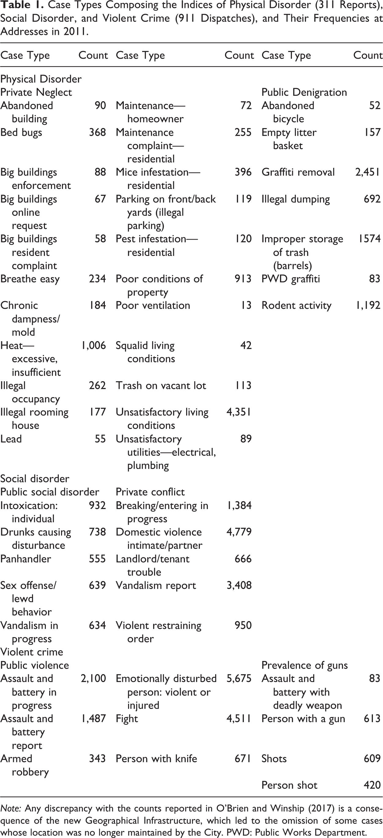
Note: Any discrepancy with the counts reported in O’Brien and Winship (2017) is a consequence of the new Geographical Infrastructure, which led to the omission of some cases whose location was no longer maintained by the City. PWD: Public Works Department.
Units of Analysis
The City of Boston’s street and address management system and tax assessor track all properties (i.e., the smallest ownable unit) and land parcels (i.e., geographically bounded lots that contain one or more properties). Together, these form the basis of the Boston Area Research Initiative’s Geographical Infrastructure for Boston (GI; O’Brien and Gomory 2017), which then maps them both to U.S. Census TIGER line street segments (i.e., the undivided length of street between two intersections or an intersection and a dead end) and nests them within census blocks, block groups, and tracts, as well as other local administrative geographies. Because 311 and 911 requests do not reliably specify the individual property of interest within a land parcel (e.g., condominiums in a building), here we use land parcels as the fundamental unit of analysis and an approximation of the colloquial “address.” The City maintains its own list of land parcels, but the GI condenses this list slightly by combining distinct land parcels with the same postal address that are sufficiently close to each other to be impossible to differentiate in a 311 or 911 report. For our purposes here, this results in a final, three-level database of 98,355 land parcels (from hereon referred to as addresses) situated on 13,048 street segments within 178 census tracts. 8 This nested structure forms the basis for analyses of the distribution of crime and disorder of units within the next highest level of organization (e.g., the addresses on a street). 9 It is important to note that the GI covers all addresses acknowledged by the City, regardless of the presence of a building (e.g., the land use code “Residential Lot” reflects an empty space zoned for residential). Thus, 311 and 911 reports can be attributed to addresses with and without buildings, meaning that the analysis neither omits events at locations without buildings nor incorrectly attributes them to addresses with buildings.
The GI also provides information on urban form that may be relevant to the expected level of crime and disorder at a place including land usage for each parcel (e.g., residential and commercial) and an estimate of the number of units (either as a sum of parcels or the number of units identified by the tax assessor [e.g., two-family residential contains two units]); the street’s length, identification as a main street (provided by MassGIS), and nature of land usage (a seven-group typology based on a cluster analysis of the representation of each land use); and the tract’s population, number of households, and type (e.g., residential, downtown, and park). Table 2 reports descriptive statistics for each of these characteristics.
Characteristics of Addresses, Streets, and Tracts in Boston.
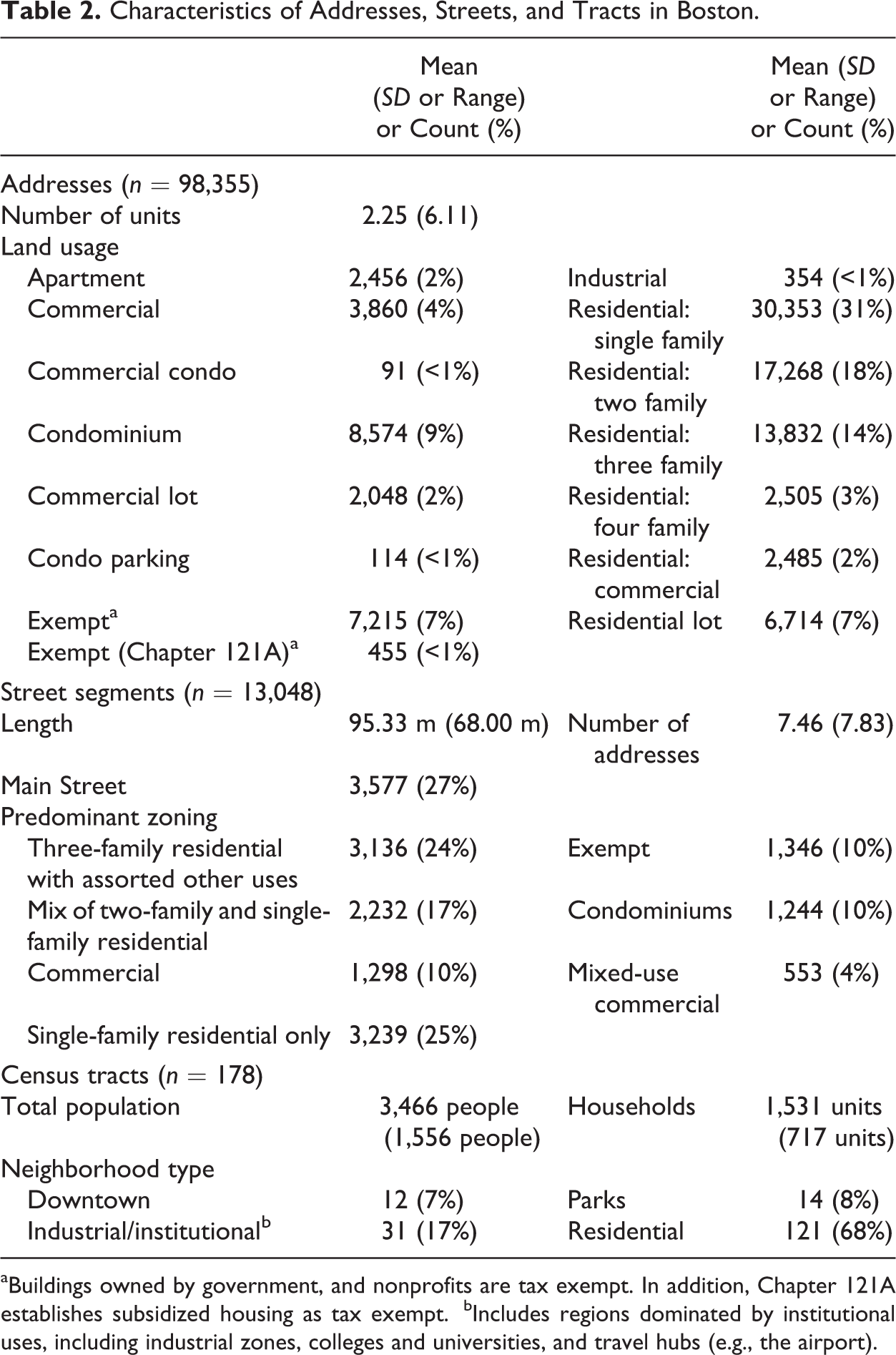
aBuildings owned by government, and nonprofits are tax exempt. In addition, Chapter 121A establishes subsidized housing as tax exempt.
bIncludes regions dominated by institutional uses, including industrial zones, colleges and universities, and travel hubs (e.g., the airport).
Analysis
The main analysis centers on the calculation of Gini coefficients, following the classical equation:

where each member i of a population of n units has a value yi (e.g., addresses with a quantity of gun-related crime reports). When there are fewer events than units (i.e.,

These calculations are conducted in R using the reldist package’s Gini command (Handcock 2016) in conjunction with custom functions. For what will be referred to as global analyses of distribution, the Gini coefficient (i.e., G or G’, as appropriate) is calculated for all units across the city at a given level of geographic organization. For what will be referred to as nested analyses, Gini coefficients are calculated for each “nest” and the central tendency and distribution of the separate Gini coefficients for a given geographic scale is then used to evaluate concentrations at the lower geographic scale. For example, to examine concentrations of crime and disorder at addresses, the nested analyses calculated the Gini coefficient separately for the distribution of events within each of the 13,047 streets with one or more addresses.
Simulations were run in order to evaluate whether Gini coefficients indicate levels of concentration above and beyond what would be expected, given the number of events and units. For each calculated Gini coefficient, the rpois function in R was used to generate 10,000 random Poisson distributions with the same number of events and units. The average of these 10,000 simulated Gini coefficient was used as the point of comparison. For global analyses of all units at a geographical level, this comprised a single simulated expected Gini coefficient. For nested analyses, this comprised a simulated expected Gini coefficient for all higher-level units. For example, the expected Gini coefficient was simulated separately for all 13,047 streets, based on the number of addresses and events associated with each. These were then analyzed in aggregate, paralleling the analysis of the actual Gini coefficients.
The syntax used for these methodologies is available on the Boston Area Research Initiative’s GitHub page (https://github.com/BARIBoston/Gini-Paper).
Results
Descriptive Statistics and Global Analyses of Concentration
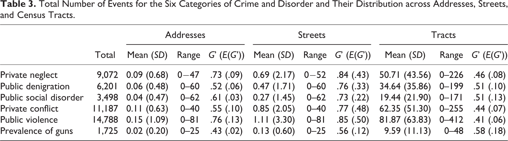
All six forms of disorder and crime were rare events relative to the number of addresses and streets (see Table 3). Even the most common category, public violence, featured one event per seven addresses (M = 0.15) and was the only one with more events than streets (M = 1.27). Others were particularly rare, with the prevalence of guns featuring one event per 50 addresses (M = 0.02). Nonetheless, ranges were quite high (maxima = 25–81 events at an address) and the standard deviations of counts per address and street were universally greater than the corresponding means. This latter point reflects a strong skew, violating the Poisson distribution. This provides preliminary evidence that crime and disorder do in fact concentrate at particular addresses and streets more than would be expected if they were randomly distributed across locations. The story was less extreme for tracts, with the number of events per tract ranging from 9.59 to 81.87 across categories. Corresponding standard deviations were nearer to these values, more in keeping with a true Poisson distribution.
Total Number of Events for the Six Categories of Crime and Disorder and Their Distribution across Addresses, Streets, and Census Tracts.
Gini Coefficients Quantifying the Equality of the Distribution of Crime and Disorder across Addresses on Streets, Streets in Tracts, and Tracts in the City Compared to Expected Values, Both Ignoring and Accounting for Aspects of Urban Form.
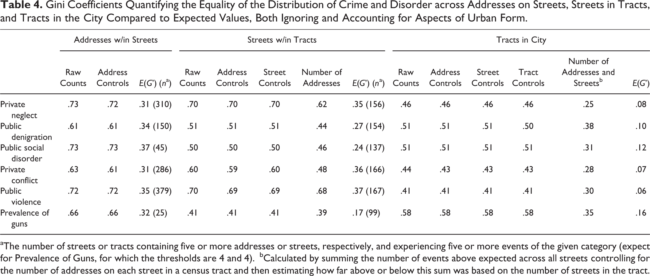
aThe number of streets or tracts containing five or more addresses or streets, respectively, and experiencing five or more events of the given category (expect for Prevalence of Guns, for which the thresholds are 4 and 4).
bCalculated by summing the number of events above expected across all streets controlling for the number of addresses on each street in a census tract and then estimating how far above or below this sum was based on the number of streets in the tract.
When estimating global Gini coefficients, it was necessary to use the modified G’ for all six categories for addresses, and for streets for all categories apart from public violence. 10 Gini coefficients indicated that, when considering the city as a whole, concentrations for all types of crime and disorder were highest at the street level (G’s = .56–.85), then at the address level (G’s = .43–.76), and lowest at the tract level (Gs = .41–.51). For point of comparison, the simulated Ginis (see Methods) indicated that the expected level of concentration was far higher for streets (E(G’)s = .12–.50) than for addresses (E(G’)s = .02–.13) or tracts (E(G’)s = .06–.18). From this perspective, one might argue that addresses have the most notable concentrations relative to statistical expectations. 11 Nonetheless, the interpretation is ambiguous, not to mention that concentrations at one level are partially attributable to those below it when analyzing the data in this way.
Nested Analyses of Concentration
In order to disentangle concentrations of crime and disorder across levels, we can calculate Gini coefficients that nest the units of one level in the containing unit of the next highest geographic level. For example, given the number of gun-related events in a tract, to what extent were they concentrated at certain streets in the tract more than others? This permits an examination of the level of concentration at addresses or streets independent of an existing concentration at a higher level of geography. This technique will generate a Gini coefficient for every street (i.e., the unequal distribution of crimes across the addresses of that street) and tract (i.e., the unequal distribution of crimes across the streets of that tract). We can then compare the typical level of concentration across levels. To avoid uninterpretable outliers, we only calculate Gini coefficients for streets and tracts that have five or more events of a given type of crime or disorder and five or more lower-level units (i.e., addresses or streets, respectively; except in the case of prevalence of guns, whose rarity require a threshold of four events and units to permit sufficient variation for analysis). Note that this does not mean that we omit lower-level units that have fewer than five events when calculating Gini coefficients as that would provide an incomplete view of inequality.
The analysis of nested Gini coefficients occurred in two steps. First, Gini coefficients based on raw counts of events were calculated. Second, they were recalculated using estimates of the number of events above expected for each unit based on the aspects of urban form. For each stage, it was necessary to calculate a “typical” level of concentration for addresses in streets and streets in tracts. Gini coefficients are sensitive to the number of units and events distributed across them, especially when one or the other is a small quantity; concentrations are likely to be higher with a greater volume of events and lower with a greater number of units to spread the events across. In order to fairly compare across levels, we ran regressions using those two variables to predict Gini coefficients. All values reported from hereon will reflect the estimate for five events and five lower-level units. 12 These regressions are reported in the Appendix. Gini coefficients discussed in the following subsections are reported in Table 4.
Distribution of Raw Counts
The nested Gini coefficients differed from the global Gini coefficients in a few ways. Most notably, whereas crime concentrated across the addresses of a given street about equally if not more highly than across all addresses in the city (G’s = .61–.73; equal to or higher than the global analysis for five of six categories), streets tended to show less concentration when nested in tracts, with Gini coefficients dropping by as much as a third (G’s = .41–.70; lower than the global analysis for all categories). This suggests that the high concentration of crime and disorder at street segments across the city is partially attributable to variations across census tracts. In contrast, variations at higher geographic scales were not responsible for the concentrations seen at addresses. Further, events were universally more concentrated across the addresses of a street than the streets of a tract, though these two values were more comparable for some categories (e.g., private neglect and public violence) than others (e.g., public social disorder and prevalence of guns). Again, all Gini coefficients were far higher than those expected for a Poisson distribution of comparable number of events and units (addresses: E(G’)s = .31–.37; streets: E(G’)s = .17–.36). 13
Because tracts were not nested, we compare the global assessments to the other levels. Notably, the lowered Gini coefficients for streets when nested were comparable to tract-level concentrations for a number of measures, including public denigration and public social disorder; most notably, prevalence of guns was much more concentrated for tracts than streets (.58 vs. .41).
Distribution of Events Above Expected
The initial analysis of nested Gini coefficients separated concentrations at one level from the variations at higher levels of geographic organization but did not attend to inherent differences in the distribution of events based on urban form. It is possible that some portion of these concentrations is a consequence of similar types of properties being clustered in space. Here, we use multilevel models to calculate the expected number of events of a given type of disorder or crime for each address in the city relative to addresses on the same street, based on the number of parcels it contains and its land use (see Appendix for full details). The result is a count of events above expected. 14 We can then do the same for street- and tract-level characteristics that are predictive of the number of events at the typical address therein. We only analyze the influence of these characteristics at the geographic level of the controls and above because they would be irrelevant at lower levels of analysis. For example, a parameter estimate at the street level will have the same effect on estimated levels of crime or disorder for all addresses on a given street. This would leave the relative concentration of crime or disorder across those addresses unaltered, meaning there is no need to recalculate the Gini coefficients after accounting for street-level factors. The same logic is true for tract-level characteristics and the Gini coefficients for addresses and streets therein. The analysis then takes account of the number of addresses on each street and streets in each tract, acknowledging the possibility that these higher-order geographies might see concentrations based in part on the uneven distribution of locations where crime and disorder might occur.
Controlling for address characteristics had little, if any, impact on the Gini coefficients at all three levels (addresses: ▵G’s = .00–.01; streets: ▵G’s = .00–.01; tracts: all ▵G’s = .00). The same was true for controlling for street characteristics (streets and tracts: all ▵G’s = .00) and tract characteristics (tracts: ▵G’s = .00–.01). Controlling for the number of addresses on a street and number of streets in a tract, however, lowered the estimated concentration of crime and disorder across the streets of a tract markedly, with Gini coefficients dropping by as much as 20 percent (▵G’s = .01–.12). Even more pronounced, inequality across tracts was cut nearly in half once the number of streets in a tract was taken into account (▵G’s = .11–.23). In sum, these adjustments for the physical composition and organization of the city left address-level concentrations largely intact (G’s ≈ .6–.7) while diminishing concentrations at the street (G’s ≈ .4–.5, with two outliers ≈ .6–.7) and tract levels (G’s ≈ .2–.3 with one value ≈ .4).
Discussion
The results bring new clarity to an empirical debate that has become prominent in recent years: Which geographic level is the most important to the distribution of crime and disorder across a city, or, as some have quipped, “where is the action?” The analysis here made this question tractable by using Gini coefficients in conjunction with three techniques. First, it used the logic of nesting to disentangle concentrations at one geographic level (e.g., addresses) from existing concentrations at higher levels (e.g., streets). Second, it used a modified Gini coefficient that could account for situations in which the units outnumber the events that are distributed across them (Bernasco and Steenbeek 2017). Third, it controlled for aspects of urban form whose own clustering might drive concentrations of crime, like land use and the density of locations where crime and disorder might occur. After accounting for these conditions and factors, concentrations were consistently greatest across addresses, then streets, and lowest for tracts. The action, then, is “everywhere” but becomes increasingly apparent as one zooms in to more and more localized spatial scales. This verified in a general sense the illustrative example in Figure 1, wherein a high-disorder tract has a handful of hotspot streets, one of which is predominated by a single problem property.
Strictly speaking, the finding that concentrations are greater at lower spatial scales is not all that different from previous studies. The few comparisons of streets and neighborhoods (Boessen and Hipp 2015; Schnell et al. 2017; Steenbeek and Weisburd 2016), addresses and neighborhoods (Tseloni 2006), and the one comparison of all three levels (O’Brien and Winship 2017) have observed the same basic relationship. That said, the more comprehensive methodological approach taken here tempered the dramatic differences in concentration observed through multilevel models, which are vulnerable to the abundance of zeroes at lower levels of aggregation. As importantly, we saw how the various considerations of the analysis impacted estimates of concentration. Three such results are worth noting. First, Gini estimates at the street level dropped by ∼20 percent when streets were nested within tracts, but the same effect was not seen for addresses. In some cases, the nested analysis increased the Gini estimates for addresses. This would indicate that a substantial proportion of the concentration of crime at streets is attributable to variations in crime between tracts. Put another way, the distribution of crime across the streets of a tract was more equitable than across all the streets of the city. In contrast, concentrations of crime and disorder at addresses were especially prominent at the local level, possibly because there are many problem properties across the city, but the typical hotspot street segment is dominated by a single such property. Second, controlling for the number of locations in a geography (e.g., addresses on a street) markedly lowered Gini coefficients, especially for tracts, implying that some places have more crime and disorder simply by virtue of having more places where such events can occur. This should not be an entirely surprising finding, but it highlights the fact that this consideration has so rarely been addressed in the criminology of place literature.
The third finding of interest was in fact the lack of an effect. Controlling for land use at each of the three levels had negligible impact on all estimates of concentration of crime and disorder. Even though there is considerable evidence that such characteristics can influence the routine activities and therefore crime and disorder at a place (Bichler et al. 2013; Bowers and Johnson 2005; Eck 1994; Johnson 2008; Johnson et al. 2007; Smith et al. 2000), this is consistent with the argument that only a handful of locations within a particular type (e.g., bar or pub) are chronically problematic (Eck, Clarke, and Guerette 2007). Instead, there are patterns and processes associated with specific places across the city, independent of their land use, that underlie the emergence and persistence of problem properties, hotspot streets, and high-risk neighborhoods. For example, in his ethnography of drug dealers in Chicago, St. Jean (2007) found that certain types of land use do provide ecological advantages for crime but that does not mean that all locations with an advantageous land use will become havens for crime. He details a particular street corner that was a hub for drug sales, in part because of the presence of a bus stop, which provided sufficient activity to distract would-be observers. In addition to the bus stop, the corner had numerous other characteristics—not least of which is the historical recognition as a place where one can go to buy or sell drugs—that sustain its status as a hotspot for drug dealing. Although the bus stop may contribute to this situation, the full story requires a specific confluence of physical characteristics and social habitus that is rather rare.
Before discussing the implications of these findings for theory, research, and practice, it is important to acknowledge a few limitations of the work. First, the analysis is of a single city and will need to be joined by replications in other locales, especially of different sizes or in other countries. Because Gini coefficients are absolute measures, they facilitate the pursuit and implementation of such a research agenda. Second, while the advent of high-quality, digital administrative records has been a recent boon to criminology of place and to urban science more generally, they have their weaknesses as a resource for research (Boyd and Crawford 2012; Lazer et al. 2009, 2014; O’Brien et al. 2015). Most importantly, they are subject to the biases of the data generation mechanism, in this case, the decision of constituents to report events. For example, Klinger and Bridges (1997) found evidence of both erroneous reports (i.e., false positives) and unreported crimes (i.e. false negatives) in constituent calls for service, resulting in a moderate skew in cross-neighborhood crime estimates. More recently, O’Brien et al. (2015) identified differences in “custodianship” that led some neighborhoods to be more likely to report deterioration in the public domain than others; this skew was weaker, however, for reports regarding the deterioration and misuse of private property. In contrast, Hibdon, Telep, and Groff (2017) provide reason to believe that these concerns regarding skew in absolute counts might have a limited impact on generalized analyses of concentration. They found that two service request systems in Seattle, WA, identified different hotspots for drug activity but still described the same overall pattern of concentrations. Third, the study uses census tracts as the highest geographical scale analyzed, though they are known to be loose approximations of “true” neighborhoods at best. There has also been a critique in recent years of whether fixed borders between regions of the city are meaningful at all (Hipp and Boessen 2013). It may be that better specified borders or the adoption of a more flexible approach to defining neighborhoods would provide more precise findings, most likely finding greater concentration of crime across neighborhoods (i.e., assuming that more accurate definitions of neighborhoods result in greater internal homogeneity). That said, the findings here provide a strong first piece of evidence as to the strength of clustering at the scale of census tracts.
Implications for Theory, Research, and Practice
Much of the discussion of concentrations of crime has centered on which geographical scale or scales matter, and the results here further elucidate the relative concentration of crime and disorder at addresses, streets, and neighborhoods. It is important to reiterate that the nature of the analysis was such that the interpretation refers to distributions within a containing geography. That is, neighborhoods vary in their propensity for crime and disorder, but such events concentrate at hotspot streets within tracts and, to an even greater extent, at problem properties on those streets. These findings reraise the theoretical concern of what such concentrations indicate about the geographical organization of crime and its correlates at each of these geographic scales, while also offering a methodological tool for probing such questions further. Additionally, there are implications for policy that must be considered.
The current results most deviate from current trends in criminology of place in the way they highlight problem properties as featuring the greatest concentration of crime. This has a deep history with multiple sources. Some early theorists argued that the multitude of targets meant that offender impulses would be more important than the characteristics of any given place (e.g., Sutherland 1947). On the other hand, those subscribing to the Chicago School’s model of the city have treated addresses and streets as largely subject to the demographic and social dynamics of a broader neighborhood (e.g., Shaw and McKay [1942] 1969; Sampson, Raudenbush, and Earls 1997). Even as recent work has shifted attention to hotspots, the argument has remained that the street segment has characteristic social dynamics that influence its capacity for criminogenesis, with the implication that this might not be true for individual properties (Weisburd et al. 2012; Taylor 1997). In fact, we see here potential for the very opposite: That addresses have the most consistent criminogenic dynamics of all three geographic scales.
There are a number of tools available for making sense of problem properties, particularly routine activity theory and related theories that reduce crime events into three fundamental components: offenders, targets or victims, and the lack of guardians, managers, or others who might interrupt or discourage crime (Cohen and Felson 1979; Brantingham and Brantingham 1993). The simplest interpretation would be that a given problem property is home to one or more “repeat offenders” (Spelman 1994), meaning the geographic concentration is actually an artifact of individuals who are responsible for a disproportionate level of crime. Alternatively, one or more features of the “backcloth” of an address might lead to the sufficiently regular confluence of offenders, suitable targets, and the absence of effective guardians to result in an elevated level of crime or disorder (Brantingham and Brantingham 1993). These might be architectural in nature, with certain physical features either aiding offenders or undercutting targets or guardians (Newman 1973), or they could be social. For example, landlords who fail to establish a strong management system for their property could in turn create a safe haven for activities that generate disorderly behavior, violence, or other disruptions. Eck (1995) provides an example of this in San Diego where he found that drug dealers tended to operate out of apartment buildings whose landlords owned fewer properties and had more debt, suggesting that their limited resources translated into poor supervision. Similar arguments can be made for nonresidential facilities and the ability of their employees to manage the activities that occur there. The critical point here is that the social dynamics of an individual property might create criminogenic patterns that are independent of the neighborhood or street context.
As future research attempts to better understand the dynamics of addresses, it should not lose sight of the higher levels of geographic organization. Most obviously, this is because we still see concentrations of crime and disorder at streets and across neighborhoods. This would suggest that each of the three levels of geographic organization shapes the distribution of offenders, victims, and guardians or managers. For example, an extensive body of work has examined how a community’s capacity for informal social control is critical to limiting crime locally (e.g., Bellair 2000; Bursik and Grasmick 1993; Carr 2005; Shaw and McKay [1942] 1969; Sampson and Groves 1989; Sampson et al. 1997; Steenbeek and Hipp 2011). Work on hotspot streets has recently trended in this direction, including new evidence that street blocks have their own characteristic level of collective efficacy that is involved in shaping crime rates more locally (Weisburd et al. 2017). It would be important to understand the extent to which such processes are responsible not only for the distribution of crimes at the given geographic scale but also at the units within it. For example, is a property with an absentee landlord more likely to become problematic on a street or in a neighborhood with lower income or collective efficacy? Such questions would advance beyond a paradigm that simply compares concentrations of crime at different geographic scales and considers how their characteristics interact with each other (also see Boessen and Hipp 2015).
A second important question is the extent to which various factors at localized scales explain away concentrations at higher ones. To illustrate, the finding that collective efficacy operates at the street level begs the question of whether a neighborhood’s measured collective efficacy really matters for its crime rate, or if, instead, both are just an aggregation of street-level processes. The methodology presented here could be useful for probing these sorts of questions. Land uses and numbers of locations were entered into multilevel models as control factors before calculating Gini coefficients, allowing us to observe clustering at various geographic levels independent of these aspects of urban form. The same technique might be utilized for any covariate that is predictive of crime rates at a given geographic scale. Just as we saw that accounting for numbers of locations diminished Gini coefficients for streets and neighborhoods, we may find that other features of properties or streets account for some portion of clustering at higher levels of aggregation.
Last, it is important to consider what guidance the results here provide for practice. Although they hint at the potential value of microgeographical interventions, like “problem properties task forces” (City of Boston 2011; LISC 2015; Minneapolis 2015), this interpretation is not yet entirely merited. This is because the locus of crime and the locus of causality need not be the same thing. As just discussed, even if crime is more strongly concentrated at addresses, it is possible that the social dynamics of a neighborhood or street are responsible for creating a criminogenic setting within which that problem property can emerge (Weisburd et al. 2012). Thus, it is still feasible that interventions that target problem properties will merely displace crime to other addresses on a street or in a neighborhood. With this in mind, the current study helps to answer a classical question on the distribution of crime across a city, but its greater value is in highlighting the need to answer how such distributions in fact arise and can be addressed by policymakers and practitioners.
Footnotes
Appendix
Complete Parameter Estimates from Multilevel Models Predicting Counts of Reports of Crime and Disorder Based on Characteristics of the Address, Street, and Census Tract.

| Private Neglect | Public Denigration | Public Social Disorder | Private Conflict | Public Violence | Prevalence of Guns | |||||||
|---|---|---|---|---|---|---|---|---|---|---|---|---|
| β (Standard Error) | Odds Ratio | β (Standard Error) | Odds Ratio | β (Standard Error) | Odds Ratio | β (Standard Error) | Odds Ratio | β (Standard Error) | Odds Ratio | β (Standard Error) | Odds Ratio | |
| Address characteristics | ||||||||||||
| Land usagea | ||||||||||||
| Apartment | 2.82*** (.06) | 16.72 | 1.31*** (.05) | 3.72 | 1.66*** (.07) | 5.28 | 2.21*** (.05) | 9.22 | 2.18*** (.06) | 8.87 | 1.24*** (.06) | 3.43 |
| Commercial | 0.13 (.11) | 1.14 | 1.31*** (.06) | 3.71 | 1.83*** (.06) | 6.23 | 0.77*** (.07) | 2.15 | 1.80*** (.05) | 6.04 | 1.01*** (.07) | 2.74 |
| Commercial condo | −0.34 (.42) | 0.71 | 1.81*** (.14) | 6.10 | 2.18*** (.10) | 8.86 | 1.13*** (.21) | 3.10 | 1.57*** (.13) | 4.79 | 1.14*** (.22) | 3.12 |
| Condominium | 1.58*** (.06) | 4.86 | 0.87*** (.05) | 2.39 | 1.22*** (.06) | 3.38 | 1.29*** (.05) | 3.62 | 0.90*** (.06) | 2.45 | 0.80*** (.06) | 2.23 |
| Commercial lot | −0.79*** (.19) | 0.46 | −0.15 (.11) | 0.86 | −0.96*** (.13) | 0.38 | −1.12*** (.15) | 0.32 | −0.34** (.11) | 0.71 | −1.97*** (.22) | 0.14 |
| Exempt | 0.99*** (.07) | 2.69 | 0.69*** (.06) | 2.00 | 1.28*** (.06) | 3.60 | .69*** (.06) | 2.00 | 1.74*** (.05) | 5.72 | 0.56*** (.06) | 1.75 |
| Exempt (121A) | 2.24*** (.13) | 9.44 | 0.58*** (.14) | 1.78 | 1.79*** (.12) | 5.99 | 1.94*** (.10) | 6.97 | 1.81*** (.10) | 6.10 | 1.53*** (.11) | 4.63 |
| Industrial | 0.41 (.30) | 1.50 | 1.41*** (.13) | 4.11 | 0.10 (.19) | 1.10 | −0.14 (.22) | 0.87 | 0.49** (.17) | 1.64 | 0.72** (.20) | 2.06 |
| Residential: two family | 1.16*** (.05) | 3.19 | 0.33*** (.05) | 1.39 | 0.47*** (.06) | 1.60 | 0.73*** (.04) | 2.08 | 0.38*** (.05) | 1.47 | 0.35*** (.05) | 1.42 |
| Residential: three family | 1.79*** (.05) | 6.00 | 0.73*** (.05) | 2.08 | 0.70*** (.06) | 2.00 | 1.24*** (.04) | 3.46 | 0.94*** (.05) | 2.57 | 0.60*** (.05) | 1.82 |
| Residential: four family | 2.41*** (.06) | 11.18 | 1.03*** (.05) | 2.81 | 1.13*** (.08) | 3.08 | 1.77*** (.06) | 5.85 | 1.36*** (.06) | 3.90 | 0.93*** (.07) | 2.53 |
| Residential commercial | 2.12*** (.07) | 8.33 | 1.33*** (.06) | 3.78 | 1.41*** (.06) | 4.08 | 1.72*** (.06) | 5.58 | 1.78*** (.06) | 5.94 | 1.25*** (.07) | 3.48 |
| Residential lot | −0.24* (.09) | 0.79 | −1.08*** (.11) | 0.34 | −3.04*** (.33) | 0.05 | −2.13*** (.16) | 0.12 | −2.05** (.17) | 0.13 | −1.60*** (.11) | 0.20 |
| Number of units | 0.017*** (.001) | 1.02 | 0.009*** (.001) | 1.01 | 0.008*** (.001) | 1.01 | 0.012*** (.001) | 1.01 | 0.015*** (.001) | 1.01 | 0.016*** (.001) | 1.02 |
| Street characteristics | ||||||||||||
| Lengthb | 0.14** (.04) | 1.15 | 0.01 (.04) | 1.01 | 0.15* (.06) | 1.17 | 0.23*** (.03) | 1.27 | 0.29*** (.03) | 1.34 | 0.31*** (.07) | 1.36 |
| Number of parcels | −0.02*** (.003) | 0.98 | −0.01*** (.003) | 0.99 | −0.03*** (.005) | 0.97 | −0.03*** (.003) | 0.97 | −.03*** (.003) | 0.97 | −.04*** (.007) | 0.97 |
| Main streetc | 0.31*** (.05) | 1.36 | 0.27*** (.05) | 1.31 | 0.74*** (.07) | 2.10 | 0.25*** (.04) | 1.28 | 0.50*** (.04) | 1.65 | 0.54*** (.09) | 1.72 |
| Land Usaged | ||||||||||||
| Three family mixed | 0.31*** (.08) | 1.36 | 0.35*** (.08) | 1.42 | 0.60*** (.12) | 1.82 | 0.24*** (.06) | 1.28 | 0.51*** (.07) | 1.67 | 0.96*** (.14) | 2.61 |
| Two family w/ single family | 0.17* (.08) | 1.18 | 0.14 (.08) | 1.15 | 0.24 (.12) | 1.27 | 0.11 (.06) | 1.11 | 0.40*** (.07) | 1.49 | 0.29* (.15) | 1.34 |
| Pure commercial | 0.22 (.13) | 1.25 | 0.45*** (.11) | 1.56 | 1.25*** (.14) | 3.48 | 0.65*** (.08) | 1.92 | 0.64*** (.09) | 1.90 | 1.12*** (.19) | 3.07 |
| Exempt | 0.23 (.12) | 1.26 | 0.04 (.11) | 1.04 | 0.55*** (.15) | 1.73 | 0.41*** (.08) | 1.50 | 0.12 (.09) | 1.13 | 1.12*** (.18) | 3.06 |
| Condominiums | 0.09 (.10) | 1.09 | 0.53*** (.09) | 1.71 | 0.24 (.14) | 1.28 | −0.11 (.07) | 0.89 | 0.14 (.09) | 1.15 | −0.12 (.20) | 0.88 |
| Mixed commercial | 0.50*** (.13) | 1.65 | 0.63*** (.12) | 1.87 | 1.25*** (.16) | 3.49 | 0.31** (.09) | 1.36 | 0.66*** (.10) | 1.94 | 0.95*** (.21) | 2.60 |
| Tract characteristics | ||||||||||||
| Total population (1,000s) | 0.21*** (.06) | 1.24 | −0.21** (.06) | 0.81 | 0.02 (.06) | 1.02 | 0.19*** (.05) | 1.21 | 0.12* (.05) | 1.13 | 0.36** (.10) | 1.43 |
| Total households (100s) | −0.03* (.01) | 0.97 | 0.06*** (.01) | 1.06 | 0.01 (.01) | 1.01 | −0.03** (.01) | 0.97 | −0.01 (.01) | 0.99 | −0.08** (.02) | 0.92 |
| Neighborhood typee | ||||||||||||
| Downtown | −0.81*** (.22) | 0.45 | 0.48* (.22) | 1.62 | 0.26 (.22) | 1.30 | −0.18 (.18) | 0.83 | −0.04 (.19) | 0.96 | −0.65 (.39) | 0.52 |
| Institutional | −0.10 (.13) | 0.91 | 0.46** (.15) | 1.58 | 0.22 (.15) | 1.25 | −0.12 (.12) | 0.89 | −0.08 (.12) | 0.92 | −0.66** (.24) | 0.52 |
| Park | 0.04 (.21) | 1.05 | −0.33 (.25) | 0.72 | −0.25 (.25) | 0.78 | 0.15 (.18) | 1.16 | −0.13 (.19) | 0.87 | −0.28 (.38) | 0.76 |
| N (roads/tracts) | 97,287 (13,045/178) | 97,287 (13,045/178) | 97,287 (13,045/178) | 97,287 (13,045/178) | 97,287 (13,045/178) | 97,287 (13,045/178) | ||||||
Note: n = 98,287 addresses nested in 13,045 street segments in 178 census tracts for which sufficient information was available to run the models.
aA series of dichotomous variables reflecting an address’ land usage, with residential: single family acting as the reference group. Parameters were not estimated for two land uses with very few addresses (agricultural and condo parking).
b100s of meters.
cA dichotomous variable with “1” equal to variable name.
dA series of dichotomous variables reflecting a street’s predominant land usage, based on a cluster analysis of land use types. Single-family residential is the reference group.
eA series of dichotomous variables reflecting a tract’s predominant usage, with residential acting as the reference group.
*p < .05. **p < .01. ***p < .001.
Acknowledgments
The author would like to thank the Department of Innovation and Technology, the Mayor’s Office, the Mayor’s Problem Properties Task Force, and the Boston Police Department for data sharing and collaborative assistance and Anthony Braga and members of the Boston Area Research Initiative research team for commenting on earlier drafts.
Declaration of Conflicting Interests
The author(s) declared no potential conflicts of interest with respect to the research, authorship, and/or publication of this article.
Funding
The author(s) disclosed receipt of the following financial support for the research, authorship, and/or publication of this article: This study has been supported by the National Science Foundation (Grant # SES-1637124).