Ditching the norm: Using alternative distributions for biological data analysis

Introduction

Statistical tests commonly used in biology such as t-tests, analyses of variance, and regressions assume a normal or Gaussian distribution for the data. However, real data are often bounded, skewed, censored, truncated, have outliers, or do not follow a normal distribution for another logical reason. A common response is to switch to non-parametric tests, but these methods replace the measured values by ranks, which loses information. In addition, no conclusions can be drawn about effect sizes (e.g. mean difference between groups), they cannot be used to make predictions, they are highly sensitive to their own set of assumptions and they may alter the hypothesis being tested. ¹

The data of any experiment or observational study can be considered as arising from an unidentified statistical distribution. Nature need not conform to a distribution invented by humans, but it is convenient to represent the data as having been generated from such a distribution to enable parametric statistical inference. There is no good reason to use a normal distribution for all analyses when many more distributions are available, and selecting an appropriate distribution is an integral part of the data analysis process.

Suppose we run an experiment in which 20 animals are randomly assigned to either a control ( C ) or drug ( D ) condition with 10 animals in each group. We can represent this with the following pair of equations, where y is the outcome variable and the subscript i is the animal index. Animals 1 to 10 are controls and animals 11 to 20 receive the drug.

The tilde ( ∼ ) is read as ‘is distributed as’ or ‘is generated from’, and so the control data in the first equation are generated from some unspecified distribution (Dist) with a mean of μ C and a standard deviation of σ . Similarly, the outcome values in the drug group are generated from the same distribution with a different mean of μ D and the same standard deviation σ . There is no C or D subscript on σ , indicating that we are assuming a common within-group standard deviation for the two groups (the homogeneity of variance assumption).

In an actual experiment, we only know the y i values and the experimental group an animal belongs to. Given this information, we need to select the distribution (Dist) that we believe generated the y i values and then estimate all of the parameters ( μ C , μ D , σ ). Finally, we can test whether the mean parameters differ between groups. This is called a parametric analysis because we test or compare parameters from statistical distributions. Therefore, to be able to compare μ C and μ D sensibly, the distribution we select should reasonably describe the y i s. If choosing a distribution seems strange, it is because biologists are usually taught only the normal distribution and are expected to use it for most analyses.

The normal distribution plays another role in statistics: as the sample size increases, the uncertainty in the μ s approximates a normal distribution, even if the y i s follow some other distribution (Central Limit Theorem). This approximation may be poor in some in vivo experiments as sample sizes tend to be small, which leads to inaccurate p-values and confidence intervals when the distribution of the data is far from normal.

Four alternative distributions

In the following section, we describe the Poisson, Student-t, Gamma and Beta distributions and the types of data they are suitable for. They can be used with any experimental design (multiple groups, multiple factors, continuous variables, nested data) and form a class of models called generalised linear models. An example data set for each distribution is shown in Figure 1. Table 1 shows the results of analysing the data using the appropriate distribution (‘Best’), a normal distribution and a non-parametric Wilcoxon test.

OPEN IN VIEWER

Figure 1.

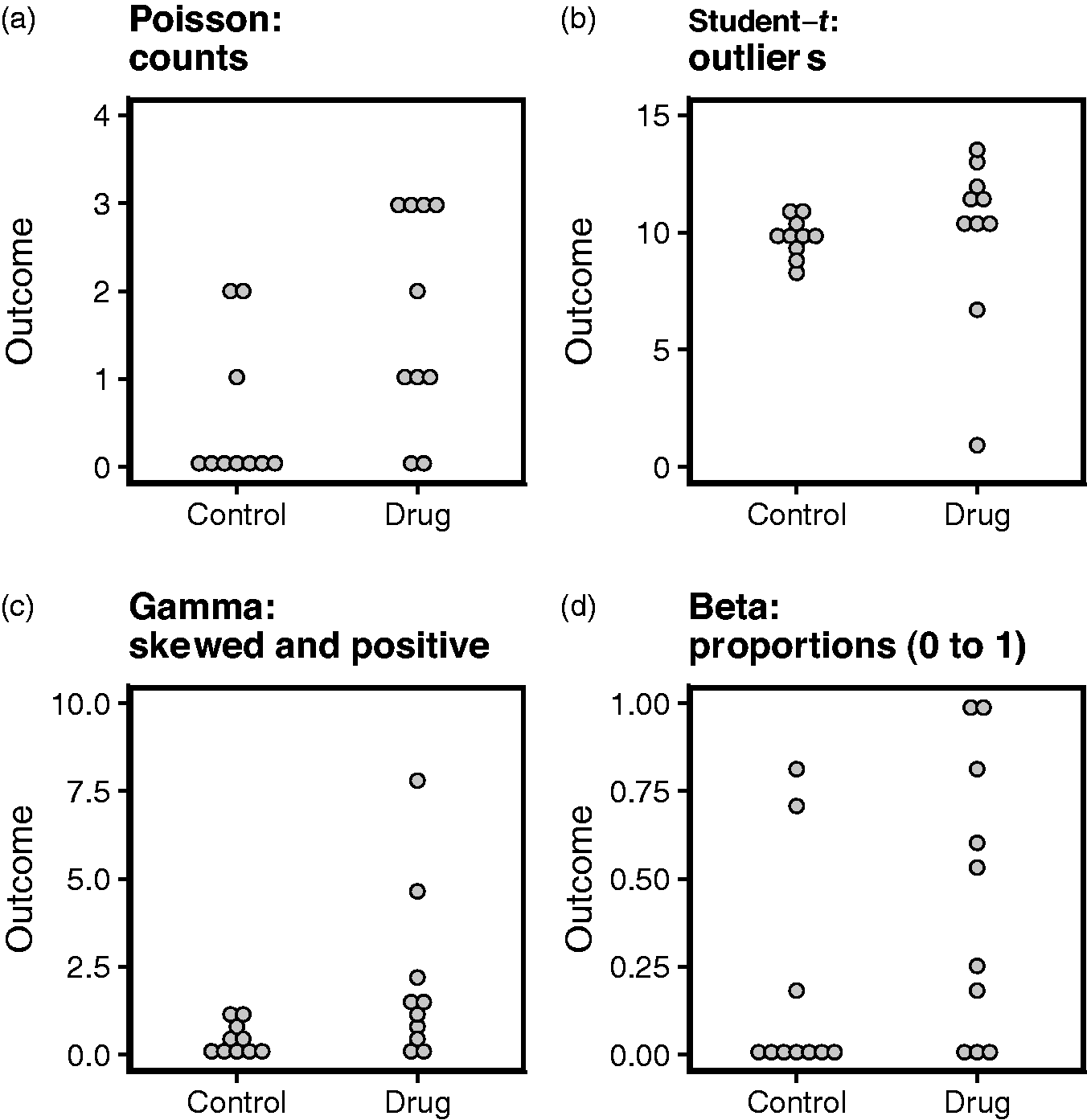
(a) to (d) Four distributions and the type of data they are suitable for.

OPEN IN VIEWER

Table 1.

Analysis summary. p-values for the drug effect and estimates (95% confidence interval (CI)) for the mean difference between groups. The CI width is calculated as the upper minus the lower 95% CI value and measures the precision of the estimate. Residual p is the p-value for testing the normality of the residuals (p < 0.05 means the residuals are not normally distributed). Predictions indicates whether model predictions include impossible (e.g. negative) values. All values are possible with a Student-t distribution, so a model cannot have impossible predictions (N/A). The Normal model analysis for the Gamma-distributed data was performed on log-transformed values.

		Poisson	Student-t	Gamma	Beta
Best	p-value	0.027	0.018	0.011	0.087
	Estimate	1.22	1.32	1.60	0.27
	95% CI	(0.23, 2.22)	(0.34, 2.30)	(0.5, 2.7)	N/A
	CI width	1.99	1.96	2.2	N/A
	Residual p	0.985	0.866	0.900	0.998
	Predictions	OK	N/A	OK	OK
Normal	p-value	0.017	0.870	0.293	0.100
	Estimate	1.20	0.18	0.94	0.27
	95% CI	(0.31, 2.09)	(−2.06, 2.42)	(−0.76, 2.64)	(−0.04, 0.57)
	CI width	1.78	4.48	3.4	0.61
	Residual p	0.008	<0.001	0.023	0.008
	Predictions	Impossible	N/A	OK	Impossible
Wilcoxon	p-value	0.025	0.075	0.089	0.089

Count data are non-negative integers (0, 1, 2, 3, etc.) and therefore are bounded below by zero. The data may contain only a few discrete values, making a normal distribution inappropriate. It is only when the data are close to zero that the lower bound and discreteness make the normal approximation less accurate. If the counts are large and far from zero, they can often be approximated with a normal distribution. Furthermore, the variance of count data typically increases with the mean, violating the homogeneity of variance assumption. Figure 1(a) shows an example of such data, which could be the number of tumours each animal has, or the number of marbles buried by each animal in the marble burying test. The data in this example contain only four unique values (0–3), and an alternative distribution for such data is the Poisson. The Poisson distribution has a single parameter for the mean, and no separate parameter for the variance, which is assumed proportional to the mean (the Negative Binomial distribution is also appropriate for count data and has a parameter for the variance). Analysis of this data using a Poisson distribution (‘Best’ in Table 1), normal (t-test) or a non-parametric Wilcoxon test gives similar p-values and overall conclusions. But there is more to an analysis than p-values – when using a normal distribution predictions include negative values, which are impossible since the data are counts and must be ≥ 0 . Furthermore, the residuals (the difference between the actual and predicted values) should be normally distributed, but this is not the case for the normal model, indicating that the normal approximation is poor, and the p-values may be unreliable.

Outliers in data are common. Figure 1(b) shows one or two outliers in the drug group, which also causes the variance to be larger than the control group. Without these outliers, the drug appears to have a higher average value. Assume these outlying points are reproducible features of such an experiment and not a one-off event particular to this experiment. It is better to use a distribution that allows for outliers instead of removing them using arbitrary criteria. In such cases, a Student-t distribution can be used. Student-t distributions are generalisations of normal distributions with a third parameter that can either be fixed or estimated from the data and which accounts for the outliers. Both the standard t-test (which assumes the data are normally distributed) and Wilcoxon test give p-values greater than 0.05, but modelling the data as arising from a t-distribution gives p = 0.018, so the result would differ depending on the analysis (Table 1). The normal distribution performed especially bad in this analysis with a different estimated effect size, a much wider 95% confidence interval (CI) width (less precision) and non-normal residuals.

Many outcomes are bounded by zero, positively skewed, and often cover several orders of magnitude (Figure 1(c)). These include time-to-event data, such as time to complete a maze or survival time, as well as concentrations of genes, proteins or metabolites. Furthermore, the variances of these data tend to be higher in groups with higher means. A log-transformation is often used to normalise the data and equalise the variances, which are then analysed using a normal distribution. This implicitly assumes the original values are log-normally distributed. Even though log-transforming the data may improve the skewness and unequal variances, it may not be the best transformation. ² Another option is to directly model the data as log-normally distributed. The main advantage is that we can compare the log-normal distribution with other similar distributions that might better describe the skewness, such as a Gamma or Weibull distribution. The Weibull distribution, for example, is often used for survival analysis. These data were simulated from a Gamma distribution, and Table 1 compares a Gamma model with a normal model on the log-transformed values. Despite log-transforming these data, a normal model has much less power (larger and non-significant p-value), less precision, and still has non-normal residuals. Hence, different conclusions would be reached when using the Gamma model versus a normal model on log-transformed data or a non-parametric test.

Finally, data may be proportions or percentages which lie between zero and one (Figure 1(d); percentages can always be divided by 100 to put them between zero and one). Furthermore, these data are characterised by small variances at the ends of the range and a maximal variance in the middle. Examples include body fat percentage or the proportion of time spent in the target quadrant of the Morris water maze. The Beta distribution is appropriate for this type of data as it is defined for values between zero and one. ³ In cases where the values are in the middle of the range, a normal distribution may be reasonable. Note that the Beta distribution is appropriate for ‘parts of a whole’ data and not for counts such as ‘ x out of n ’; for example, seven errors out of 20 attempts, or 18 positive cells out of 200 (a Binomial distribution is then applicable). As shown in Table 1, all analyses yield a similar p-value, but the predictions for the normal model again include impossible values and the residuals are not normally distributed (95% CIs are not reported as they are not directly comparable to the normal model results).

Across the different data sets the Wilcoxon test often returns similar p-values as the best analysis – illustrating one of the benefits of non-parametric methods. But they cannot be used for more complex analyses, such as adjusting for baseline measurements or body weight, and they provide no estimate of mean differences between groups and the associated uncertainty, and they cannot be used to make predictions.

Summary

Researchers sometimes believe that non-normal data indicate a problem with the data, but it usually reflects a problem with the chosen distribution. An appropriate distribution must be selected as part of an analysis, but how is the distribution determined? Using background knowledge (are the data counts?) and also empirically, by examining residuals and whether data simulated from the model resemble the observed data. ⁴ The gamlss R package contains these distributions, as well as many others, and the brms R package can be used for Bayesian analyses.^5,6 Both of these packages have distributions for censored, truncated and zero inflated data, which are additional reasons that observed values may deviate from normality. Crawley provides a general introduction to R and how to analyse these types of data using biological examples, ⁷ and see Gelman et al. ⁸ and Westfall and Arias ⁹ for a general introduction to data analysis. These methods are unavailable in GraphPad Prism and Excel, and therefore these products cannot be recommended. However these methods are available in most statistical software such as SPSS, SAS, JMP and Stata, and details can be found in their documentation.