Comparison of high-volume instrument and advanced fiber information systems based on prediction performance of yarn properties using a radial basis function neural network

Abstract

In this study, an artificial neural network (ANN) model is presented in order to predict the tenacity and hairiness of carded cotton yarns. Fiber measurement values generated by using a high-volume instrument (HVI) and an advanced fiber information system (AFIS) were used in the ANN model as input parameters. The radial basis function neural network (RBFNN) was used as ANN structure. The best RBFNN model was determined by analyzing the effect of epochs and the number of neurons on prediction performance. By using this ANN structure, the comparison between the performance of predicting yarn properties from HVIs and from AFISs was carried out. In the study, four different yarn counts (Ne20, Ne24, Ne30, and Ne40) for 10 different blends were applied. Each yarn count was spun at 4.34α_e twist factor. In this study, the model presented a good rate of accuracy for predicting yarn tenacity and hairiness by using HVI and AFIS fiber values. The study showed that there was no significant difference between the accuracy of predicting these yarn properties from HVI fiber measurement results and those from an AFIS by using the RBF. From the results, it was noted that the performance of predicting yarn hairiness was better than that of predicting yarn tenacity. Also, this study could provide researchers with exclusive information on how to select the most appropriate ANN architecture and how to evolve the model for testing.

Keywords

Radial basis function yarn tenacity yarn hairiness artificial neural networks prediction models fiber properties

Introduction

Knowledge of the relationship between performance and characteristic parameters of yarns made from given fibers assists the producers to arrange the technological processes. This will allow a producer to make an informed decision that accounts for the required quality of the yarn at the best price. So, modeling and predicting yarn properties by putting forward the relationship between the fiber and the yarn properties are two of the most remarkable subjects for textile researchers. Many statistical^1–9 and mathematical^9–16 models have been developed to address prediction accuracy and general applicability. Mathematical models are usually based on certain idealized assumptions, so their success potential is mainly limited by the viability of these assumptions. In recent years, neural networks have been shown as efficient alternatives to first principle models due to their ability to describe highly complex and nonlinear problems in many fields of engineering.¹⁷

Artificial neural networks (ANNs) have received much attention recently. Like their biological counterparts, ANNs learn from experience, generalize, and perform abstraction. They have been taught with suitable training sets to perform well in a wide range of applications. An ANN is a network of simple processing elements that can exhibit complex global behaviors, determined by the connections between the processing elements and element parameters. These elements are known as neurons. An artificial neuron is a mathematical function conceived as a simple model of a real (biological) neuron. In an ANN structure, firstly, a set of input connections brings in activations from other neurons; secondly, a processing unit sums the inputs and then applies a nonlinear activation function; finally, an output line transmits the result to other neurons. An ANN is also a nonparametric estimation technique. It does not make any distributional assumptions regarding the underlying variable. Instead, it presents a formula with a set of unknown parameters and lets the optimization routine search for the parameters that are best fitted to produce the desired results.¹⁸ Different learning types of neural networks are used in modeling studies. However, the most common classifications are made as supervised and unsupervised learning networks. A supervised learning network contains pairs of input and output data. There is a selected output dataset for each input dataset. In this type of learning, the key point is that the desired output of the network is known for each input dataset. Hence, the weights of the network can be modified. Supervised neural networks are typically used to solve function approximation, using examples of the function in the form of input-output pairs. In unsupervised learning, the output is not known. The learning is simply carried out by using input data.¹⁹

ANNs consist of a large class of different architectures. However, most research related to predicting yarn properties focuses on the use of multilayered perceptron neural networks (MLPNNs) trained by back-propagation learning algorithms. Numerous applications of MLPNNs in developing models of predicting yarn properties have been reported.^20–33 Zeng et al.²⁰ presented the prediction models of air-jet spun yarn tenacity based on nozzle pressure, nozzle design and spinning speed. They used two techniques, namely, numerical simulation and the ANN model, and compared these models in respect to prediction accuracy. They concluded that the predicted and experimental values of yarn tenacity were relatively similar. Babay et al.²¹ developed a linear regression model and an ANN model to predict cotton yarn hairiness from fiber properties measured by an high-volume instrument (HVI) system. They achieved good prediction accuracy by using the ANN model. Dayik⁸ reported a prediction model of cotton yarn strength from fiber properties measured by an HVI system. Furferi and Gelli²² studied the prediction of strength of different yarn compositions. Majumdar and Majumdar⁹ used a linear multiple regression algorithm, a mathematical model, and an ANN model to predict the breaking elongation of ring-spun cotton yarns from fiber properties measured by an HVI system. They found that the prediction accuracy was best for the ANN model followed by the statistical and mathematical models, respectively. Gharehaghaji et al.²³ researched the prediction performance of ANN and multiple linear regression models for breaking elongation and breaking strength of cotton-covered nylon core yarns. They considered the count of core part, the count of sheath part, and the twist factor as input data and an MLPNN as the ANN structure. They found that the prediction performance of the ANN model was better than that of the linear model. Yadav and Kothari²⁴ presented a prediction study on air-jet textured polyester yarn properties, which included instability, physical bulk, and tenacity. They compared prediction performance of the MLPNN with the regression model based on the response surface design. They concluded that the mean square errors in MLPNN were higher in number than the number of errors that occurred in the response surface design model. Beltran et al.²⁵ predicted yarn neps, unevenness, tenacity, elongation at break, and thin and thick places of worsted yarn by using a MLPNN and a special program named Sirolan Yarnspec. They obtained better prediction accuracy using the MLPNN than with the Sirolan Yarnspec. Ramesh et al.²⁶ studied the prediction of breaking elongation and breaking load of air-jet spun yarn. In the study, blend, yarn count, and front and back nozzle pressures were considered as input data. Ramesh et al. achieved a good prediction performance. Shanbeh et al.²⁷ predicted the breaking strength and mass irregularity of cotton rotor-spun yarns containing cotton fiber recovered from the ginning process. They developed an ANN model by using rotor diameter, rotor speed, naval type, and yarn count as input data. Desai et al.²⁸ developed an ANN model to predict cotton yarn tenacity and unevenness from fiber properties measured with an HVI system. They compared the predicted output data with the actual data using statistical analyses. Ureyen and Gürkan^29,30 compared the ANN and linear regression models for predicting ring-spun yarn hairiness, unevenness, and tensile properties by using ANN model including back-propagation algorithm. Khan et al.³¹ developed an MLPNN model to predict the hairiness of worsted yarns. Cheng and Adams³² predicted yarn strength and presented the relationship between yarn strength and fiber properties by using ANN model including back-propagation algorithm. Mwasiagi et al.³³ tried to predict the elongation of ring-spun yarn from fiber properties. It is obvious from this discussion that the MLP type of neural networks have been used often. However, MLPNNs have some disadvantages, such as slow training speed, local minimal convergence behavior, sensitivity to the randomly selected initial weight values, and difficulty in explicit optimum network configuration.¹⁸ To solve the problems in all mentioned investigations, an radial basis function neural network (RBFNN), which is another ANN architecture, is proposed by many researchers from different engineering fields.¹⁸ An RBFNN has only one hidden unit, while an MLPNN has one or more hidden layers. The output layer of an RBFNN is linear, while the output layer of an MLPNN is nonlinear.¹⁸ These characteristics provide RBFNNs with advantages, such as simple architectures, fast training speeds, near-optimal solutions, and easy optimization of topology.¹⁸ Therefore, an RBFNN has been used extensively in systems modeling and prediction studies for many different engineering applications.^18,34–43

When the aforementioned studies are considered in respect to input and output data, it can be noted that most researchers have concentrated on the prediction of yarn tenacity and elongation from HVI fiber measurements, whereas fewer investigations on predicting yarn properties from AFIS fiber measurements have been conducted.

The focus of this study is to predict the tenacity and hairiness values of carded yarn from HVI and advanced fiber information system (AFIS) fiber measurements by using the RBFNN modeling method and comparing the performance of predicting yarn properties from HVI fiber measurement values with those of AFIS fiber measurement values.

1. Materials and methods

1.1 Materials

In this paper, the tenacity and hairiness of carded yarns that were spun by using 10 different cotton fiber mixes were predicted. The blends are from the Aegean and Urfa areas in Turkey, Greece, and Syria. These countries export cotton fiber to many other countries throughout the world. Therefore, this selection of blends covers a good degree of variety. All blends were spun into yarns on a ring-spinning machine (Rieter G30) at yarn counts of Ne20, Ne24, Ne30, and Ne40 at Abalioglu Yem, Soya and Tekstil Spinning Mill, Denizli, Turkey. Each yarn count was spun at 4.34α_e twist factor. Fiber properties were measured by using HVI and AFIS measurement systems. The tenacity and hairiness of the yarns were measured by using USTER tensorapid and Uster tester 3, respectively. Table 1 presents the properties of the fibers belonging to each blend.³⁸

Table 1.

Fiber properties measured by using HVI and AFIS³⁸ and the dataset for RBFNN modeling

Input data (Fiber properties and yarn count)																Experimental
		HVI measurement results							AFIS measurement results							Output data
Data line	Blend	Y.C.¹	Fine	UHML	Uni.³	Str.⁴	Elong.⁵	S.F.⁶	Y.C.	L(w)	L(w)	SFC(w)	Fine	Mat	Neps	Y.T.⁷	Y.H.⁸
Nr.	type	(Ne)	mic.²	(mm)	%U	(gr/tex)	(%)	(%)	(Ne)	mm	%CV	%	mtex	ratio	Cnt/gr	cN/tex	H
1	B1	20	4.34	30.17	82.22	27.15	6.96	6.95	20	25.77	32.40	7.08	165.44	0.88	118.46	17.61	7.21
2	B2	20	4.22	30.10	83.03	23.75	7.06	7.51	20	25.58	32.89	7.29	162.74	0.87	126.91	17.20	7.35
3	B3	20	4.44	28.86	83.50	27.84	7.09	9.07	20	24.68	33.32	8.96	162.17	0.85	267.25	17.03	7.29
4	B4	20	4.16	30.18	84.94	32.23	7.73	7.07	20	25.76	32.12	7.30	163.30	0.87	114.74	17.71	7.36
5	B5	20	3.94	29.64	82.61	30.77	7.03	8.77	20	24.70	34.49	8.33	151.38	0.86	234.86	19.04	6.86
6	B6	20	4.18	29.73	82.62	30.70	7.01	8.37	20	24.87	34.63	8.44	152.36	0.86	224.15	17.99	7.15
7	B7	20	4.18	28.67	82.97	30.11	7.28	8.73	20	24.51	33.26	8.84	165.57	0.87	209.34	17.09	7.13
8	B8	20	4.27	29.19	82.58	30.75	7.03	8.85	20	24.56	34.58	8.78	155.21	0.87	220.55	18.77	6.79
9	B9	20	4.14	29.59	83.67	31.86	7.79	7.79	20	24.83	33.75	8.99	162.40	0.85	234.23	16.75	7.14
10	B10	20	4.19	29.59	83.80	32.11	7.79	7.76	20	24.83	33.83	9.00	161.50	0.84	217.08	16.55	7.06
11	B1	24	4.34	30.17	82.22	27.15	6.96	6.95	24	25.77	32.40	7.08	165.44	0.88	118.46	17.27	6.83
12	B2	24	4.22	30.10	83.03	23.75	7.06	7.51	24	25.58	32.89	7.29	162.74	0.87	126.91	16.65	6.78
13	B3	24	4.44	28.86	83.50	27.84	7.09	9.07	24	24.68	33.32	8.96	162.17	0.85	267.25	17.17	6.71
14	B4	24	4.16	30.18	84.94	32.23	7.73	7.07	24	25.76	32.12	7.30	163.30	0.87	114.74	16.94	6.87
15	B5	24	3.94	29.64	82.61	30.77	7.03	8.77	24	24.70	34.49	8.33	151.38	0.86	234.86	18.29	6.40
16	B6	24	4.18	29.73	82.62	30.70	7.01	8.37	24	24.87	34.63	8.44	152.36	0.86	224.15	17.99	6.52
17	B7	24	4.18	28.67	82.97	30.11	7.28	8.73	24	24.51	33.26	8.84	165.57	0.87	209.34	17.65	6.48
18	B8	24	4.27	29.19	82.58	30.75	7.03	8.85	24	24.56	34.58	8.78	155.21	0.87	220.55	18.52	6.23
19	B9	24	4.14	29.59	83.67	31.86	7.79	7.79	24	24.83	33.75	8.99	162.40	0.85	234.23	16.50	6.74
20	B10	24	4.19	29.59	83.80	32.11	7.79	7.76	24	24.83	33.83	9.00	161.50	0.84	217.08	16.56	6.66
21	B1	30	4.34	30.17	82.22	27.15	6.96	6.95	30	25.77	32.40	7.08	165.44	0.88	118.46	16.54	6.26
22	B2	30	4.22	30.10	83.03	23.75	7.06	7.51	30	25.58	32.89	7.29	162.74	0.87	126.91	16.81	6.26
23	B3	30	4.44	28.86	83.50	27.84	7.09	9.07	30	24.68	33.32	8.96	162.17	0.85	267.25	16.14	6.96
24	B4	30	4.16	30.18	84.94	32.23	7.73	7.07	30	25.76	32.12	7.30	163.30	0.87	114.74	16.78	6.29
25	B5	30	3.94	29.64	82.61	30.77	7.03	8.77	30	24.70	34.49	8.33	151.38	0.86	234.86	18.57	5.68
26	B6	30	4.18	29.73	82.62	30.70	7.01	8.37	30	24.87	34.63	8.44	152.36	0.86	224.15	17.28	5.96
27	B7	30	4.18	28.67	82.97	30.11	7.28	8.73	30	24.51	33.26	8.84	165.57	0.87	209.34	16.59	5.92
28	B8	30	4.27	29.19	82.58	30.75	7.03	8.85	30	24.56	34.58	8.78	155.21	0.87	220.55	18.05	5.67
29	B9	30	4.14	29.59	83.67	31.86	7.79	7.79	30	24.83	33.75	8.99	162.40	0.85	234.23	16.04	5.91
30	B10	30	4.19	29.59	83.80	32.11	7.79	7.76	30	24.83	33.83	9.00	161.50	0.84	217.08	15.87	5.92
31	B1	40	4.34	30.17	82.22	27.15	6.96	6.95	40	25.77	32.40	7.08	165.44	0.88	118.46	15.56	5.79
32	B2	40	4.22	30.10	83.03	23.75	7.06	7.51	40	25.58	32.89	7.29	162.74	0.87	126.91	15.46	5.27
33	B3	40	4.44	28.86	83.50	27.84	7.09	9.07	40	24.68	33.32	8.96	162.17	0.85	267.25	15.50	6.12
34	B4	40	4.16	30.18	84.94	32.23	7.73	7.07	40	25.76	32.12	7.30	163.30	0.87	114.74	15.63	5.98
35	B5	40	3.94	29.64	82.61	30.77	7.03	8.77	40	24.70	34.49	8.33	151.38	0.86	234.86	17.42	5.15
36	B6	40	4.18	29.73	82.62	30.70	7.01	8.37	40	24.87	34.63	8.44	152.36	0.86	224.15	16.96	5.46
37	B7	40	4.18	28.67	82.97	30.11	7.28	8.73	40	24.51	33.26	8.84	165.57	0.87	209.34	16.35	5.41
38	B8	40	4.27	29.19	82.58	30.75	7.03	8.85	40	24.56	34.58	8.78	155.21	0.87	220.55	17.60	5.16
39	B9	40	4.14	29.59	83.67	31.86	7.79	7.79	40	24.83	33.75	8.99	162.40	0.85	234.23	15.17	5.25
40	B10	40	4.19	29.59	83.80	32.11	7.79	7.76	40	24.83	33.83	9.00	161.50	0.84	217.08	15.74	5.34
	1) Yarn count				3) Uniformity			5) Elongation				7) Yarn tenacity
	2) Microner				4) Strength			6) Short fiber index				8) Yarn hairiness

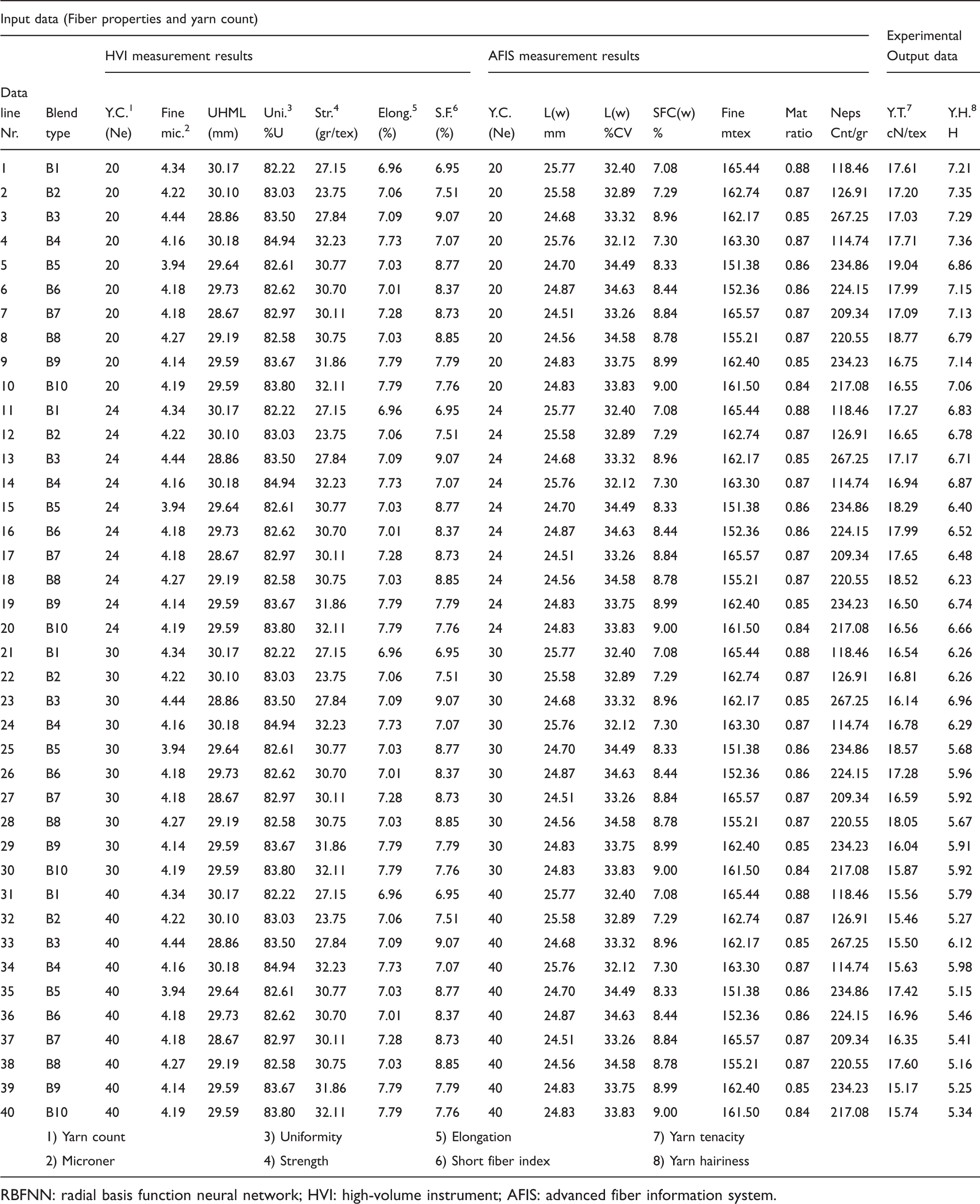
RBFNN: radial basis function neural network; HVI: high-volume instrument; AFIS: advanced fiber information system.

1.2 Method

This section contains two main parts. In the first part, information about the RBFNN is presented. In the second part, the implementation of the RBFNN in this study is explained.

1.2.1 RBFNNs

In this study, RBFNNs are used as the ANN structure. Overall neural network structures, RBFNNs have proven to yield successful results in function approximation type problems.^18,34–43

RBFs were first used to solve multivariable interpolation problems.⁴⁵ RBFNNs could be seen as a sensible alternative to the mentioned attempts to use complex polynomials for function approximation. The schematic diagram of the RBFNN for one output is given in Figure 1.⁴⁵

Figure 1.

Schematic diagram of the radial basis function neural network for one output.⁴⁵

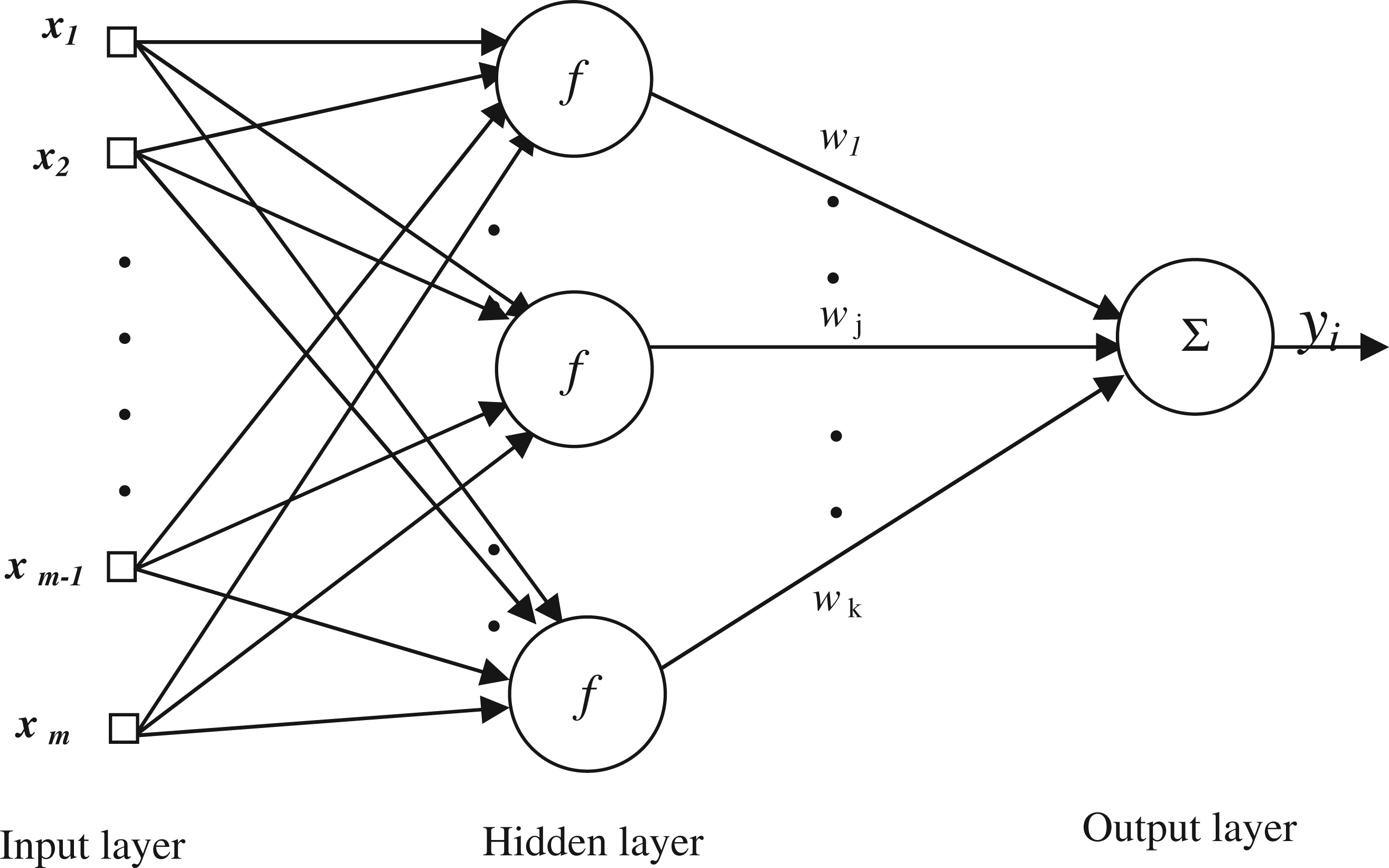
The RBFNN structure contains three layers: the input layer, the hidden layer, and the output layer. The input layer is made up of source nodes that connect the structure to its environment. The hidden layer carries out a nonlinear transformation from the input space to the hidden space. The third layer, the output layer, provides the response of the network to the activation pattern applied to the input layer.⁴⁵ There is only one hidden layer that uses neurons with RBF activation functions. A function is called RBF if its output depends on the distance of the input from a given stored vector. Different functions such as multiquadrics, inverse multiquadrics, and biharmonics could be used as a RBF.³⁹

The commonly used RBFNN function is the Gaussian function. The Gaussian function approaches 0 for large distance, r, values. Thus, even for the input patterns that are different from all teaching patterns, the learning will be still simple to predict. Additionally, the Gaussian function can generate beneficial results without the use of shortcut connections between the input and output layers.⁴⁶ A Gaussian function in which the output of the j ^th hidden unit can be written as^45,46

\begin{matrix} f_{ij} (x) = \exp (- \frac{‖ x_{i} - c_{j} ‖^{2}}{2 σ_{j}^{2}}) i = 1, 2, \dots, m \\ and j = 1, \dots, k \end{matrix}

(1)

where

$f_{ij}$ is the j ^th hidden unit output for the i ^th input data,

σ _i is the width of the RBF at the i ^th hidden unit,

c_i is the center of RBF at the i ^th hidden unit (c_i ∈ ℜ^1×n),

j is index of the number of hidden units.

k is the maximum number of hidden units,

i is index of the number of input data,

n is the number of input variables,

m is the size of dataset, and

$x_{i}$ is the i ^th input data vector ( $x_{i}$ ∈ℜ^1×n)

X = [\begin{matrix} x_{11} & \dots x_{1 n} \\ : & : \\ x_{m 1} & \dots f_{mn} \end{matrix}] \equiv [\begin{matrix} x_{1} \\ : \\ x_{m} \end{matrix}]

(2)

In this case, the distance between the i^th data and j ^th centers could be written as

r_{ij} = ‖ x_{i} - c_{j} ‖

(3)

So, F and R are defined as the following matrix forms

F = [\begin{matrix} f_{11} & \dots f_{1 k} \\ : & : \\ f_{m 1} & \dots f_{mk} \end{matrix}] \equiv [\begin{matrix} f_{1} \\ : \\ f_{m} \end{matrix}]

(4)

R = [\begin{matrix} r_{11} & \dots r_{1 k} \\ : & : \\ r_{m 1} & \dots r_{mk} \end{matrix}] \equiv [\begin{matrix} r_{1} \\ : \\ r_{m} \end{matrix}]

(5)

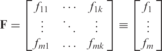
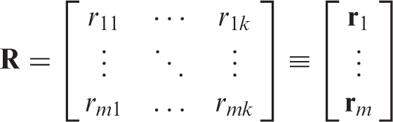
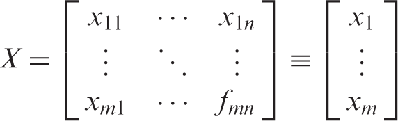
From equation (1), the generated values of f_ij is written in the matrix form as follows

F = \exp (- R^{2} / (2_{m, 1} (σ^{2})^{T}))

(6)

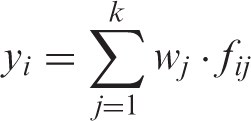
The RBF that is computed by the j ^th hidden unit using equation (1) is maximum, when the input vector x_i is close to the center c_j of that unit. The output of an RBFNN can be computed as a weighted sum of the hidden units⁴⁵

y_{i} = \sum_{j = 1}^{k} w_{j} \cdot f_{ij}

(7)

where w_j is the weight of the j ^th hidden unit for the output and y_i is the output for the i ^th input data.

One of the most important factors affecting the prediction performance of a RBFNN model is the number of neurons because they form the main construction of the RBFNN model. Many methods such as evolutionary algorithms^40,41 and k-fold cross-validation were proposed to determine the number of neurons and their centers.⁴² In our study, a three-fold cross-validation (3CV) method has been used. The method is explained in detail in Section 1.2.4, “Determining the training and testing dataset”.

1.2.2 Implementing the RBFNN method for modeling

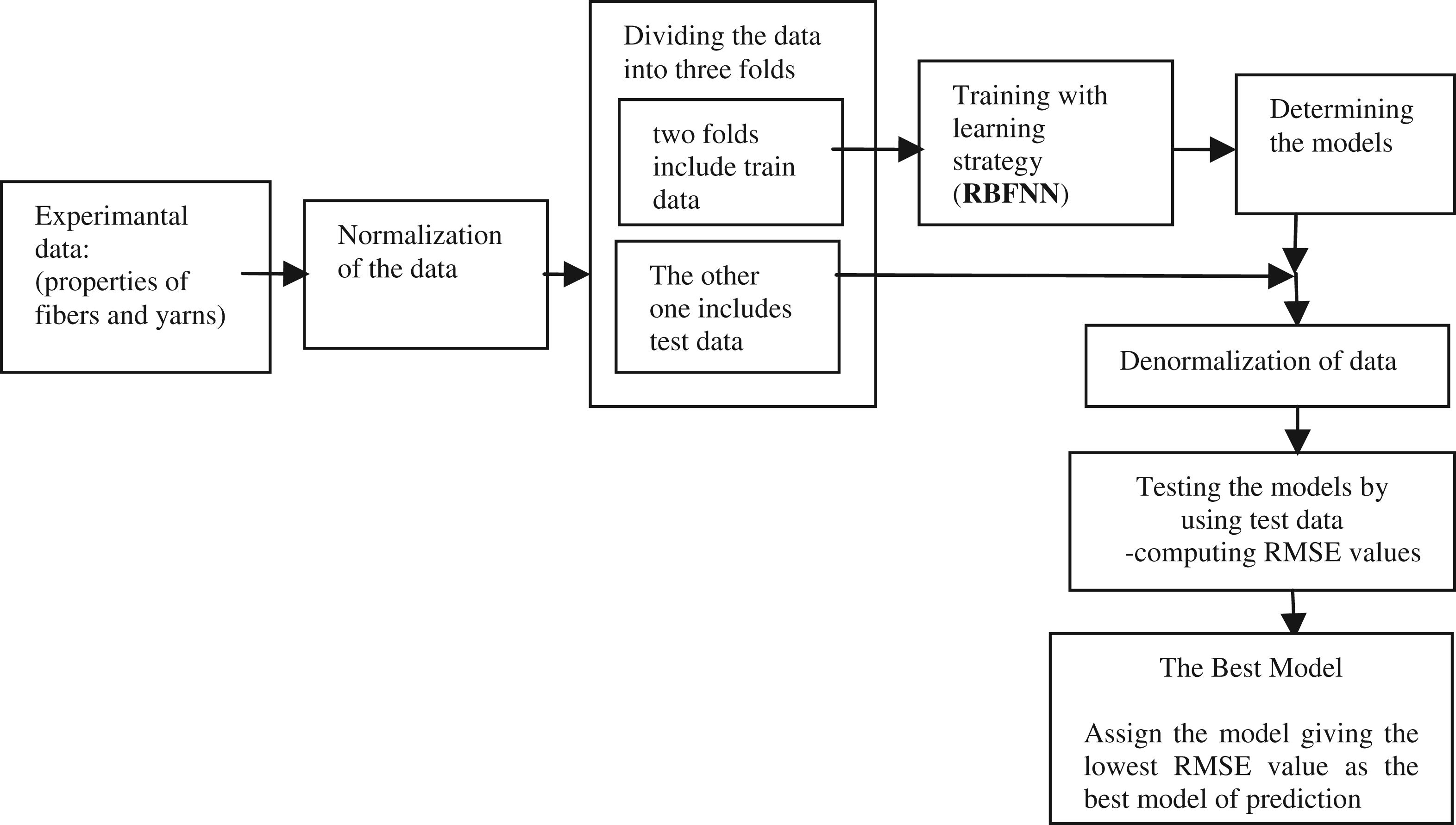
In this method, the yarn tenacity and hairiness values, which were experimentally measured by using USTER tensorapid and Uster tester 3, respectively, were predicted using the RBFNN method. The RBFNN design process involved six steps. These were

1. Determining the input and output dataset from experimental values

2. Determining the training and testing dataset

3. Normalization and renormalization of the data

4. Training

5. Testing the models

6. Determining the best model

7. Creating the stages of modeling, as shown in Figure 2.

Figure 2.

Schematic representation of the modeling study.

1.2.3 Determining the input and output dataset from experimental values

The modeling studies were carried out for four prediction cases. These cases are presented in Table 2.

Table 2.

The four prediction cases for radial basis function neural network modeling

Case	Input data	Output data
Case 1	HVI fiber measurement results + Yarn count	Yarn tenacity
Case 2	AFIS fiber measurement results + Yarn count	Yarn tenacity
Case 3	HVI fiber measurement results + Yarn count	Yarn hairiness
Case 4	AFIS fiber measurement results + Yarn count	Yarn hairiness

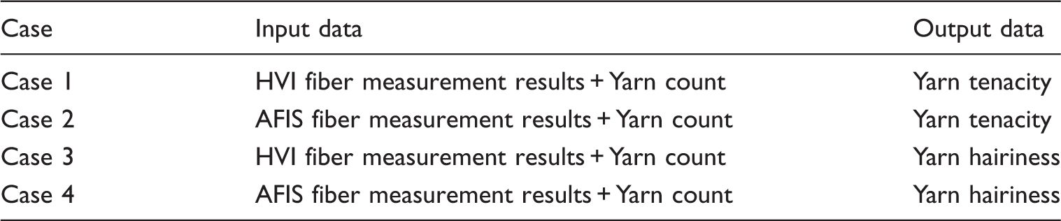
The dataset for the RBFNN modeling was formed by considering the four cases. Table 1 shows the dataset.

1.2.4 Determining the training and testing dataset

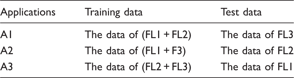
In the modeling study, some of the experimental data was used for training, and the other experimental data was used for testing. Many methods in literature proposed this to select data for training and testing. In this study, a k-fold cross-validation method was applied to select training and testing data for many epochs (epoch refers to each trial and error for decreasing the mean square error (MSE) of the ANN in the batch processing mode) in many numbers of neurons because this method was used successfully in previous applications.^39–41 k-fold cross-validation is a technique to develop the holdout method. In this method, the data set is separated into k subsets, and the holdout method is repeated k times. Each time, one of the k subsets is considered as the test set and the other k - 1 subsets are incorporated to create a training dataset. Then in order to predict accurately, the average error corresponding to k trials is computed. Each data point is included in a test set definitely once and is included in a training set k - 1 times. The variance of the resulting estimate is reduced as k is increased. A variant of this method is to randomly divide the data into a test and training set k times. The advantage of doing this is that we can independently choose how large each test set is and how many trials one averages.^47,48

After many past studies were reviewed, the number of k was determined as three for the number of data in this study. Therefore, a 3CV method was applied to determine the dataset for training and testing. The experimental data was randomly divided into three folds (clusters) containing different values as given in Table 3.

Table 3.

Three randomly chosen folds for the three-fold cross-validation method

Folds (Clusters)
FL1	FL2	FL3
Data line Nr	Data line Nr	Data line Nr
1	2	3
5	4	6
9	7	8
12	11	10
15	14	13
19	18	16
21	22	17
25	24	20
27	26	23
31	28	29
33	30	32
36	34	35
39	38	37
		40

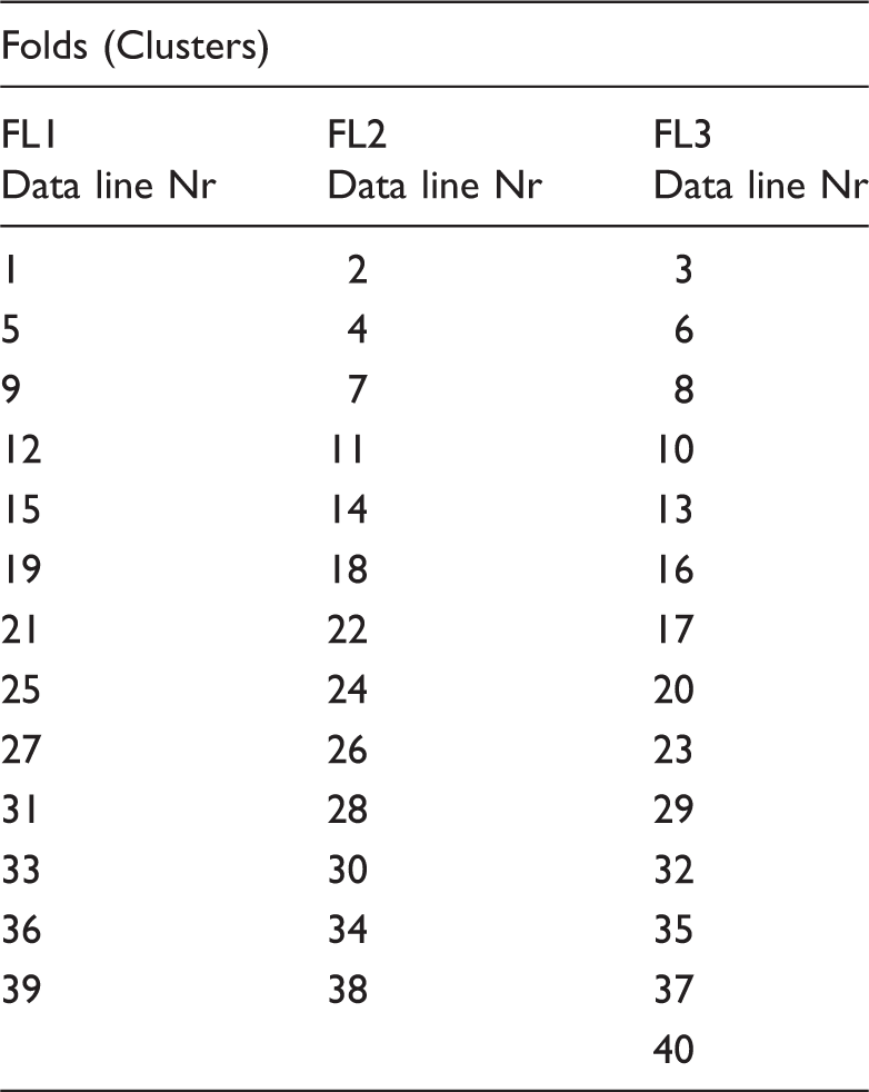
Table 3 was generated from Table 1, and the numbers in Table 3 refer the line numbers of experimental data in Table 1.

In the modeling study, the values belonging to any two of these folds were used as the training data and the values belonging to the other fold were selected as the testing data. Thus, all values were used in both training and testing. In Table 4, the training and test folds are presented. As seen in the table, there are three applications for training and testing clusters. The method was carried out three times. The simulations were performed for between two and 20 different hidden units.

Table 4.

Training and test datasets for the three-fold cross-validation method

Applications	Training data	Test data
A1	The data of (FL1 + FL2)	The data of FL3
A2	The data of (FL1 + F3)	The data of FL2
A3	The data of (FL2 + FL3)	The data of FL1

1.2.5 Normalization and renormalization of the data

The purpose of the normalization of the data is to prevent the higher values to weigh down the influence of lower values and to maintain the symmetry of the activation function. In this study, linear normalization was used. All values in a variable were divided by its maximum value to be normalized to the same range values [0, 1]. After training was performed, normalized network outputs were renormalized back to their original values.

1.2.6 Training

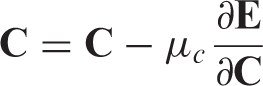
The purpose of an RBFNN model is to carry out a nonlinear function approximation. For this reason, firstly, W, σ, and C are determined by using a supervised learning algorithm. Therefore, the sum squared is minimized by a gradient descent method.⁴⁹ For this purpose, equation (8)⁴⁹ was used

E = \sum_{i = 1}^{m} (y_{i} - {\overset{\land}{y}}_{i})^{2}

(8)

where y_i (measured output data) and

{\overset{\land}{y}}_{i}

(predicted output data) are m × n matrices for the measured training data and RBFNN output, respectively.³⁷

Firstly, all center values were selected randomly, making sure that all of the center values were in the input range. The spread of the j^th center c _j is denoted as σ _j and it is mainly related to the number of RBF functions. The σ vector is given as

σ = [\begin{matrix} σ_{1} \\ : \\ σ_{k} \end{matrix}]

(9)

and initially the elements are all equally taken as⁴³

σ_{j} = \frac{1}{(2 k^{1 / n} - 2) \sqrt{2 \ln 2}} (j = 1, 2, \dots, k)

(10)

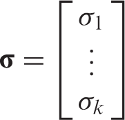
Equation (10) provides an acceptable initial spread in which σ _j increases as the number of input variables increases or the number of hidden units decreases. Initially, all w values were selected randomly. So, the gradient descent learning for the three parameters can be given as⁴³

W = W - μ_{w} \frac{\partial E}{\partial W}

(11)

σ = σ - μ_{σ} \frac{\partial E}{\partial σ}

(12)

C = C - μ_{c} \frac{\partial E}{\partial C}

(13)

where μ_w , µ _r, and µ _c are scalars that represent the learning rate for the related parameter.⁴³

1.2.7 Testing the RBFNN models

Testing of the trained ANN requires the inputs of the test set be presented to the RBFNN. The measured output of the test set is compared to the output produced by the RBFNN in order to see if the RBFNN’s output is acceptable. If the output produced by the trained RBFNN is correct within accepted error ranges, the RBFNN can then be used in modeling the dataset.

The prediction performance is analyzed by using the root mean square error (RMSE) for only single output RBFNN works, which is given as⁴⁹

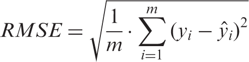
RMSE = \sqrt{\frac{1}{m} \cdot \sum_{i = 1}^{m} (y_{i} - {\overset{\land}{y}}_{i}) 2}

(14)

In this study, the best model that gives the minimum RMSE is determined by comparing RMSE values of the test data.

2. Results and discussion

The results of modeling study are presented in two main stages. These are

Determining the models: This stage contains the following studies:

– Computing RMSE values of each application

– Determining the mean RMSE values of a given epoch

– Determining the minimum mean RMSE value in a given neuron

– Determining the best RBFNN model for a given case

Testing the RBFNN model

After these stages, the RBFNN model was compared with the model developed by using linear regression analysis.

Figure 3 shows the stages of modeling studies for case 1 as an example.

Figure 3.

The stages of modeling studies for case 1.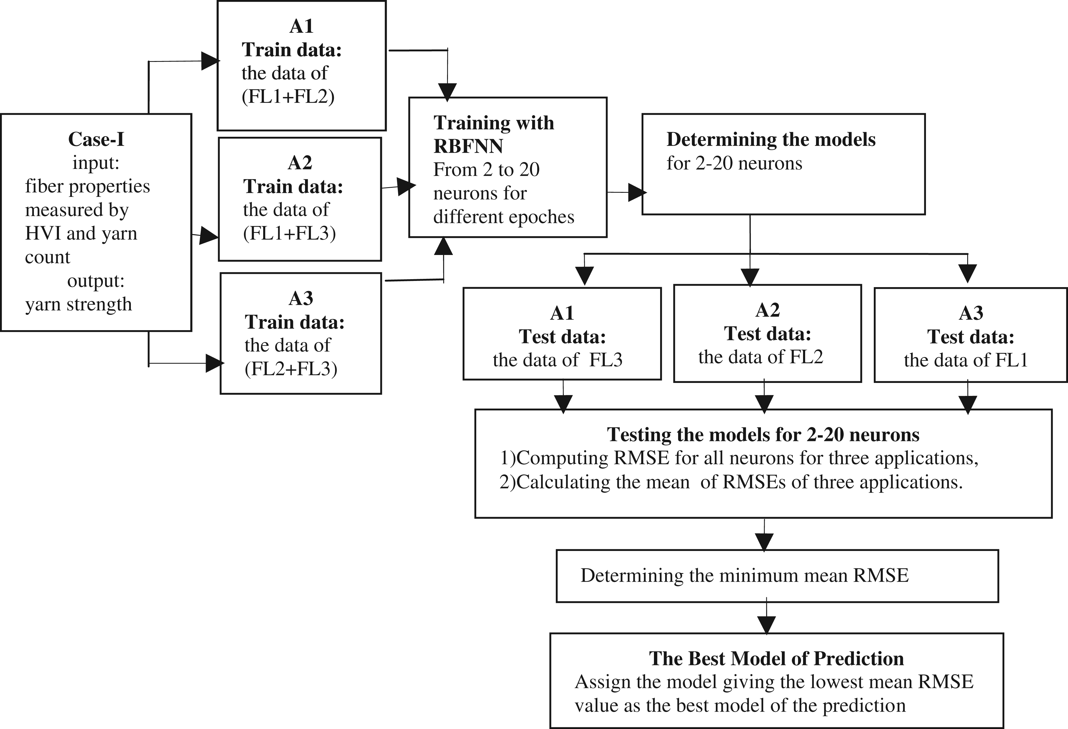

2.1 Determining the models with RBFNN

2.1.1 Computing RMSE values of each application

For determining the prediction models, test and train RMSE values of each three applications were computed in different epochs for a given neuron. As an example, Table 5 presents the parameters selected for the modeling study of case 1. Figure 4 shows the test RMSE and train RMSE values of application 2 (A2) in many epochs of two neurons for case-I.

Figure 4.

The test and training root mean square error (RMSE) values of application-2 (A2) in two neurons for case 1.

Table 5.

The parameters selected for the modeling study of case 1

Case 1
Input data	The fiber properties measured by using HVI and yarn count (Yarn tenacity cN/tex)
Output data
Application	A1	A2	A3
Data for traning	The data of (FL1 + FL2)	The data of (FL1 + FL3)	The data of (FL2 + FL3)
Data for testing	The data of FL3	The data of FL2	The data of FL1
The number of neurons	2,3,4,5,6,7,8,9,10,11,12,	2,3,4,5,6,7,8,9,10,11,12,	2,3,4,5,6,7,8,9,10,11,12,
The number of neurons	13,14,15,16,17,18,19,20	13,14,15,16,17,18,19,20	13,14,15,16,17,18,19,20
Epochs	1000-1,000,000	1000-1,000,000	1000-1,000,000

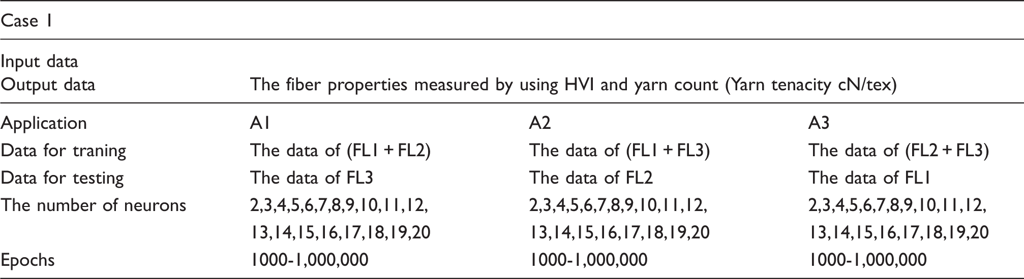
It was observed that the minimum TSTRMSE, the test RMSE, was achieved at epoch 200,000, and the test error started to level-off or increase after that epoch. The test RMSE value at that epoch was then determined to be the RMSE value for this application. The same computations were carried out to find RMSE values of each case corresponding to various neuron configurations. A similar observation was made for all of the other applications of all cases, and therefore, the results were noted up until the epoch value of 200,000.

2.1.2 Determining the mean RMSE values of a given epoch

The mean RMSE values were computed by considering the RMSE values of three applications in a given epoch of a given neuron. In equations (15) and (16), computing the mean RMSE value in 5000 epochs of two neurons for case 1 is presented as an example

Mean of TRNRMS = \frac{{TRNRMSE}_{case 1, 2, 5000, A 1} {+ TRNRMSE}_{case 1, 2, 5000; A 2} {+ TRNRMSE}_{case 1, 2, 5000, A 3}}{3}

(15)

Mean of TSTRMSE = \frac{{TSTRMSE}_{case 1, 2, 5000, A 1} {+ TSTRMSE}_{case 1, 2, 5000; A 2} {+ TSTRMSE}_{case 1, 2, 5000, A 3}}{3}

(16)

where

TRNRMSE is the RMSE value for training data,

TSTRMSE is the RMSE value for test data,

the number of neurons, A1, A2, A3, is the application number, and

Mean of TSTRMSE = $\frac{0, 797 + 0, 769 + 0, 989}{3} = 0, 851$

The mean RMSE values of each epoch in a given neuron were found by the same computing method. In Table 6, the mean TSTRMSE values of each epoch in two neurons for case1 are used as an example.

Table 6.

The mean test root mean square error (TSTRMSE) values of each epoch in two neurons for case 1

The minimum mean RMSE values of test data for case 1
Epoch	5000				10,000				30,000				50,000				80,000				1,00,000				2,00,000
	TSTRMSE for application			mean of	TSTRMSE for application			mean of	TSTRMSE for application			mean of	TSTRMSE for application			mean of	TSTRMSE for application			mean of	TSTRMSE for application			mean of	TSTRMSE for application			mean of
Neurons	A1	A2	A3	RMSE	A1	A2	A3	RMSE	A1	A2	A3	RMSE	A1	A2	A3	RMSE	A1	A2	A3	RMSE	A1	A2	A3	RMSE	A1	A2	A3	RMSE
2	0.80	0.77	0.99	0.85	0.79	0.74	0.98	0.83	0.75	0.69	0.97	0.80	0.62	0.69	0.93	0.75	0.61	0.63	0.86	0.70	0.60	0.63	0.71	0.65	0.48	0.56	0.53	0.52

2.1.3 Determining the minimum mean RMSE value in a given neuron

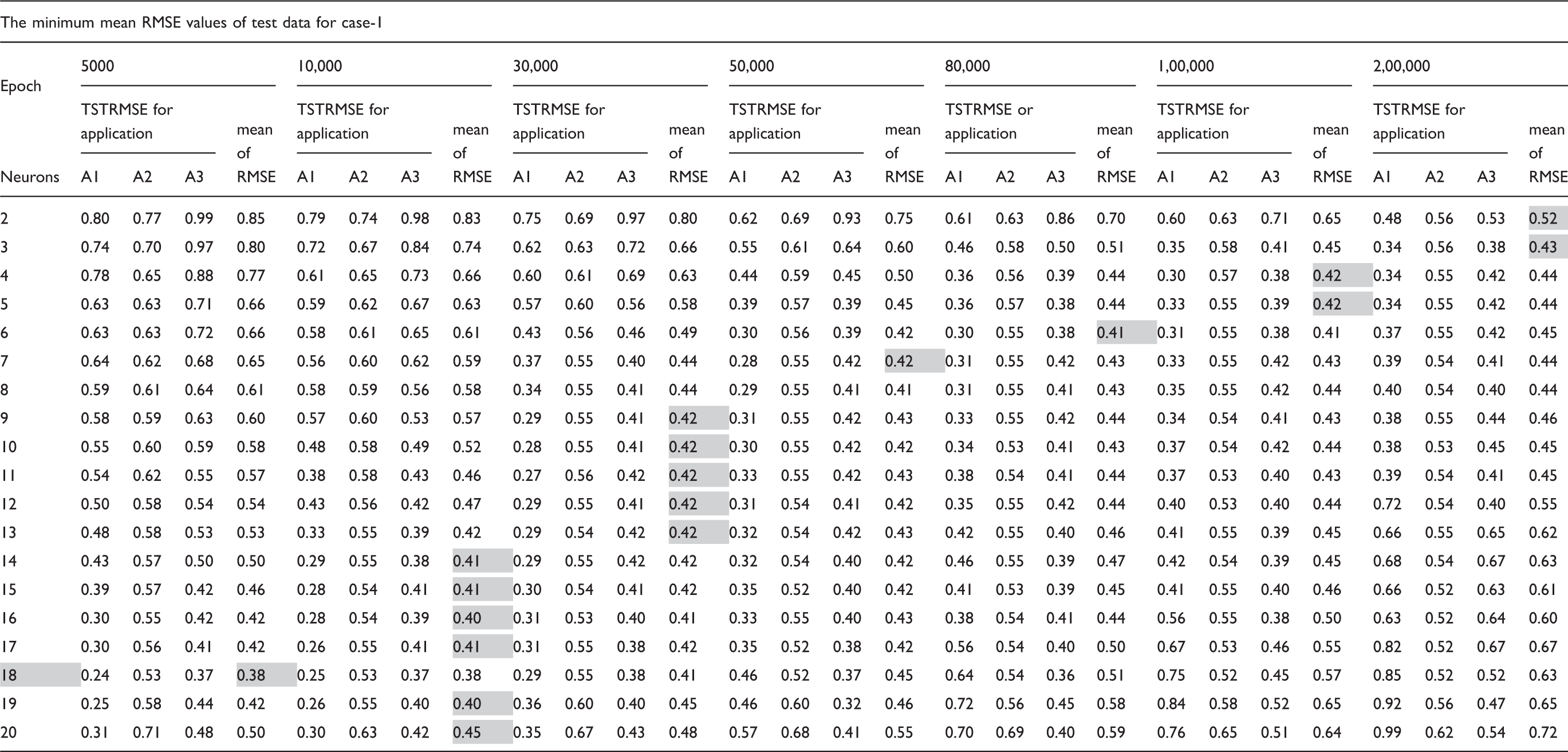
The minimum mean RMSE was determined by comparing all mean RMSE values in a given neuron. The minimum mean TSTRMSE values of each neuron for case1 are introduced in Table 7 as an example.

Table 7.

The minimum mean of test root mean square error (TSTRMSE) values of all of the neurons for case 1

The minimum mean RMSE values of test data for case-1
Epoch	5000				10,000				30,000				50,000				80,000				1,00,000				2,00,000
	TSTRMSE for application			mean of	TSTRMSE for application			mean of	TSTRMSE for application			mean of	TSTRMSE for application			mean of	TSTRMSE or application			mean of	TSTRMSE for application			mean of	TSTRMSE for application			mean of
Neurons	A1	A2	A3	RMSE	A1	A2	A3	RMSE	A1	A2	A3	RMSE	A1	A2	A3	RMSE	A1	A2	A3	RMSE	A1	A2	A3	RMSE	A1	A2	A3	RMSE
2	0.80	0.77	0.99	0.85	0.79	0.74	0.98	0.83	0.75	0.69	0.97	0.80	0.62	0.69	0.93	0.75	0.61	0.63	0.86	0.70	0.60	0.63	0.71	0.65	0.48	0.56	0.53	0.52
3	0.74	0.70	0.97	0.80	0.72	0.67	0.84	0.74	0.62	0.63	0.72	0.66	0.55	0.61	0.64	0.60	0.46	0.58	0.50	0.51	0.35	0.58	0.41	0.45	0.34	0.56	0.38	0.43
4	0.78	0.65	0.88	0.77	0.61	0.65	0.73	0.66	0.60	0.61	0.69	0.63	0.44	0.59	0.45	0.50	0.36	0.56	0.39	0.44	0.30	0.57	0.38	0.42	0.34	0.55	0.42	0.44
5	0.63	0.63	0.71	0.66	0.59	0.62	0.67	0.63	0.57	0.60	0.56	0.58	0.39	0.57	0.39	0.45	0.36	0.57	0.38	0.44	0.33	0.55	0.39	0.42	0.34	0.55	0.42	0.44
6	0.63	0.63	0.72	0.66	0.58	0.61	0.65	0.61	0.43	0.56	0.46	0.49	0.30	0.56	0.39	0.42	0.30	0.55	0.38	0.41	0.31	0.55	0.38	0.41	0.37	0.55	0.42	0.45
7	0.64	0.62	0.68	0.65	0.56	0.60	0.62	0.59	0.37	0.55	0.40	0.44	0.28	0.55	0.42	0.42	0.31	0.55	0.42	0.43	0.33	0.55	0.42	0.43	0.39	0.54	0.41	0.44
8	0.59	0.61	0.64	0.61	0.58	0.59	0.56	0.58	0.34	0.55	0.41	0.44	0.29	0.55	0.41	0.41	0.31	0.55	0.41	0.43	0.35	0.55	0.42	0.44	0.40	0.54	0.40	0.44
9	0.58	0.59	0.63	0.60	0.57	0.60	0.53	0.57	0.29	0.55	0.41	0.42	0.31	0.55	0.42	0.43	0.33	0.55	0.42	0.44	0.34	0.54	0.41	0.43	0.38	0.55	0.44	0.46
10	0.55	0.60	0.59	0.58	0.48	0.58	0.49	0.52	0.28	0.55	0.41	0.42	0.30	0.55	0.42	0.42	0.34	0.53	0.41	0.43	0.37	0.54	0.42	0.44	0.38	0.53	0.45	0.45
11	0.54	0.62	0.55	0.57	0.38	0.58	0.43	0.46	0.27	0.56	0.42	0.42	0.33	0.55	0.42	0.43	0.38	0.54	0.41	0.44	0.37	0.53	0.40	0.43	0.39	0.54	0.41	0.45
12	0.50	0.58	0.54	0.54	0.43	0.56	0.42	0.47	0.29	0.55	0.41	0.42	0.31	0.54	0.41	0.42	0.35	0.55	0.42	0.44	0.40	0.53	0.40	0.44	0.72	0.54	0.40	0.55
13	0.48	0.58	0.53	0.53	0.33	0.55	0.39	0.42	0.29	0.54	0.42	0.42	0.32	0.54	0.42	0.43	0.42	0.55	0.40	0.46	0.41	0.55	0.39	0.45	0.66	0.55	0.65	0.62
14	0.43	0.57	0.50	0.50	0.29	0.55	0.38	0.41	0.29	0.55	0.42	0.42	0.32	0.54	0.40	0.42	0.46	0.55	0.39	0.47	0.42	0.54	0.39	0.45	0.68	0.54	0.67	0.63
15	0.39	0.57	0.42	0.46	0.28	0.54	0.41	0.41	0.30	0.54	0.41	0.42	0.35	0.52	0.40	0.42	0.41	0.53	0.39	0.45	0.41	0.55	0.40	0.46	0.66	0.52	0.63	0.61
16	0.30	0.55	0.42	0.42	0.28	0.54	0.39	0.40	0.31	0.53	0.40	0.41	0.33	0.55	0.40	0.43	0.38	0.54	0.41	0.44	0.56	0.55	0.38	0.50	0.63	0.52	0.64	0.60
17	0.30	0.56	0.41	0.42	0.26	0.55	0.41	0.41	0.31	0.55	0.38	0.42	0.35	0.52	0.38	0.42	0.56	0.54	0.40	0.50	0.67	0.53	0.46	0.55	0.82	0.52	0.67	0.67
18	0.24	0.53	0.37	0.38	0.25	0.53	0.37	0.38	0.29	0.55	0.38	0.41	0.46	0.52	0.37	0.45	0.64	0.54	0.36	0.51	0.75	0.52	0.45	0.57	0.85	0.52	0.52	0.63
19	0.25	0.58	0.44	0.42	0.26	0.55	0.40	0.40	0.36	0.60	0.40	0.45	0.46	0.60	0.32	0.46	0.72	0.56	0.45	0.58	0.84	0.58	0.52	0.65	0.92	0.56	0.47	0.65
20	0.31	0.71	0.48	0.50	0.30	0.63	0.42	0.45	0.35	0.67	0.43	0.48	0.57	0.68	0.41	0.55	0.70	0.69	0.40	0.59	0.76	0.65	0.51	0.64	0.99	0.62	0.54	0.72

2.1.4 Determining the best RBFNN model for a given case

The best neuron, which represented the best prediction model, was determined by selecting the neuron giving the lowest minimum mean TSTRMSE values among all the neurons.

Table 7 presents RMSE values for case1, which is the prediction of yarn tenacity by using HVI fiber measurement results and yarn counts. A detailed analysis of this table leads to the conclusion that the best RBFNN model for case1 is the one with 18 neurons (hidden layers), given the minimum RMSE value.

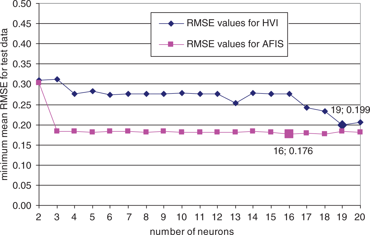
For the other three cases, a detailed RMSE table like Table 6 was built. Upon analysis of the tables, the best networks for these cases have been determined. Figures 4 and 5 summarize these tables for four cases. Figures 5 and 6 show the minimum mean RMSE values and the number of neurons corresponding to them on the prediction of yarn tenacity and on the prediction of yarn hairiness, respectively.

Figure 5.

The minimum mean root mean square error (RMSE) values of test data for predicting yarn tenacity model. HVI: high-volume instrument; AFIS: advanced fiber information system.

Figure 6.

The minimum mean root mean square error (RMSE) values of test data for predicting yarn hairiness model. HVI: high-volume instrument; AFIS: advanced fiber information system.

With a detailed analysis of the figures, for each of the four cases, the lowest minimum mean RMSE value, which represents the best RBFNN mode, can be seen. These values are presented in Table 8.

Table 8.

The best radial basis function neural network model for each of the four cases

Predicted properties	Source of input data	Number of neurons	MM-TSTRMSE
Yarn tenacity (cN/tex)	HVI	18	0.3792
Yarn tenacity (cN/tex)	AFIS	11	0.3757
Yarn hairiness (H)	HVI	19	0.1987
Yarn hairiness (H)	AFIS	16	0.1764

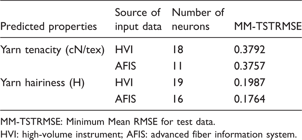
MM-TSTRMSE: Minimum Mean RMSE for test data. HVI: high-volume instrument; AFIS: advanced fiber information system.

It is seen from Figures 4, 5, and 6 and Table 8 that the predicting performance of HVI and AFIS fiber measurements for yarn hairiness is better than the predicting performance for yarn tenacity.

Figure 5 illustrates that the minimum mean TSTRMSE values of predicting yarn tenacity from HVI and AFIS fiber measurement are close but are received in different numbers of neurons.

When Figure 6 is analyzed, it shows that the minimum mean TSTRMSE value of predicting yarn hairiness from AFIS fiber measurements and yarn counts is a bit smaller than that from HVI fiber measurements and yarn counts.

2.2 Testing RBFNN model

The experimental dataset in this section is different from the experimental dataset used for the training and modeling studies. For the testing simulations with the RBFNN using the models in Table 8, the testing dataset was taken, as given in Table 9.

Table 9.

The dataset for testing of the selected radial basis function neural network models

Input data																Output data
		AFIS fiber measurements							HVI fiber measurements							Measured values
Number	Line	Y.C.	L(w)	L(w)	SFC(w)		Mat	Neps	Y.C.		Len2	Uni.	FStr	Elong.	S.F.	Y.S.	Hairiness
of data	Nr.	Ne	mm	%	%	mTex	ratio	Cnt/gr	Ne	microner	mm	%U	gr/tex	%	%	cN/tex	H
1	1	20	25.77	32.40	7.08	165.44	0.88	118.46	20	4.34	30.17	82.22	27.15	6.96	6.95	17.61	7.35
2	5	20	24.70	34.49	8.33	151.38	0.86	234.86	20	3.94	29.64	82.61	30.77	7.03	8.77	19.04	7.36
3	9	20	24.83	33.75	8.99	162.40	0.85	234.23	20	4.14	29.59	83.67	31.86	7.79	7.79	16.75	7.13
4	12	24	25.58	32.89	7.29	162.74	0.87	126.91	24	4.22	30.10	83.03	23.75	7.06	7.51	16.65	6.83
5	15	24	24.70	34.49	8.33	151.38	0.86	234.86	24	3.94	29.64	82.61	30.77	7.03	8.77	18.29	6.87
6	19	24	24.83	33.75	8.99	162.40	0.85	234.23	24	4.14	29.59	83.67	31.86	7.79	7.79	16.50	6.23
7	21	30	25.77	32.40	7.08	165.44	0.88	118.46	30	4.34	30.17	82.22	27.15	6.96	6.95	16.54	6.26
8	25	30	24.70	34.49	8.33	151.38	0.86	234.86	30	3.94	29.64	82.61	30.77	7.03	8.77	18.57	6.29
9	27	30	24.51	33.26	8.84	165.57	0.87	209.34	30	4.18	28.67	82.97	30.11	7.28	8.73	16.59	5.96
10	31	40	25.77	32.40	7.08	165.44	0.88	118.46	40	4.34	30.17	82.22	27.15	6.96	6.95	15.56	5.67
11	33	40	24.68	33.32	8.96	162.17	0.85	267.25	40	4.44	28.86	83.50	27.84	7.09	9.07	15.50	5.92
12	36	40	24.87	34.63	8.44	152.36	0.86	224.15	40	4.18	29.73	82.62	30.70	7.01	8.37	16.96	5.98
13	39	40	24.83	33.75	8.99	162.40	0.85	234.23	40	4.14	29.59	83.67	31.86	7.79	7.79	15.17	5.16
		S.F.: Short fiber index				Y.C.: Yarn count			FStr: Fiber strength				Y.S.: Yarn tenacity

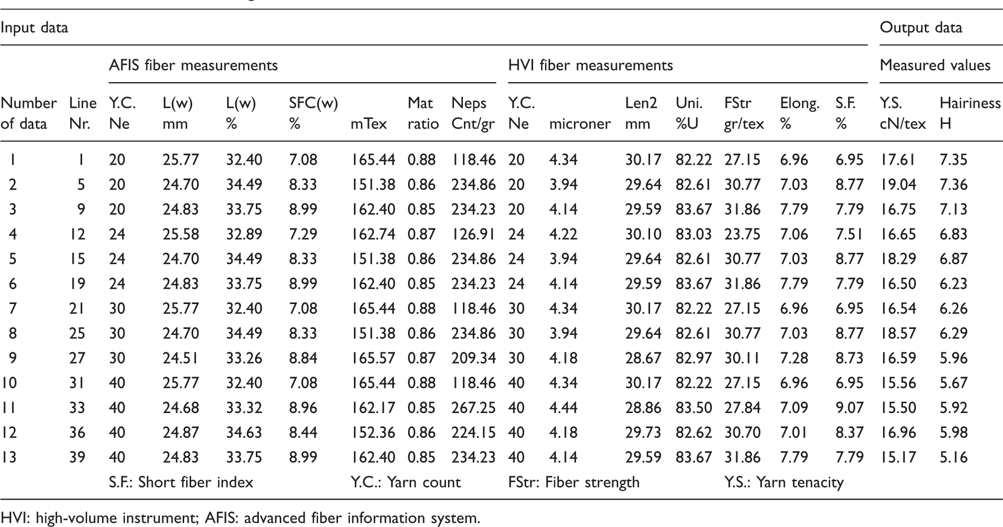
HVI: high-volume instrument; AFIS: advanced fiber information system.

The RMSE values of unseen test data in the best RBFNN models of four cases are shown in Table 10.

Table 10.

The root mean square error (RMSE) values of unseen test data in the best radial basis function neural network models for the four cases

Predicted properties	Source of input data	Number of neurons	RMSE values between experimental- predicted
Yarn tenacity (cN/tex)	HVI	18	0.346
Yarn tenacity (cN/tex)	AFIS	11	0.352
Yarn hairiness (H)	HVI	19	0.158
Yarn hairiness (H)	AFIS	16	0.155

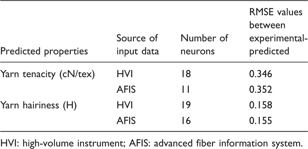
HVI: high-volume instrument; AFIS: advanced fiber information system.

Figures 7 and 8 show the predicted and measured yarn tenacity and yarn hairiness, respectively.

Figure 7.

The predicted and measured yarn tenacity values. HVI: high-volume instrument; AFIS: advanced fiber information system.

Figure 8.

The predicted and measured yarn hairiness values. HVI: high-volume instrument; AFIS: advanced fiber information system.

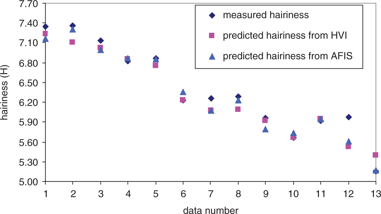
With a detailed analysis of the figures, it can be seen that the measured and predicted values are very close (well correlated) and the changes in curves of measured and predicted values are very similar in both of figures. So, it can be stated that there is no remarkable difference between HVI and AFIS fiber measurements in respect to the predicting performance for these four cases.

2.3 Determining the models by linear regression analyses

Linear regression develops the models that represent the relationship between a scalar variable y and one or more elucidatory variables shown, x. The case of one explanatory variable is called a simple linear regression. More than one explanatory variable is called a multiple linear regression. For this study, multiple regression models were selected because there was more than one independent variable.^44,49 In linear multiple regression, a simple model relates several independent variables to a dependent variable with a straight line given as^44,49

y = β_{0} + β_{1} x_{1} + β_{2} x_{2} + \dots \dots + β_{n} x_{n} + ɛ

(17)

where

y is the predicted output (dependent variable),

x_n is the input data (independent variable),

n is the number of independent variables,

β₀ is the y-intercept of the line,

β_n are the coefficients of the independent variables, and

ε is the random error component.

In this study, linear regression analyses were carried out using SPSS 16.0 program.

2.4 Determining the linear regression model by using the dataset of training

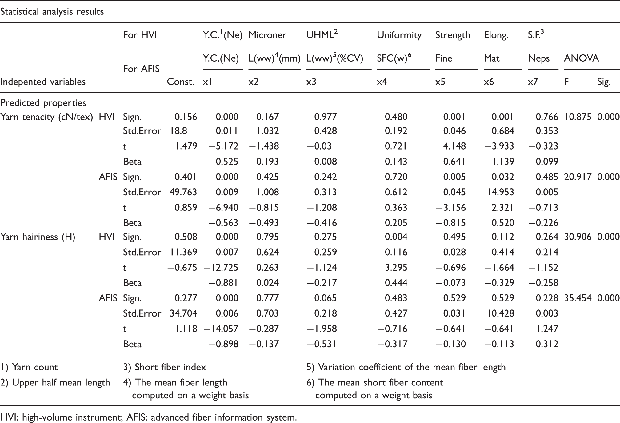
The experimental dataset used in determining the RBFNN models were chosen to train the linear models. In Table 11, the statistical analysis results (regression coefficients of variables, the t-values, significance level of each variable, and beta values) of all cases are introduced. Table 12 shows the linear regression models for all cases.

Table 11.

Statistical analysis results in linear regression analysis

Statistical analysis results
Indepented variables		For HVI	Const.	Y.C.¹(Ne)	Microner	UHML²	Uniformity	Strength	Elong.	S.F.³
		For AFIS		Y.C.(Ne)	L(ww)⁴(mm)	L(ww)⁵(%CV)	SFC(w)⁶	Fine	Mat	Neps	ANOVA
				x1	x2	x3	x4	x5	x6	x7	F	Sig.
Predicted properties
Yarn tenacity (cN/tex)	HVI	Sign.	0.156	0.000	0.167	0.977	0.480	0.001	0.001	0.766	10.875	0.000
		Std.Error	18.8	0.011	1.032	0.428	0.192	0.046	0.684	0.353
		t	1.479	−5.172	−1.438	−0.03	0.721	4.148	−3.933	−0.323
		Beta		−0.525	−0.193	−0.008	0.143	0.641	−1.139	−0.099
	AFIS	Sign.	0.401	0.000	0.425	0.242	0.720	0.005	0.032	0.485	20.917	0.000
		Std.Error	49.763	0.009	1.008	0.313	0.612	0.045	14.953	0.005
		t	0.859	−6.940	−0.815	−1.208	0.363	−3.156	2.321	−0.713
		Beta		−0.563	−0.493	−0.416	0.205	−0.815	0.520	−0.226
Yarn hairiness (H)	HVI	Sign.	0.508	0.000	0.795	0.275	0.004	0.495	0.112	0.264	30.906	0.000
		Std.Error	11.369	0.007	0.624	0.259	0.116	0.028	0.414	0.214
		t	−0.675	−12.725	0.263	−1.124	3.295	−0.696	−1.664	−1.152
		Beta		−0.881	0.024	−0.217	0.444	−0.073	−0.329	−0.258
	AFIS	Sign.	0.277	0.000	0.777	0.065	0.483	0.529	0.529	0.228	35.454	0.000
		Std.Error	34.704	0.006	0.703	0.218	0.427	0.031	10.428	0.003
		t	1.118	−14.057	−0.287	−1.958	−0.716	−0.641	−0.641	1.247
		Beta		−0.898	−0.137	−0.531	−0.317	−0.130	−0.113	0.312
1) Yarn count		3) Short fiber index				5) Variation coefficient of the mean fiber length
2) Upper half mean length		4) The mean fiber length computed on a weight basis				6) The mean short fiber content computed on a weight basis

HVI: high-volume instrument; AFIS: advanced fiber information system.

Table 12.

The models obtained in linear regression analysis

y (Predicted properties)		Prediction models	R ²
Yarn tenacity (cN/tex)	HVI	y = 27.8 + (−0.056)x1 + (−1.484)x2 + (−0.013)x3 + 0.139x4 + 0.192x5 + (−2.692)x6 + (−0.107)*x7	0.80
Yarn tenacity (cN/tex)	AFIS	y = 42.762 + (−0.06)x1 + (−0.821)x2 + (−0.378)x3 + (0.222)x4 + (−0.141)x5 + 34.704x6 + (−0.003)*x7	0.89
Yarn hairiness (H)	HVI	y = (−7.673) + (−0.084)x1 + 0.164x2 + (−0.291)x3 + 0.383x4 + (−0.02)x5 + (−0.689)x6 + (−0.246)*x7	0.92
Yarn hairiness (H)	AFIS	y = 38.813 + (−0.085)x1 + (−0.202)x2 + (−0.428)x3 + (−0.305)x4 + (−0.02)x5 + (−6.682)x6 + 0.004*x7	0.93

HVI: high-volume instrument; AFIS: advanced fiber information system.

From the statistical analysis results in Table 11 and the regression equations in Table 12, it can be seen that the relationships between some fiber characteristics and yarn properties are contrary to expectation. For example, we found a negative effect between fiber elongation results in HVI and yarn tenacity and between mean length results in AFIS and yarn tenacity. The other example is that there is an unexpected negative effect between fiber diameter results in AFIS and yarn hairiness. In addition to the relationship between fiber characteristics and yarn properties, unexpected results were obtained in terms of impact of fiber characteristics on yarn tenacity and hairiness. For example, as known, fiber diameter in AFIS has very high effect on yarn hairiness. However, we found a low influence degree on yarn hairiness for this fiber characteristic. It is the well-known fact that there are very high autocorrelations among fiber properties. These autocorrelations can cause some illogical signs on significant variables of regression equations. Therefore, some of the highly correlated fiber properties should be excluded from the group of independent variables by pre-study before regression analysis. However, in RBFNN modeling, all independent variables were used without considering their autocorrelations between them. Same independent variables were selected for linear regression analyses to compare with RBFNN. Because of the reasons introduced above, the linear regression models achieved in this study can not be used to predict.

2.5 Testing the linear regression model

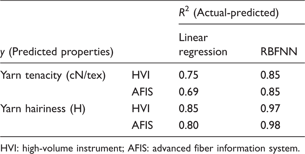
The experimental dataset in the testing of the RBFNN models were used to test the linear models. These values are showed in Table 9. Table 13 presents the correlation coefficients of the RBFNN and linear regression analysis for testing.

Table 13.

Correlation of the coefficients of the radial basis function neural network (RBFNN) and the linear regression analysis for testing

		R ² (Actual-predicted)
y (Predicted properties)		Linear regression	RBFNN
Yarn tenacity (cN/tex)	HVI	0.75	0.85
Yarn tenacity (cN/tex)	AFIS	0.69	0.85
Yarn hairiness (H)	HVI	0.85	0.97
Yarn hairiness (H)	AFIS	0.80	0.98

HVI: high-volume instrument; AFIS: advanced fiber information system.

Figures 9 and 10 show the comparisons between measured output data and output data predicted using the RBFNN and linear regression analysis.

Figure 9.

Comparison between measured and predicted yarn tenacity values for HVI dataset. HVI: high-volume instrument; RBFNN: radial basis function neural network.

Figure 10.

Comparison between measured and predicted yarn tenacity values for AFIS dataset. RBFNN: radial basis function neural network; AFIS: advanced fiber information system.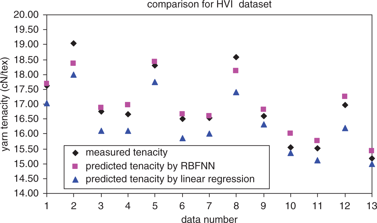

With a detailed analysis of both the HVI and AFIS datasets in these figures and Table 13, it can be noted that the prediction performances of yarn tenacity in RBFNN models are better than those in linear regression models. The information in Table 13 illustrates that the prediction performances of hairiness for both HVIs and AFISs are better than those of the yarn tenacity, similar to RBFNN analysis.

3. Conclusion

An ANN model was developed to predict the strength and hairiness properties of carded cotton yarn. Data generated by using HVI and AFIS fiber measurements were used in an ANN model as input parameters.

The model in this study, both AFIS and HVI input data, performed well at predicting the strength and hairiness properties of carded cotton yarn. For both fiber measurement systems, no significant differences between predicting yarn strength and yarn hairiness were observed.

The results from the ANN model showed that predicting the yarn hairiness is much more accurate compared to predicting the yarn strength. There are two explanations for this. First, as is commonly known, there is a high correlation between yarn hairiness and yarn count. Therefore, yarn count is an important parameter that affects yarn hairiness. The second, and much more important explanation, is the fact that there is an important relation between the coefficient of yarn twist, hairiness, and strength. Additionally, the relationship between the coefficient of twist and yarn strength is stronger than the relationship between the coefficient of twist and yarn hairiness. However, in this study, only one twist factor (4.34α_e) for all yarns was considered. Therefore, tenacity values for all yarns were similar as seen Table 3.

Models can be used for in-house carded cotton yarn development to decrease yarn production cost and time. Also, the RBFNN model has been explained to help researchers who work in this field. This modeling study can be expanded to wider yarn count ranges, other yarn characteristics (e.g., uniformity or neps), different twist factors, and machine settings. Also, taking into account the same characteristics, similar modeling can be carried out for other cotton yarn types, such as combed yarns and open-end yarns.

Footnotes

Acknowledgments

We would like to thank everyone at Abalioglu Yem, Soya and Tekstil Spinning Mill, Denizli, Turkey for their support of our research on fiber measurements of HVIs and AFISs and yarn measurements on Uster systems. We would like to thank Sezai Tokat of Pamukkale University, Computer Engineering Department, in Turkey for his help with the ANN modeling system.

Funding

This research received no specific grant from any funding agency in the public, commercial, or not-for-profit sectors.

References

Vasconcelos

. A knowledge-based system for spinning management. Tex Res J 1996; 66(4): 265–268.

Ethridge

Towery

Hembree

. Estimating functional relationships between fiber properties and strength of open-end spun yarns. Tex Res J 1982; 52(1): 35–45.

El Mogahzy

Broughton

Lynch

. A statistical approach for determining the technological value of cotton using hvi fiber properties. Tex Res J 1990; 60(9): 495–500.

Ewald

Landstreet

. A new method for predicting cotton yarn strength from the observed strength of a single count. Tex Res J 1954; 24: 1064–1068.

Verbeck

. A statistical method of characterizing spinning quality. Tex Res J 1965; 35(1): 1–13.

Ureyen

Kadoglu

. Regressional estimation of ring cotton yarn properties from HVI fiber properties. Tex Res J 2006; 76(5): 360–366.

Ureyen ME and Kadoglu H. The prediction of cotton ring yarn properties from AFIS fibre properties by using linear regression models. Fibres Text East Eure 2007; 63–67.

Dayik

. Prediction of yarn properties using evaluation programing. Tex Res J 2009; 79(11): 963–972.

Majumdar

. Predicting the breaking elongation of ring-spun cotton yarns using mathematical, statistical, and artificial neural network models. Tex Res J 2004; 74(7): 652–655.

10.

Aggarwal

. A model to estimate the breaking elongation of high twist ring-spun cotton yarns: part I: derivation of the model for yarns from single cotton varieties. Tex Res J 1989; 59(11): 691–695.

11.

Aggarwal

. A model to estimate the breaking elongation of high twist ring-spun cotton yarns: part II: applicability to yarns from mixtures of cottons. Tex Res J 1989; 59(12): 717–720.

12.

Zurek

Frydrych

Zakrzewski

. A method of predicting the strength and breaking strain of cotton yarn. Tex Res J 1987; 57(8): 439–444.

13.

Bogdan

. The prediction of cotton yarn strengths 1. Tex Res J 1967; 37: 536–537.

14.

Hafez

OMA

. Yarn-strength prediction of American cottons. Tex Res J 1978; 48: 701–705.

15.

Frydrych

. Strength of cotton blend yarns. Tex Res J 1994; 64: 198–208.

16.

Frydrych

Matusiak

. Predicting the nep number in cotton yarn-determining the critical nep size. Tex Res J 2002; 72(10): 917–923.

17.

Hagan

Demuth

Beale

. Neural network design, Boston: PWS Publishing Company, 2002.

18.

. Dynamic system identification via recurrent multilayer perceptions. Inf Sci 2002; 147: 45–63.

19.

Guruprasada

Behera

. Soft computing in textiles. Indian J Fibre Text Res 2010; 35(1): 75–84.

20.

Zeng

Wang

. Predicting the tensile properties of air-jet spun yarns. Tex Res J 2004; 74(8): 689–689.

21.

Babay

Cheikhrouhou

Vermeulen

. Selecting the optimal neural network architecture for predicting cotton yarn hairiness. J Tex Ins 2004; 96: 185–185.

22.

Furferi R and Gelli M. Yarn strength prediction: a practical model based on artificial neural networks. Adv Mech Eng Epub ahead of print 2010; Volume 2010, Article ID 640103, 11 pages, doi:10.1155/2010/640103; (Accessed: 15 Nov 2011).

23.

Gharehaghaji

Shanbeh

Palhang

. Analysis of two modeling methodologies for predicting the tensile properties of cotton-covered nylon core yarns. Tex Res J 2007; 77(8): 565–565.

24.

Yadav

Kothari

. Prediction of air-jet textured yarn properties using a statistical method and neural network. Indian J Fibre Text Res 2004; 29: 157–162.

25.

Beltran

Wang

. Predicting worsted spinning performance with an artificial neural network model. Tex Res J 2004; 74(9): 757–757.

26.

Ramesh

Rajamanickam

Jayaraman

. The prediction of yarn tensile properties by using artificial neural networks. J Tex Ins 1995; 86(3): 459–469.

27.

Shanbeh M, Hasani H and Tabatabaei SA. Modelling and predicting the breaking strength and mass irregularity of cotton rotor-spun yarns containing cotton fiber recovered from ginning process by using artificial neural network algorithm. Model Simul Eng Epub ahead of print 2011 Volume 2011: Article ID 591905, 8 pages; doi:10.1155/2011/591905; (Accessed 12 Jan 2012).

28.

Desai

Kane

Bandyopadhayay

. Neural networks: an alternative solution for statistically based parameter prediction. Tex Res J 2004; 74(3): 223–223.

29.

Ureyen

Gürkan

. Comparison of artificial neural network and linear regression models for prediction of ring-spun yarn properties: I. prediction of yarn tensile properties. Fibers Polym 2008; 9(1): 87–91.

30.

Ureyen

Gürkan

. Comparison of artificial neural network and linear regression models for prediction of ring-spun yarn properties. ıı. prediction of yarn hairiness and unevenness. Fibers Polym 2008; 9(1): 92–96.

31.

Khan

. An Artificial Neural Network-based Hairiness Prediction Model for Worsted Wool Yarns. Tex Res J 2009; 79(8): 714–720.

32.

Cheng

Adams

. Yarn strength prediction using neural networks part i: fiber properties and yarn strength relationship. Tex Res J 1995; 65(9): 495–500.

33.

Mwasiagi

Huang

Wang

. Performance of neural network algorithms during the prediction of yarn breaking elongation. Fibers Polym 2008; 9(1): 80–86.

34.

Zong-yi X, Yong Q, Xue-miao P, et al. Modelling of the automatic depth control electrohydraulic system using RBF neural network and genetic algorithm. Math Prob Eng Epub ahead of print 2010; Volume 2010; Article ID 124014; 16 pages, doi:10.1155/2010/124014; (Accessed: 20 Nov 2011).

35.

Kim

Park

Choi

. Control of chaotic dynamical systems using radial basis function network approximators. Inf Sci 2000; 130: 165–183.

36.

Meghabghab

Kandel

. Stochastic simulations of web search engines: RBF versus second-order regression models. Inf Sci 2004; 159: 1–28.

37.

Rein

Reisslein

. Identifying the classical music composition of an unknown performance with wavelet dispersion vector and neural nets. Inf Sci 2006; 176(12): 1629–1655.

38.

Toprakci O. A research on the prediction of yarn properties from cotton fiber properties on ring spinning. MSc Thesis, Pamukkale University, Turkey 2008.

39.

Turhan

Eren

Tokat

. Statistical and computational intelligence tools for the analyses of warp tension in different back-rest oscillations. Inf Sci 2007; 177: 5237–5252.

40.

Rivas

Merelo

Castillo

. Evolving RBF neural networks for time-series forecasting with EvRBF. Inf Sci 2004; 165(3–4): 207–220.

41.

Sheta

Jong

. Time-series forecasting using GA-tuned radial basis functions. Inf Sci 2001; 133(3–4): 221–228.

42.

Orr MJL. Regularisation in the selection of radial basis function centres. Neural Computation 1995; 7(3): 606–623.

43.

Jang

Sun

Mizutani

. Neuro-fuzzy and soft computing, Upper Saddle River, NJ: Prentice Hall, 1997.

44.

Chapra

Canale

. Numerical methods for engineers, New York: McGraw-Hill, 2005.

45.

Haykin

. Neural networks: A comprehensive foundation, 2nd edn. Upper Saddle River, NJ: Prentice Hall, 1999, pp. 256–312.

46.

Eberhard Karls Tübingen University. Mathematisch and Naturwissenschaftliche Fakultet, http://www.ra.cs.uni-tuebingen.de/SNNS/UserManual/node175.html (Accessed: 10 Jan 2012).

47.

Polat

Gunes

. An expert system approach based on principal component analysis and adaptive neuro-fuzzy inference system to diagnosis of diabetes disease. Dig Sign Proc 2007; 17: 702–710.

48.

Schneider J. Home page, http://www.cs.cmu.edu/~schneide/tut5/node42.html (2006, accessed September 2006) (Accessed: 16 Jan 2012).

49.

Mendenhall

Sincich

. Statistics for engineering and the science, 4th edn. Upper Saddle River, NJ: Prentice Hall, 1995, pp. 531–615.