Diffusion coefficient calculated by time-lag using the film-roll method

Abstract

A method for determining the diffusion coefficient by time-lag using the film-roll method for the sublimation diffusion of disperse dye was proposed. A polyethylene terephthalate film-roll coated with dye paste was treated at 170–190°C for various times. A solution consisting of the sum of a steady-state solution and a transient solution was obtained by the homogeneous boundary value problem from a trigonometrical series. The boundary conditions of the steady-state first layer and the steady-state first layer amount of dye were determined from the steady-state concentration distribution. For various diffusion times, the steady-state first layer-passed total amounts of dye that passed through the first layer in the steady-state condition were obtained by subtracting the steady-state first layer amounts from the total amounts. The time-lag was calculated from the linear regression line for the plot of the steady-state first layer-passed total number(X) of positive values against time. The diffusion coefficient was calculated by the boundary conditions of the steady-state first layer and the time-lag. For diffusion at 170°C, 180°C, and 190°C, the correlations of the steady-state first layer-passed total amounts with respect to time were very linear and the reliability of the diffusion coefficients obtained by the time-lag was proved by the good linearity of the Arrhenius plot. The activation energy obtained was 36.8 kcal $·$ mol⁻¹.

Keywords

Diffusion printing dyeing sorption color finishing

Diffusion coefficients can be determined both in a non-steady-state and in a steady-state from the solutions obtained by the separation of the variables or by the Laplace transform.¹ The diffusion coefficients determined in a non-steady-state are much more difficult to interpret without ambiguity than measurements in a steady-state.² Dye diffusion in polyethylene terephthalate (PET) film using supercritical carbon dioxide has been studied using the film-roll method by Sicardi et al.³,⁴ The film-roll method measures the concentration–distance profile by which the total amount of dye diffused through the film in a specified time can be easily determined. It has also been used by several researchers in water impregnating systems to evaluate diffusion coefficients of nonionic dyes in synthetic polymers.^5–8

The film-roll method to study the kinetic behavior of vat dyes in cellulose was applied by Sekido and Matsui.⁹ They calculated diffusion coefficients by the ratio of the mean concentrations between adjacent layers and $ζ = ε / \sqrt{4 D t}$ obtained by $ierfc (i ζ)$ in Equation (1), where $\bar{C_{i}}$ is the mean concentration in the $i$ th layer, $ierfc (i ζ)$ is the iterated complementary error function for $i ζ$ , $D$ is the diffusion coefficient, $t$ is time, and $ε$ is the thickness of the layer

\frac{\bar{C_{i + 1}}}{\bar{C_{i}}} = \frac{ierfc (i ζ) - ierfc [(i + 1) ζ]}{ierfc [(i - 1) ζ] - ierfc (i ζ)}

(1)

For the fixation of disperse dyes on PET at atmospheric pressure, the curing of digital textile printing is done at a temperature range of 160–170°C, the high temperature steaming of common printing is done at 170–180°C, and the heat fixation of Thermosol dyeing is done at 180–200°C. In a previous study on the factors affecting the diffusion of disperse dye in print paste on PET film using the film-roll method, it was found that dye passed through more than two layers by steaming at above 170°C and passed through eight layers by steaming at 190°C for 3 hours.¹⁰ Thus, in a subsequent study on the diffusion coefficient for the sublimation diffusion of disperse dye to PET film using the film-roll method, the heat fixation was performed at 170–190°C and the diffusion coefficients were calculated by Equation (1) in the non-steady state.¹¹ A linear function of $- \log D$ with respect to the reciprocal of absolute temperature ( $T^{- 1})$ , that is, an Arrhenius plot, is represented by Equation (2), where $E_{a}$ is the activation energy and $R$ is the gas constant. However, the correlation coefficient of the linear regression line for the Arrhenius plot of the diffusion coefficients obtained by Equation (1) was about 0.96, which indicates a poor linear relationship. The reliability of the diffusion coefficients obtained by Equation (1) was not justifiable. Thus, a reliable method to evaluate the diffusion coefficients using the film-roll method was required

d (- \log D) = \frac{0.434 E_{a}}{R} d (T^{- 1})

(2)

In a recent study on diffusion using the film-roll method, the diffusion coefficient was calculated by obtaining the variable $x / \sqrt{4 D t}$ of the complementary error function $erfc (x / \sqrt{4 D t})$ from the ratio of the concentration $C_{x}$ at distance $x$ to the surface concentration $C_{1}$ , that is, $C_{x} / C_{1}$ , at a specified time.¹² The Arrhenius plots for the diffusion of 3 hours and the diffusion of 4 hours showed good linearity, but the standard deviation of the inter-layer diffusion coefficients for the diffusion of 190°C and 3 hours was large.

In another recent study, the solution technique for the diffusion equation using the Fourier series was used to study the calculation of the diffusion coefficient for the sublimation diffusion of disperse dye using the film-roll method.¹³ When an approximate steady-state condition was set up, the diffusion coefficients were calculated by the surface concentration, the total amount of dye, and the steady-state diffusion length for the diffusion at time to reach an approximate steady-state condition. The correlation coefficient of the Arrhenius plot for the diffusion coefficients obtained from the steady-state concentration distribution was almost 1. The reliability of the diffusion coefficients calculated by the equation deduced from the Fourier series was proved by the good linearity of the Arrhenius plot.

In this study, a method for determining the diffusion coefficient by time-lag using the film-roll method for the sublimation diffusion of disperse dye was proposed. PET film-roll coated with dye paste was treated at 170–190°C for various times. The solution of the diffusion equation was obtained by the homogeneous boundary value problem from a trigonometrical series. The time-lag was calculated from the linear regression equation obtained by plotting the steady-state first layer-passed total amount, which is the total amount of dye passed through the steady-state first layer in a certain time on the premise that the first layer boundary conditions are constants, against time. The diffusion coefficient was calculated by the boundary conditions of the first layer and the time-lag. The reliability of the diffusion coefficients obtained by the time-lag was proved by the linearity of the Arrhenius plot. While the diffusion coefficients in two previous studies were obtained for diffusion at a specified time, the diffusion coefficient by time-lag in this study was obtained for the diffusion at several times, including the time to reach an approximate steady-state condition.

Materials and method

Materials

Biaxially oriented PET film (40 μm in thickness) was supplied by SKC. C. I. Disperse Violet 26 (Sumicaron Bordeaux SE-BL) was used without purification. Sodium alginate of the first grade was used.

Preparation of the film-roll

PET film of 40 μm in thickness, of which the width is 4 cm and the length is 50 cm, was wrapped tightly around a glass rod of 2 cm in diameter. Both sides of the film-roll were wrapped by aluminum tape of which the thickness is 30 μm. The printing paste was composed of 300 g of C. I. Disperse Violet 26 and 700 g of 5% (w/w) sodium alginate stock paste.

Sodium alginate paste containing disperse dye was coated on the film-roll between both barriers of aluminum tape, where the thickness of the coated printing paste is 180 μm, and dried at 100°C for 10 minutes in a dryer. The top of the roll was fixed firmly by thin aluminum tape and a glass rod for dividing layers was tied with cotton yarn at both sides of the roll. Figure 1 shows a schematic image of the film-roll and the process of the film-roll method.

Figure 1.

Schematic image of the film-roll. PET: polyethylene terephthalate.

Sublimation condition

The film-roll coated with printing paste was treated in laboratory curing chamber without supplying steam for the sublimation of disperse dye. The heat treatment of 180°C and 190°C was performed for 30-240 minutes. Also, that of 170°C was performed for 60-300 minutes. When the heat treatment was finished, the film was unrolled, washed with water, and cut into the section pieces representing the successive layers.

Determination of dye concentration

The section piece of each film layer (4 $cm \times 3 cm$ ) was dipped in a test tube including chlorobenzene of 20 mL for the extraction of disperse dye. The extraction of dye was performed with boiling chlorobenzene at 132°C until the dye was completely extracted. The dye concentration $(mg / {cm}^{3})$ was calculated by the calibration curve and the optical density of $λ_{\max}$ using a spectrophotometer (Agilent Cary 8454).¹⁴

Results and discussion

Separation of variables and the Fourier series

The sublimation diffusion of disperse dye is the process by which dye is transported from one part of a system to another as a result of random molecular motions.¹⁵ In one-dimensional homogeneous diffusion, when there is a gradient of concentration only along the direction of $x$ and the diffusion coefficient $D$ is constant, the diffusion equation for dye concentration $C (x, t)$ at time $t$ is given by the following equation

\frac{\partial C (x, t)}{\partial t} = D \frac{\partial^{2} C (x, t)}{\partial x^{2}} for t \in [0, \infty), x \in [0, l]

(3)

The separation of variables can be used to obtain a solution of diffusion equation (3) because Equation (3) contains partial derivatives of time $t$ and distance $x$ variables. Substituting $C (x, t) = X (x) T (t)$ into Equation (3) and rearranging it yields Equation (4), where $X (x)$ is a function of only $x$ and $T (t)$ is a function of only $t$ ¹⁶,¹⁷

\frac{1}{T (t)} \frac{d T (t)}{d t} = \frac{D}{X (x)} \frac{d^{2} X (x)}{d x^{2}} = - λ^{2} D

(4)

The first-order ordinary differential equation (ODE) on $T (t)$ in Equation (4) depends only on $t$ and the second-order ODE on $X (x)$ depends only on $x$ so that both ODEs must be equal to the same constant, that is, $- λ^{2} D$ , where $λ$ is constant. The solution of the first-order ODE is $T (t) = e^{- λ^{2} D t}$ and that of the second-order ODE is $X (x) = A \sin (λ x) + B \cos (λ x)$ from the Euler’s Formula where $A$ and $B$ are constants of integration. Thus, the general solution $C (x, t)$ is given by the following equation

C (x, t) = [A \sin (λ x) + B \cos (λ x)] e^{- λ^{2} D t}

(5)

Since the diffusion equation is linear, any finite linear combination of solutions of Equation (5) are also a solution. Therefore, from the principal of superposition and the Fourier series, the general solution is given by the following equation, where $m$ is a positive integer

C (x, t) = \sum_{m = 1}^{\infty} [A_{m} \sin (λ_{m} x) + B_{m} \cos (λ_{m} x)] e^{- {λ_{m}}^{2} D t}

(6)

In Equation (6), $A_{m}$ , $B_{m}$ , and $λ_{m}$ (6) are determined by the initial and boundary conditions for a particular diffusion in a rod of which the side is insulated. When the initial condition is $C (x, 0) = f (x)$ for $0 < x < l$ and the boundary conditions are $C (0, t) = C_{1}$ and $C (l, t) = C_{2}$ for $0 < t < \infty$ , where $C_{1}$ and $C_{2}$ are constants, and if no diffusant can escape through the side, the idealized physical setting for diffusion in a rod is given by Figure 2.¹⁸

Figure 2.

Initial and boundary conditions for diffusion in a rod.

Homogeneous boundary value problem

In the case of the homogeneous boundary value problem for the diffusion equation, the boundary conditions are $C (0, t) = C (l, t) = 0$ in Figure 2, that is, $C_{1} = C_{2} = 0$ . Then $C (0, t) = 0$ yields $B_{m} = 0$ and $C (l, t) = 0$ yields $λ_{m} = m π / l$ . Therefore, by the initial condition $C (x, 0) = f (x)$ for $0 < x < l$ , $f (x)$ in Equation (6) is given by the following equation¹⁸

f (x) = \sum_{m = 1}^{\infty} A_{m} \sin (\frac{m π x}{l})

(7)

Let both sides of Equation (7) be multiplied by $\sin (p π x / l)$ , where $p$ is a positive integer, and be integrated from $0$ to $l$ . Then the integration of the right-hand side becomes zero for $p \neq m$ , but it becomes $A_{m} l / 2$ for $p = m$ , as shown in the following equation

\int_{0}^{l} f (x) \sin (\frac{p π x}{l}) d x = \sum_{m = 1}^{\infty} A_{m} \int_{0}^{l} \sin^{2} (\frac{m π x}{l}) d x = \sum_{m = 1}^{\infty} A_{m} \frac{1}{2} {[x - \frac{l}{2 m π} \sin (\frac{2 m π x}{l})]}_{0}^{l} = A_{m} \frac{l}{2}

(8)

Therefore, substituting $B_{m} = 0$ , $λ_{m} = m π / l$ , and the Fourier sine series coefficients $A_{m}$ of Equation (8) into Equation (6) yields the following equation¹⁹

C (x, t) = \sum_{m = 1}^{\infty} A_{m} \sin (\frac{m π x}{l}) e^{- \frac{m^{2} π^{2} D t}{l^{2}}} = \frac{2}{l} \sum_{m = 1}^{\infty} \sin (\frac{m π x}{l}) e^{- \frac{m^{2} π^{2} D t}{l^{2}}} \int_{0}^{l} f (x) \sin (\frac{m π x}{l}) d x

(9)

If the initial condition is $f (x) = C_{0}$ for $\forall x \in [0, l]$ , $A_{m}$ becomes as follows

A_{m} = \frac{2}{l} \int_{0}^{l} C_{0} \sin (\frac{m π x}{l}) d x = \frac{2 C_{0}}{π} [\frac{1 - \cos (m π)}{m}]

When $f (x) = C_{0}$ , $A_{m}$ is zero for $m = 2, 4, \dots = 2 n$ and $4 C_{0} / [π (2 n + 1)]$ for $m = 1, 3, \cdot \cdot \cdot = 2 n + 1$ from Equation (10) where $n$ is an integer. Thus, Equation (9) becomes the following equation¹⁷

C (x, t) = \frac{4 C_{0}}{π} \sum_{n = 0}^{\infty} \frac{1}{2 n + 1} \sin [\frac{(2 n + 1) π x}{l}] e^{- \frac{{(2 n + 1)}^{2} π^{2} D t}{l^{2}}}

(11)

Steady-state solution and transient solution

In the case of diffusion through a plane sheet, such as a film of thickness $l$ , if the boundary conditions are $C (0, t) = C_{1}$ and $C (l, t) = C_{2}$ for $0 < t < \infty$ and if the initial condition is $C (x, 0) = f (x)$ for $0 < x < l$ , then the corresponding boundary value problem is as follows

{\begin{cases} \frac{\partial C (x, t)}{\partial t} = D \frac{\partial^{2} C (x, t)}{\partial x^{2}} & for t \in [0, \infty), x \in [0, l] \\ C (0, t) = C_{1}, C (l, t) = C_{2} & for 0 < t < \infty \\ C (x, 0) = f (x) & for 0 < x < l \end{cases}

(12)

After a long time, when a steady-state condition is achieved, the gradient of concentration is constant at all points of the plane sheet. There will be no accumulation in the steady-state film layer and the concentration at any point in the steady-state film layer does not change with time even if there was a flow of dye into and out of the film. Let a steady-state concentration distribution, that is, a steady-state solution, be $v (x)$ . Here, $v (x)$ is independent of time and the initial condition. Before a steady-state condition is set up, the solution of Equation (12) changes according to the transient solution $w (x, t)$ , which tends to zero under a steady-state condition. Thus, $C (x, t)$ for Equation (12) is given by the following equation²⁰

C (x, t) = v (x) + w (x, t)

(13)

Substituting

C (x, t) = v (x) + w (x, t)

into Equation (12) yields the following equation

{\begin{cases} \frac{\partial w (x, t)}{\partial t} = D \frac{\partial^{2} [v (x) + w (x, t)]}{\partial x^{2}} & f o r t \in [0, \infty), x \in [0, l] \\ v (0) + w (0, t) = C_{1}, v (l) + w (l, t) = C_{2} & f o r 0 < t < \infty \\ v (x) + w (x, 0) = f (x) & f o r 0 < x < l \end{cases}

(14)

Figure 3 shows the initial and boundary conditions for the solution $C (x, t) = v (x) + w (x, t)$ of Equations (12) and (14) in a plane sheet. A steady-state solution $v (x)$ is a linear function satisfying $v (0) = C_{1}$ and $v (l) = C_{2}$ , as shown in Figure 3. Hence, $v (x)$ is given by the following equation

v (x) = \frac{C_{2} - C_{1}}{l} x + C_{1}

(15)

Figure 3.

Initial and boundary conditions for diffusion in a sheet.

Since $\partial^{2} v (x) / \partial x^{2} = 0$ and $w (0, t) = w (l, t) = 0$ are resulted from Equations (14) and (15), $w (x, t)$ satisfies the homogeneous boundary value problem for the diffusion equation, as shown in the following equation

{\begin{cases} \frac{\partial w (x, t)}{\partial t} = D \frac{\partial^{2} w (x, t)}{\partial x^{2}} for t \in [0, \infty), x \in [0, l] \\ w (0, t) = w (l, t) = 0 for 0 < t < \infty \\ w (x, 0) = f (x) - v (x) for 0 < x < l \end{cases}

(16)

For the homogeneous boundary value problem, that is, $w (0, t) = w (l, t) = 0$ , $C (x, t)$ and $f (x)$ in Equation (9) can be substituted by $w (x, t)$ and $w (x, 0)$ , respectively. Thus, $w (x, t)$ is given by the following equation

w (x, t) = \sum_{m = 1}^{\infty} A_{m} \sin (\frac{m π x}{l}) e^{- \frac{m^{2} π^{2} D t}{l^{2}}} = \frac{2}{l} \sum_{m = 1}^{\infty} \sin (\frac{m π x}{l}) e^{- \frac{m^{2} π^{2} D t}{l^{2}}} \int_{0}^{l} w (x, 0) \sin (\frac{m π x}{l}) d x

(17)

Since $w (x, 0) = f (x) - v (x)$ , $A_{m}$ in Equation (17) becomes as follows

A_{m} = \frac{2}{l} \int_{0}^{l} [f (x) - v (x)] \sin (\frac{m π x}{l}) d x = \frac{2}{l} \int_{0}^{l} f (x) \sin (\frac{m π x}{l}) d x - \frac{2}{l} \int_{0}^{l} v (x) \sin (\frac{m π x}{l}) d x = \frac{2}{l} \int_{0}^{l} f (x) \sin (\frac{m π x}{l}) d x - \frac{2}{l} \int_{0}^{l} (C_{1} + \frac{C_{2} - C_{1}}{l} x) \sin (\frac{m π x}{l}) d x = \frac{2}{l} \int_{0}^{l} f (x) \sin (\frac{m π x}{l}) d x + \frac{2}{m π} [C_{2} \cos (m π) - C_{1}]

(18)

Combining Equations (17) and (18) yields the following equation

w (x, t) = \frac{2}{π} \sum_{m = 1}^{\infty} \frac{C_{2} \cos (m π) - C_{1}}{m} \sin (\frac{m π x}{l}) e^{- \frac{D m^{2} π^{2} t}{l^{2}}} + \frac{2}{l} \sum_{n = 0}^{\infty} \sin (\frac{m π x}{l}) e^{- \frac{D m^{2} π^{2} t}{l^{2}}} \int_{0}^{l} f (x) \sin (\frac{m π x}{l}) d x

(19)

Since $C (x, t) = v (x) + w (x, t)$ , $C (x, t)$ is given by the following equation

C (x, t) = C_{1} + \frac{(C_{2} - C_{1}) x}{l} + \frac{2}{π} \sum_{m = 1}^{\infty} \frac{C_{2} \cos (m π) - C_{1}}{m} \sin (\frac{m π x}{l}) e^{- \frac{D m^{2} π^{2} t}{l^{2}}}

+ \frac{2}{l} \sum_{n = 0}^{\infty} \sin [\frac{(2 n + 1) π x}{l}] e^{- \frac{D {(2 n + 1)}^{2} π^{2} t}{l^{2}}}

\int_{0}^{l} f (x) \sin [\frac{(2 n + 1) π x}{l}] d x

(20)

If the initial condition is $f (x) = C_{0}$ , as shown in Figure 3, Equation (20) becomes as follows²¹

C (x, t) = C_{1} + (C_{2} - C_{1}) \frac{x}{l} + \frac{2}{π} \sum_{m = 1}^{\infty} \frac{C_{2} \cos (m π) - C_{1}}{m} \sin (\frac{m π x}{l}) e^{- \frac{D m^{2} π^{2} t}{l^{2}}}

+ \frac{4 C_{0}}{π} \sum_{n = 0}^{\infty} \frac{1}{2 n + 1} \sin [\frac{(2 n + 1) π x}{l}] e^{- \frac{D {(2 n + 1)}^{2} π^{2} t}{l^{2}}}

(21)

Total amount of diffusant and time-lag

In the case of diffusion through a semi-infinite membrane under the same condition as the infinite dye-bath, if the initial concentration ${C (x, 0) = C}_{0}$ is zero, Equation (21) is given by the following equation

C (x, t) = C_{1} + (C_{2} - C_{1}) \frac{x}{l} + \frac{2}{π} \sum_{m = 1}^{\infty} \frac{C_{2} \cos (m π) - C_{1}}{m} \sin (\frac{m π x}{l}) e^{- \frac{D m^{2} π^{2} t}{l^{2}}}

(22)

From Fick’s first law, the rate of flow per unit area of the face $x = l$ , that is, $F (t)$ , is given by the following equation

F (t) = - {[D \frac{\partial C (x, t)}{\partial x}]}_{x = l} = (C_{1} - C_{2}) \frac{D}{l} + \frac{2 D}{l} \sum_{m = 1}^{\infty} [C_{1} - C_{2} \cos (m π)] \cos (m π) e^{- \frac{D m^{2} π^{2} t}{l^{2}}}

(23)

Since $\cos m π = {(- 1)}^{m}$ and $\cos^{2} m π = 1$ , Equation (23) becomes as follows

F (t) = (C_{1} - C_{2}) \frac{D}{l} + \frac{2 D}{l} \sum_{m = 1}^{\infty} [C_{1} {(- 1)}^{m} - C_{2}] e^{- \frac{D m^{2} π^{2} t}{l^{2}}}

(24)

Until a steady-state condition have been achieved, the total amount $Q (t)$ of diffusant obtained by integrating Equation (24) with respect to t is given by the following equation

Q (t) = \int_{0}^{t} F (τ) d τ = \int_{0}^{t} (C_{1} - C_{2}) \frac{D}{l} d τ + \frac{2 D}{l} \int_{0}^{t} \sum_{m = 1}^{\infty} [C_{1} {(- 1)}^{m} - C_{2}] e^{- \frac{D m^{2} π^{2} τ}{l^{2}}} d τ = (C_{1} - C_{2}) \frac{D}{l} t - \frac{2 l}{π^{2}} \sum_{m = 1}^{\infty} \frac{[C_{1} {(- 1)}^{m} - C_{2}]}{m^{2}} (e^{- \frac{D m^{2} π^{2} t}{l^{2}}} - 1)

(25)

The Riemann zeta function $ζ (s)$ is defined for any complex number $s$ with real part greater than 1 by the following equation²²

ζ (s) = \sum_{m = 1}^{\infty} \frac{1}{m^{s}} = \frac{1}{2^{1 - s} - 1} \sum_{m = 1}^{\infty} \frac{{(- 1)}^{m}}{m^{s}}

(26)

Since $ζ (2)$ is $π^{2} / 6$ for $s = 2$ , well-known for the Basel problem, the following equation is obtained by $ζ (2)$

\sum_{m = 1}^{\infty} \frac{{(- 1)}^{m}}{m^{2}} = (2^{1 - 2} - 1) ζ (2) = (- \frac{1}{2}) \frac{π^{2}}{6} = - \frac{π^{2}}{12}

(27)

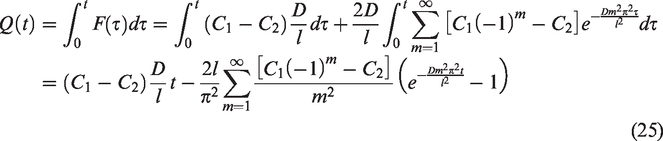
Therefore, Equation (25) becomes as follows

Q (t) = (C_{1} - C_{2}) \frac{D t}{l} + (\frac{l}{6} C_{1} + \frac{l}{3} C_{2}) \sum_{m = 1}^{\infty} (e^{- \frac{D m^{2} π^{2} t}{l^{2}}} - 1)

(28)

When t is very large, the exponential term in Equation (28) becomes small enough to ignore. Then $Q (t)$ is given by the following equation

Q (t) = (C_{1} - C_{2}) \frac{D}{l} t - \frac{l}{6} (C_{1} + 2 C_{2})

(29)

Thus, $Q (t)$ against $t$ tends to the linear equation. If $Q_{t} = 0$ in Equation (29), the intercept $L$ on the $t$ -axis is referred to as the time-lag and is given by the following equation

t = \frac{(C_{1} + 2 C_{2}) l^{2}}{6 (C_{1} - C_{2}) D} = L

(30)

Hence, if the boundary conditions are $C (0, t) = C_{1}$ and $C (l, t) = C_{2}$ and the initial condition is $C (x, 0) = C_{0} = 0$ , the diffusion coefficients can be obtained by the following equation

D = \frac{(C_{1} + 2 C_{2}) l^{2}}{6 (C_{1} - C_{2}) L}

(31)

Steady-state concentration distribution

In the case of diffusion using the film-roll method, the initial condition is $C (x, 0) = C_{0} = 0$ , $C_{1}$ in Equation (31) is the entrance surface concentration of the first layer, $C_{2}$ is the exit surface concentration of the first layer, and $l$ is the first layer thickness. Let ${\bar{C}}_{i}$ be the mean concentration of the $i th$ layer, $M$ be the total amount diffused from the first layer to the last layer, that is, $M = l \sum_{i = 1}^{n} \bar{C_{i}}$ , and $l_{v}$ be the total diffusion length under the steady-state condition.

Assuming a steady-state condition is set up for the sublimation diffusion of disperse dye to PET film by treating it at 190°C for 240 minutes, Figure 4 shows the profile of concentration–distance and the steady-state concentration distribution $v (x)$ .

Figure 4.

The profile of concentration–distance and the steady-state concentration distribution for the sublimation diffusion of disperse dye to polyethylene terephthalate film by treating it at 190°C for 240 minutes.

The linear function $v (x) = - (C_{1} x) / l_{v} + C_{1}$ was deduced from the assumption that the total amount $M$ is the area of a triangle, that is, $M = (C_{1} l_{v}) / 2$ , and $v (x)$ passes through the point of $\bar{C_{1}}$ at the center of the first layer. That is, $M$ , $C_{1}$ , and $\bar{C_{1}}$ at $x = 20 μ m$ are given by the following equations¹³

M = l \sum_{i = 1}^{n} \bar{C_{i}} = \frac{1}{2} C_{1} l_{v} ⟹ C_{1} = \frac{2}{l_{v}} M = \frac{2 l}{l_{v}} \sum_{i = 1}^{n} \bar{C_{i}} (32)

v (x) = - \frac{C_{1}}{l_{v}} x + C_{1} ⟹ \bar{C_{1}} = - \frac{C_{1}}{l_{v}} \times 20 + C_{1} (33)

Substituting $(2 M) / l_{v}$ for $C_{1}$ yields Equation (34). Thus $l_{v}$ , $C_{1}$ , and $C_{2}$ can be obtained by Equations (35) and (36)

\bar{C_{1}} = - \frac{40 M}{{l_{v}}^{2}} + \frac{2 M}{l_{v}} ⟹ {l_{v}}^{2} - \frac{2 M}{\bar{C_{1}}} l_{v} + \frac{40 M}{\bar{C_{1}}} = 0 (34)

a = \frac{2 M}{\bar{C_{1}}}, b = \frac{40 M}{\bar{C_{1}}} ⟹ l_{v} = \frac{a + \sqrt{a^{2} - 4 b}}{2} (μ m) (35)

C_{1} = \frac{2}{l_{v}} M (mg \cdot {cm}^{- 3}) and C_{2} = - \frac{C_{1}}{l_{v}} \times 40 + C_{1} (36)

The steady-state total diffusion length $l_{v}$ obtained by Equation (35) was $244.5 μ m$ . The boundary conditions of the steady-state first layer obtained by Equation (36) were $C_{1} = 84.9 mg \cdot {cm}^{- 3}$ and $C_{2} = 71.0 mg \cdot {cm}^{- 3}$ . The steady-state first layer amount $Q_{1}$ corresponding to the area of a trapezoid from $x = 0$ to $x = 40 μ m$ in Figure 4 was $0.3118 mg \cdot {cm}^{- 2}$ , which was obtained by $0.004 (C_{1} + C_{2}) / 2$ . The steady-state first layer-passed total amount $Q (t) = Q_{t}$ , which is the amount of dye passed through $x = 40 μ m$ and corresponds to the area of the right-hand triangle from $40$ to $244.5 μ m$ in Figure 4, was determined by subtracting $Q_{1}$ from $M$ , that is, $Q_{t} = M - Q_{1}$ .²³ The equation $Q_{t} = M - Q_{1}$ was also applied to the diffusion at less time than the time to reach a steady-state condition, that is, the diffusion at less time than 240 minutes, on the premise that the dye amount and the boundary conditions of the first layer for the diffusion at less time than 240 minutes were the same as those for the steady-state diffusion at 240 minutes.

Time-lag and diffusion coefficient

On treating at 190°C for various times, the mean dye concentration of the $i th$ layer, that is, ${\bar{C}}_{i}$ , and the steady-state first layer-passed total amount $Q_{t}$ obtained by $M = l \sum_{i = 1}^{8} \bar{C_{i}}$ and $Q_{t} = M - Q_{1}$ , where $Q_{1} = 0.3118 mg \cdot {cm}^{- 2}$ , are presented in Table 1.

Table 1.

Mean concentrations ${\bar{C}}_{i} (mg \cdot {cm}^{- 3})$ of film layers ( $i$ ) according to time at 190°C $(Q_{1} = 0.3118 mg \cdot {cm}^{- 2})$

${\bar{C}}_{i}$	30 min	60 min	120 min	180 min	240 min
${\bar{C}}_{1}$	38.3	59.3	76.9	77.7	78.0
${\bar{C}}_{2}$	16.6	26.0	43.1	53.1	61.2
${\bar{C}}_{3}$	5.8	12.6	22.7	33.5	44.8
${\bar{C}}_{4}$	–	5.0	12.8	21.5	30.7
${\bar{C}}_{5}$	–	–	7.8	13.1	21.0
${\bar{C}}_{6}$	–	–	3.9	9.2	12.5
${\bar{C}}_{7}$	–	–	–	5.4	7.5
${\bar{C}}_{8}$	–	–	–	3.4	3.9
$\sum_{i = 1}^{8} \bar{C_{i}}$	60.7	102.9	167.2	216.9	259.6
$M$	0.2428	0.4116	0.6688	0.8676	1.0384
$Q_{t}$	–0.0690	0.0998	0.3570	0.5558	0.7266

The value of $Q_{t}$ in Equation (29), which is deduced by integrating the rate of flow $F (t)$ at the face $x = l$ with respect to time and is obtained by the constants $C_{1}$ and $C_{2}$ , corresponds to $Q_{t}$ in Figure 4. The steady-state first layer-passed total amount $Q_{t}$ is the total amount of dye passed through the steady-state first layer in time $t$ on the premise that the first layer boundary conditions are constants, that is, $C (0, t) = C_{1}$ and $C (40 μ m, t) = C_{2}$ , regardless of its actual concentration–distance distribution. When plotting $Q_{t}$ against time to obtain the time-lag, for the diffusion of less time than the time to reach a steady-state condition, if the total amount diffused from the first layer to the last layer, that is, $M$ , is greater than the steady-state first layer amount $Q_{1}$ obtained by $v (x)$ , in other words if the values of $Q_{t}$ are positive, even though the concentration–distance distribution of the first layer dose not satisfy a steady-state condition and the values of $Q_{t}$ are small, the small values of $Q_{t}$ should not be discarded to reduce the ambiguity about the criteria for obtaining the time-lag and to increase the reliability of the time-lag obtained when $Q_{t}$ is zero. However, if $M$ is less than $Q_{1}$ , that is, if $Q_{t}$ is negative, the negative values of $Q_{t}$ are invalid because $C (0, t)$ and $C (40 μ m, t)$ are not constants. Thus, the plots of $Q_{t}$ against time were composed of all the positive values of $Q_{t}$ .

Figure 5 shows the plot of $Q_{t}$ against time for the diffusion at 190°C, excluding the negative value of $Q_{t}$ for 30 minutes, and its linear regression line. The linearity of Equation (29) for the diffusion at 190°C can be confirmed by the correlation coefficient ( $r = 0.99561$ ) of the linear regression line. The time-lag $L$ , which is the intercept on the time-axis when $Q_{t} = 0$ on $Q_{t} = 0.34653 t - 8.5$ , was $24.53$ minutes. The diffusion coefficient $D$ for the diffusion at 190°C was calculated by $C_{1}$ , $C_{2}$ , and $L$ according to Equation (31) as follows

D = \frac{(C_{1} + 2 C_{2}) l^{2}}{6 (C_{1} - C_{2}) L} = \frac{16.3 {\times 0.004}^{2}}{6 \times 24.53} = 1.7720 \times 10^{- 6} ({cm}^{2} \min^{- 1})

Figure 5.

Plot of $Q_{t}$ against time for diffusion at 190°C and its linear regression line.

Figure 6 shows the amount of each layer obtained from the mean dye concentration $\bar{C_{i}}$ for the sublimation diffusion of disperse dye to PET film by treating it at 180°C for 240 minutes and the steady-state concentration distribution $v (x)$ , which was deduced from the assumption that the approximate steady-state condition had been achieved at 180°C and 240 minutes. The total diffusion length $l_{v}$ under the steady-state obtained by Equation (35) was $170.1 μ m$ . The boundary concentrations $C (0, t) = C_{1}$ and $C (40 μ m, t) = C_{2}$ in the first layer were $57.1$ and $43.7 mg \cdot {cm}^{- 3}$ , respectively.

Figure 6.

On treating at 180°C for various times, the mean dye concentration of the $i th$ layer ${\bar{C}}_{i}$ and the steady-state first layer-passed total amount $Q_{t}$ obtained by $M = l \sum_{i = 1}^{5} \bar{C_{i}}$ and $Q_{t} = M - Q_{1}$ , where $Q_{1} = 0.2016 mg \cdot {cm}^{- 2}$ , are presented in Table 2.

Table 2.

Mean concentrations ${\bar{C}}_{i} (mg \cdot {cm}^{- 3})$ of film layers according to time at 180°C $(Q_{1} = 0.2016 mg \cdot {cm}^{- 2})$

${\bar{C}}_{i}$	30 min	60 min	120 min	180 min	240 min
${\bar{C}}_{1}$	25.9	34.9	45.4	49.5	50.4
${\bar{C}}_{2}$	6.7	13.9	21.0	28.5	34.0
${\bar{C}}_{3}$	-	3.9	10.5	13.8	20.2
${\bar{C}}_{4}$	-	-	5.4	7.5	11.6
${\bar{C}}_{5}$	-	-	-	3.5	5.2
$\sum_{i = 1}^{5} \bar{C_{i}}$	32.6	52.7	82.3	102.8	121.4
$M$	0.1304	0.2108	0.3292	0.4112	0.4856
$Q_{t}$	–0.0712	0.0092	0.1276	0.2096	0.2840

For the diffusion at 180°C, just like at 190°C, the value of $Q_{t}$ for 30 minutes of treatment time is negative and the values of $Q_{t}$ for treatment times greater than 60 minutes are positive. Thus, when plotting $Q_{t}$ against time, since $Q_{t}$ for 30 minutes is not valid, the negative value of $Q_{t}$ for 30 minutes is excluded.

Figure 7 shows the plot of $Q_{t}$ against time for the diffusion at 180°C and its linear regression line. The correlation coefficient ( $r = 0.99366$ ) of the linear regression line also substantiated the linearity of Equation (29) for the diffusion at 180°C. The time-lag $L$ calculated from $Q_{t} = 0.15107 t - 6.9$ was $45.67$ minutes. The diffusion coefficient $D$ was calculated as follows

D = \frac{(C_{1} + 2 C_{2}) l^{2}}{6 (C_{1} - C_{2}) L} = \frac{10.8 {\times 0.004}^{2}}{6 \times 45.67} = 6.3061 \times 10^{- 7} ({cm}^{2} \min^{- 1})

Figure 7.

Plot of $Q_{t}$ against time for the diffusion at 180°C and its linear regression line.

Figure 8 shows the graph of concentration–distance created from the mean dye concentration $\bar{C_{i}}$ for the diffusion at 170°C for 300 minutes and the steady-state concentration distribution $v (x)$ obtained on the premise that an approximate steady-state condition was achieved by the diffusion at 170°C for 300 minutes.

Figure 8.

The total diffusion length $l_{v}$ in the steady-state was $134.0 μ m$ . $C (0, t) = C_{1}$ and $C (40 μ m, t) = C_{2}$ in the first layer were $38.2$ and $26.8 mg \cdot {cm}^{- 3}$ respectively. On treating at 170°C for various times, the mean dye concentrations ${\bar{C}}_{i}$ and the steady-state first layer-passed total amount $Q_{t}$ obtained by $M = l \sum_{i = 1}^{4} \bar{C_{i}}$ and $Q_{t} = M - Q_{1}$ , where $Q_{1} = 0.1300 mg \cdot {cm}^{- 2}$ , are presented in Table 3.

Table 3.

Mean concentrations ${\bar{C}}_{i} (mg \cdot {cm}^{- 3})$ of film layers according to time at 170°C $(Q_{1} = 0.1300 mg \cdot {cm}^{- 2})$

${\bar{C}}_{i}$	60 min	120 min	180 min	240 min	300 min
${\bar{C}}_{1}$	21.5	26.9	30.8	32.2	32.5
${\bar{C}}_{2}$	7.8	10.2	11.6	16.6	20.0
${\bar{C}}_{3}$	-	3.3	4.7	8.3	11.1
${\bar{C}}_{4}$	-	-	1.8	3.6	5.8
$\sum_{i = 1}^{4} \bar{C_{i}}$	29.3	40.4	48.9	60.7	69.4
$M$	0.1172	0.1616	0.1956	0.2428	0.2776
$Q_{t}$	–0.0128	0.0316	0.0656	0.1128	0.1476

For the diffusion at 170°C, the value of $Q_{t}$ for 60 minutes of treatment time is negative and the values of $Q_{t}$ for treatment times greater than 120 minutes are positive. Thus, $Q_{t}$ for 60 minutes is excluded.

Figure 9 shows the plot of $Q_{t}$ against time for the diffusion at 170°C and its linear regression line. The linearity of Equation (29) for the diffusion at 170°C is also substantiated by the correlation coefficient ( $r = 0.9979$ ) of the linear regression line. The time-lag $L$ calculated from $Q_{t} = 0.06587 t - 4.892$ was $74.27$ minutes. The diffusion coefficient $D$ for the diffusion at 170°C was calculated as follows

D = \frac{(C_{1} + 2 C_{2}) l^{2}}{6 (C_{1} - C_{2}) L} = \frac{8.1 {\times 0.004}^{2}}{6 \times 74.27} = 2. 9083 \times 10^{- 7} ({cm}^{2} \min^{- 1})

Figure 9.

Plot of $Q_{t}$ against time for the diffusion at 170°C and its linear regression line.

Arrhenius plot

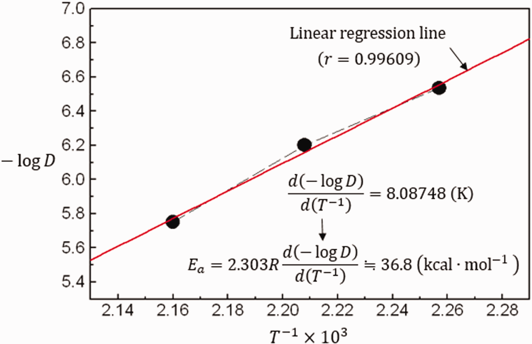
Table 4 presents the diffusion coefficients for the diffusion at 170°C, 180°C, and 190°C, and also presents the reciprocal of absolute temperatures $(T^{- 1})$ and negative common logarithms of the diffusion coefficients $(- \log D)$ to create the Arrhenius plot by Equation (2), where $E_{a}$ is the activation energy and $R$ is the gas constant (1.978 $cal \cdot K^{- 1} {mol}^{- 1}$ ).

Table 4.

Logarithms of $D$ for the Arrhenius plot

$T (°C)$	$T (K)$	$T^{- 1}$	$D$ (cm²·min^–1)	$- \log D$
190	463	2.160 $\times$ 10–3	$1.7720 \times 10^{- 6}$	$5.7515$
180	453	2.208 $\times$ 10–3	$6.3061 \times 10^{- 7}$	$6.2002$
170	443	2.257 $\times$ 10–3	$2. 9083 \times 10^{- 7}$	$6.5364$

Equation (2) is a linear function of $- \log D$ with respect to $T^{- 1}$ . The reliability of the diffusion coefficients obtained by the time-lag can be proved by the linearity of the Arrhenius plot. The activation energy, which indicates the sensitivity of the diffusion rate to temperature, is obtained by the slope of the linear regression line for the Arrhenius plot.

Figure 10 shows the Arrhenius plot and its linear regression line. The correlation coefficient of the linear regression line, which is a measure of the degree of linear relationship, was 0.99609, from which it was expected that the diffusion coefficients obtained by the time-lag were reasonable and reliable. The activation energy $E_{a}$ of diffusion calculated by Equation (2) was 36.8 $kcal \cdot {mol}^{- 1}$ .

Figure 10.

Arrhenius plot of diffusion coefficients and its linear regression line.

Comparison of three diffusion coefficient equations

In the previous two studies, the diffusion coefficients were obtained by two different equations. Equation (37) was deduced from a trigonometrical series and the diffusion coefficients $D^{F}$ were calculated by the surface concentration $C_{1}$ , the steady-state diffusion length $l_{v}$ , and the total amount diffused from the first layer to the last layer, that is, $l \sum_{i = 1}^{n} \bar{C_{i}}$ , in time $t$ to reach an approximate steady-state condition for the diffusion of 190°C $\times$ 240 minutes, 180°C $\times$ 240 minutes, and 170°C $\times$ 300 minutes¹³

D^{F} = \frac{l_{v}}{t} (\frac{l \sum_{i = 1}^{n} \bar{C_{i}}}{C_{1}} + \frac{l_{v}}{6})

(37)

Equation (38) was deduced from a series of error functions and the diffusion coefficients $D^{E}$ were calculated by obtaining $x / \sqrt{4 D t}$ of $erfc (x / \sqrt{4 D t})$ from $C_{x} / C_{1}$ of the concentration $C_{x}$ at distance $x$ to the surface concentration $C_{1}$ obtained by the concentration–distance profile for the diffusion in a specified time (180 minutes).¹² The profiles of $C_{x} / C_{1}$ versus $x / \sqrt{4 D t}$ were obtained from replacing $C_{x}$ with the mean dye concentration of the ith layer $(\bar{C_{i}})$

\frac{C_{x}}{C_{1}} = erfc (\frac{x}{\sqrt{4 D^{E} t}})

(38)

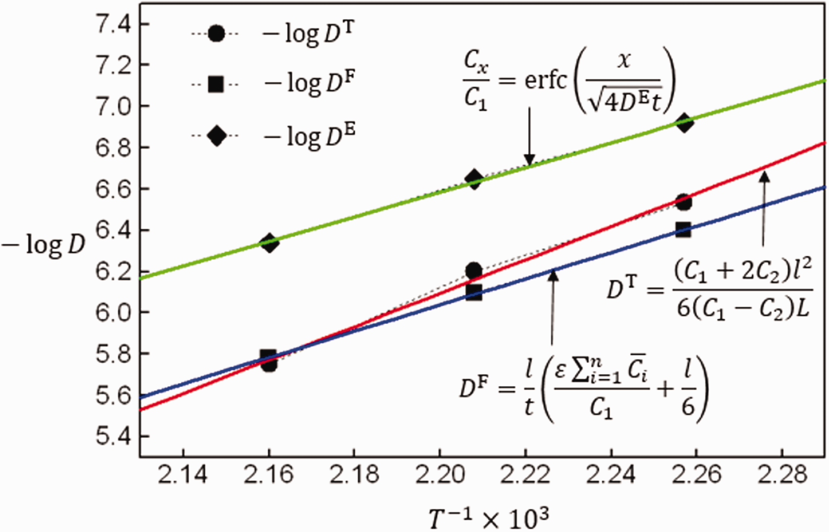
Let $D$ obtained by time-lag be denoted by $D^{T}$ to distinguish it from $D^{F}$ and $D^{E}$ . The values of $D^{T}$ , $D^{F}$ , and $D^{E}$ and their activation energies $(E_{a})$ are presented in Table 5. Their Arrhenius plots are shown in Figure 11.

Table 5.

Diffusion coefficients $(D^{T}, D^{F}, D^{E})$ , activation energies $(E_{a}),$ and correlation coefficients of linear regression lines for the Arrhenius plots $(r)$

$T (°C)$	$D^{T}$ (cm²·min^–1)	$D^{F}$ (cm²·min^–1)	$D^{E}$ (cm²·min^–1)
190	$1.772 \times 10^{- 6}$	$1.658 \times 10^{- 6}$	$4.655 \times 10^{- 7}$
180	$6.306 \times 10^{- 7}$	$8.037 \times 10^{- 7}$	$2.045 \times 10^{- 7}$
170	$2. 908 \times 10^{- 7}$	$3.991 \times 10^{- 7}$	$1.049 \times 10^{- 7}$
$E_{a}$	36.8 $kcal \cdot {mol}^{- 1}$	29.2 $kcal \cdot {mol}^{- 1}$	30.5 $kcal \cdot {mol}^{- 1}$
$r$	0.9961	0.9999	0.9978

Figure 11.

Linear regression lines for Arrhenius plots obtained by three diffusion coefficient equations.

The values of $D^{T}$ for the diffusion in various times (190°C $\times$ 60–240 minutes, 180°C $\times$ 60–240 minutes, and 170°C $\times$ 120–300 minutes) are similar to the values of $D^{F}$ for the diffusion in the specified time to reach an approximate steady-state (190°C $\times$ 240 minutes, 180°C $\times$ 240 minutes, and 170°C $\times$ 300 minutes). This is presumably because both the values of $D^{T}$ and $D^{F}$ are obtained by equations deduced from the same trigonometrical series. While the values of $D^{E}$ for the diffusion in 180 minutes under the non-steady-state are less than the values of $D^{T}$ and $D^{F}$ , it is presumed that the values of $D^{E}$ differ greatly from those of $D^{T}$ and $D^{F}$ because those of $D^{E}$ are obtained by an equation deduced from a series of error functions. On the other hand, the activation energy for $D^{T}$ is greater than those for $D^{F}$ and $D^{E}$ , which is presumed to be due to the fact that the values of $D^{T}$ are obtained for the diffusion in various times including the time to reach an approximate steady-state condition, while the values of $D^{F}$ and $D^{E}$ are obtained for the diffusion in a specified time. The correlation coefficients $(r)$ of the linear regression lines for the three Arrhenius plots were 0.9961–0.9999, which showed good linearity.

Conclusion

A method for determining the diffusion coefficient by time-lag using the film-roll method for the sublimation diffusion of disperse dye was proposed. PET film-roll coated with dye paste was treated at 170–190°C for various times. A solution consisting of the sum of a steady-state solution and a transient solution was obtained by the homogeneous boundary value problem from a trigonometrical series. Assuming a steady-state was set up over a long period, the boundary conditions of the first layer and the steady-state first layer amount were obtained from the steady-state concentration distribution. The steady-state first layer-passed total amount was obtained by subtracting the steady-state first layer amount from the total amount diffused from the first layer to the last layer. The time-lag was calculated from the linear regression line for the plot of the positive values of the steady-state first layer-passed total amount against time. The diffusion coefficient was calculated by the boundary conditions of the steady-state first layer and the time-lag. The correlation of the steady-state first layer-passed total amount against time was very linear. The reliability of the diffusion coefficients obtained by the time-lag was proved by the good linearity of the Arrhenius plot. The activation energy obtained was 36.8 kcal $\cdot$ mol⁻¹.

Footnotes

Declaration of conflicting interests

The author has no conflicts of interest to declare.

Funding

The author received no financial support for the research, authorship, and/or publication of this article.

ORCID iD

Geon Yong Park

References

Crank

The mathematics of diffusion. Oxford: Clarendon Press, 1975, p.47.

Vickerstaff

The physical chemistry of dyeing. London: Oliver and Boyd, 1954, p.125.

Sicardi

Manna

Banchero

Diffusion of disperse dyes in PET films during impregnation with a supercritical fluid. J Supercrit Fluid 2000; 17: 187–194.

Sicardi

Manna

Banchero

Comparison of dye diffusion in poly(ethylene terephthalate) films in the presence of a supercritical or aqueous solvent. Ind Eng Chem Res 2000; 39: 4707–4713.

Datyner

Delaney

Iijima

The interaction between acid dyes and nonionic surfactants and its effect on sorption and diffusion behavior part III: diffusion of dyes into polyamide 6 films. Text Res J 1973; 43: 48–53.

Shibusawa

Chigira

Dual-mode sorption of nonionic azo dyes by nylon 6. J Polym Sci Part B Polym Phys 1992; 30: 563–568.

Shibusawa

Diffusion of nonionic azo dyes in nylon 6. J Polym Sci Part B Polym Phys 1993; 31: 29–35.

Shibusawa

Diffusion of disperse dyes in nylon 6. Text Res J 1996; 66: 421–428.

Sekido

Matsui

Study on vat dyeing.

Sen-i Gakkaishi 1964; 20: 778–783.

10.

Park

GY.

Diffusion behaviors of disperse dye to PET film from print paste using film-roll method. Text Sci Eng 2017; 54: 125–130.

11.

Park

GY.

Diffusion coefficient for sublimation diffusion of disperse dye using error function. Int J Innov Tech Exploring Eng 2019; 8: 37–42.

12.

Park

GY.

Diffusion coefficient calculated by complementary error function for the sublimation diffusion of disperse dye. J Eng Fibers Fabrics 2019; 14: 1–9.

13.

Park

GY.

Study on calculation of diffusion coefficient for sublimation diffusion of disperse dye using Fourier series. Fiber Polym 2020; 21: 538–547.

14.

Madan

Khan

AH.

Determination of dye on textile fibers. Part I: disperse dye on polyethylene terephthalate. Text Res J 1978; 48: 481–486.

15.

Berg

HC.

Random walks in biology. Princeton: Princeton University, 1977, pp.17–18.

16.

Cain

Reynolds

AM.

Ordinary and partial differential equations. : Virginia Commonwealth University, Richmond, 2010, pp.313–315.

17.

Crank

The mathematics of diffusion. Oxford: Clarendon Press, 1975, pp.17–18.

18.

Heat equation. https://en.wikipedia.org/wiki/Heat equation (accessed 21 July 2020)

19.

Hildebrand

FB.

Advanced calculus for applications. : Englewood Cliffs: Prentice Hall Press, 1976, pp.214–215.

20.

Valeriy

Introduction to partial differential equations. Oulu: University of Oulu, 2011, pp.37–38.

21.

Crank

The mathematics of diffusion. Oxford: Clarendon Press, 1975, pp.49–51.

22.

Riemann zeta function. http://en.wikipedia.org/wiki/Riemann zeta function (accessed 11 August 2020).

23.

Jones

Leung

TSM.

Some fundamental aspects of transfer printing. J Soc Dye Colour 1974; 90: 286–290.