Simulation of fiber configuration in the sliver with the straightness and separation degree

Abstract

The fiber straightness and separation degree have the important influences on sliver properties. In this work, an innovative model of the fiber configuration considering straightness was presented and optimized by taking the fiber separation degree into account. The new developed model could simulate fiber assemblies and all kinds of separated fibers, including hooked fibers and straight fibers. Furthermore, some thin and thick segments were presented in the optimized simulated sliver with consideration of the fiber separation degree, and the simulated sliver irregularities were close to the actual ones. The relative errors between tested sliver irregularities and simulated ones were reduced from around 80% to less than 30%. Besides, the influence of each fiber parameter on the sliver irregularity could be drawn from the novel model of fiber configuration in the sliver, which verified the necessity of the applications of the straightness and separation degree. Therefore, it could be concluded that the introduction of the fiber straightness and the consideration of the fiber separation degree made more accurate and reasonable simulation of the fiber configuration in the sliver. Moreover, the straightening process of the hooked fibers and the random combination between thick fragments and thin fragments during the drawing simulation could be realized based on this model in the future.

Keywords

Fiber configuration sliver irregularity straightness separation degree fiber parameter

Quantifying sliver irregularity has been the objective of considerable theoretical work in the field of evaluating sliver quality.^1–17 Spencer-Smith and Todd¹⁰ firstly made efforts to study sliver evenness by postulating that the number of fibers in the sliver cross-section follows the Poisson distribution. Martindale⁹ devised a classical calculation method of yarn limit irregularity based on the same assumption. Later, it was confirmed that the distribution of fiber heads in the sliver was a major influence factor on the sliver irregularity with the model of fiber arrangement.^1,11 Later, Cherkassky^2,3 introduced a discrete-event model of one-dimensional fibrous material into the simulation of the fiber arrangement in the sliver to calculate the sliver evenness. However, the sliver irregularity calculated in the foregoing models of fiber arrangement was expressed as the irregularity of the fiber number in the sliver cross-section, which was out of line with the tested sliver irregularity in the short-term.

Afterwards, the fiber length and its distribution were taken into consideration to calculate the sliver irregularity in the short-term based on the model of fiber arrangement in the sliver.^6,18,19 Besides, the irregularity of the total weight of fibers within each sliver subsection was obtained by applying the fiber fineness distribution in the sliver simulation.^7,20 Notwithstanding all this, the assumption that fibers were completely separated and straight along the sliver axis in these methods leads to far fewer simulated sliver irregularities than actual ones. Actually, there were some hooked fibers in the fibrous-flux (sliver, roving, and yarn); for instance, in the card sliver, more than 70% of fibers were hooked.^4,15,21–25 Thereby, Yang et al.¹⁴ introduced fiber straightness into the simulation of the fiber arrangement in the sliver based on the model with straight fibers^6,7 In their models, the straightness of every fiber was assumed to be identical. However, the straightness of each fiber was different, and the straightness of about 30% fibers was lower than 0.5 in the practical sliver.¹⁵ Besides, fibers were not fully separately arranged in the specific sliver.^8,12,17 Many experimental studies have been made and revealed that 30–50% of fibers in the card sliver were not separated fibers, but rather fiber assemblies.^26–28

There is no doubt that all the studies have contributed to analyzing the fiber configuration in the sliver (FCS). Nonetheless, the sliver irregularities calculated by previous models of fiber configuration are still far fewer than the measured ones. Therefore, in this study, a new model of FCS based on hook morphology with different straightness and separation degree was designed to achieve the goal of optimizing the mode of the straight fiber arrangement in the sliver and improving the prediction precision of sliver irregularity. The object of the work presented here was to simulate the fiber in a completely random configuration in the sliver taking the fiber straightness unevenness into consideration firstly. Secondly, the fiber incompletely random configuration in the sliver was developed by applying the fiber separation degree in the simulation to accomplish the refinement. Ultimately, the fiber configuration could be displayed more precisely, and the prediction of sliver irregularities could be greatly improved. In this work, the FCS model was run by MATLAB software.

Assumptions of the model

It was certain that the position distribution of the fiber heads makes a considerable contribution to the FCS.^16,29 According to previous researches,^16,29 the positions of fiber heads in a given sliver segment were randomly simulated based on that the positions of fiber heads following the uniform distribution along the sliver axis in this model. In regard to the model of FCS with fiber straightness, fiber heads are regarded as the heads of the separated fibers in the sliver. In regard to the model of FCS with the fiber separation degree, fiber heads were regarded as the heads of the separated fibers and the fiber assemblies in the sliver. Considering the fiber straightness and fiber separation degree, two assumptions in this study were made to simplify the analysis of the sliver irregularity as follows:
the hooked parts and body parts of fibers are parallel along the sliver axis;

the position of each fiber is independent of its corresponding length, fineness, straightness, and separation degree.

Model of the fiber configuration in the sliver

As illustrated in Figure 1, the module “Head1” generated the number of fiber heads in a sliver segment based on the geometrical parameters of the fiber and the sliver. The consecutive module “Head2” simulated the positions of the fiber heads in the given sliver segment, which meet the uniform distribution. The module “Fiber” is the virtual simulation of the FCS. The positions of fibers would be obtained from the fiber length and fiber straightness when the body heads of the fibers had been confirmed. Generally, along the direction of sliver movement, fiber shapes in the sliver were divided into five kinds: the leading hooked fiber, trailing hooked fiber, hooked fiber at both ends, other hooked fiber, and straight fiber.^{4,14,15,21,22} Lastly, the module “Irregularity” calculated the sliver unevenness, which is the coefficient of variation of sliver weights in the short-term. The fiber lengths and their fineness of every sliver in the short-term were recorded to calculate the fiber weights of every short fragment. The weights of fibers are equal to the product of the fiber lengths and their fineness in the sliver in the short-term. It is well known that the short-term lengths used in measuring the irregularity of yarn, rovings, and slivers are different, for example, the short-term length of yarn is 8 mm, but it is 12 mm for slivers. Hence, what is calculated in this paper was the sliver irregularity of 12 mm.

Simulation of the fiber configuration in the sliver with the fiber straightness

Modeling

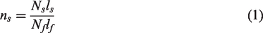
When the separation degree of fibers is not considered in the simulation of the FCS with the fiber straightness, every fiber is completely separated so that the fiber number in the sliver segment, n_s, is as follows:
$n_{s} = \frac{N_{s} l_{s}}{N_{f} l_{f}}$
(1)
where l_s denotes the sliver length; l_f denotes the mean fiber length; N_s denotes the sliver linear density; and N_f denotes the mean fiber fineness. Hence, the geometrical parameters of the fiber and sliver in the model of the FCS with the fiber straightness, including the length and fineness, are what needs to be input into the module “Head1.” In this model, the simulation of “Head2” can be obtained under the following condition: the head positions of the body parts of fibers submit to the uniform distribution in the sliver segment.

In order to describe the configuration of the hooked fibers, the fiber straightness, η, which is equal to the ratio of the hook length to the body length of hooked fiber, was applied in the simulation of the FCS. In the consecutive simulation of the FCS with the fiber straightness, straightness was assumed to meet the normal distribution, that is, η ∼ (η_f, $σ_{η}^{2}$ ), where η_f is the mean straightness and σ_η is the standard deviation (SD) of straightness. In Zhang’s study,¹⁵ it was verified to be reasonable that the distribution of straightness meets the normal distribution. During the simulation process of “Fiber,” when the fiber straightness η_i ≥ 0.5, the fiber was assumed to be bent one time; on the other hand, if η_i < 0.5, the fiber was assumed to be bent two times, and the hook parts had the same length. Here, i is the fiber serial number. The fibers in the sliver were classified into five groups^{4,14,15,21,22}: the leading hooked fiber, trailing hooked fiber, hooked fiber at both ends, other hooked fiber, and straight fiber. The actual and simulated fiber shapes in the sliver are shown in Table 1.

Table 1.
The actual and simulated fiber shapes in the sliver

Fiber shapes Straightness Leading hooked fiber Trailing hooked fiber Hooked fiber at both ends Other hooked fiber Straight fiber

Actual shapes η_i ≥ 0.5

η_i < 0.5

Simulated shapes η_i ≥ 0.5

η_i < 0.5

Sliver movement direction

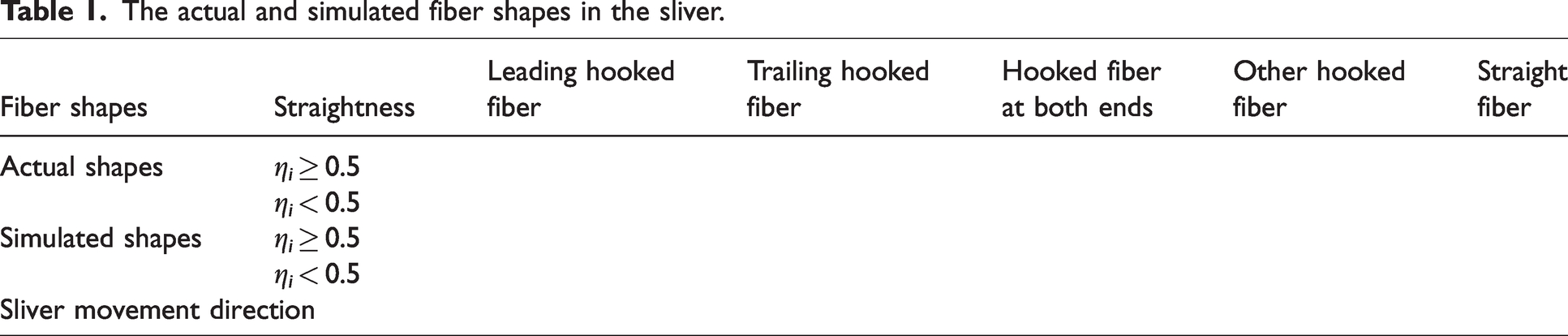
As indicated in Table 1, if η_i ≥ 0.5, the hook parts of the leading hooked fiber, trailing hooked fiber, and hooked fiber at both ends are represented by only a heavy line and the hook part of the other hooked fiber is represented by two heavy lines. On the other hand, when η_i < 0.5, the lines of the hook parts of the leading hooked fiber, trailing hooked fiber, and hooked fiber at both ends are bold three times and the line of hook part of the other hooked fiber are bold four times. Furthermore, it was noted that the front-hook part of the other hooked fiber was stochastically generated from 0 to the hook length of the fiber, and the back-hook part equaled the rest of the hook length out of the front-hook part. Moreover, the hook length, l_hi, and the body length, l_bi, could be calculated by the fiber length, l_i, and its corresponding straightness, η_i, as follows:
$l_{h i} = l_{i} (1 - η_{i})$
(2)

$l_{b i} = l_{i} η {}_{i}$
(3)

Consequently, the FCS is shown in Figure 2 in light of the positions of the fiber heads, fiber fineness, and fiber straightness. As shown in Figure 2, the black line is defined as the body part of fiber and the blue line is defined as the overlap between the body part and the hook part of the fiber in the simulated sliver. During the calculation process of sliver irregularity, in order to ensure the integrity of the sliver segment, the sliver segment with the maximal fiber length, l_max, should be expelled from the sliver body, because sliver formation in this part is incomplete, as shown in Figure 2. Then the sliver irregularity was calculated as the coefficient of variation of sliver weights with short-term length, Δl.

Figure 1.
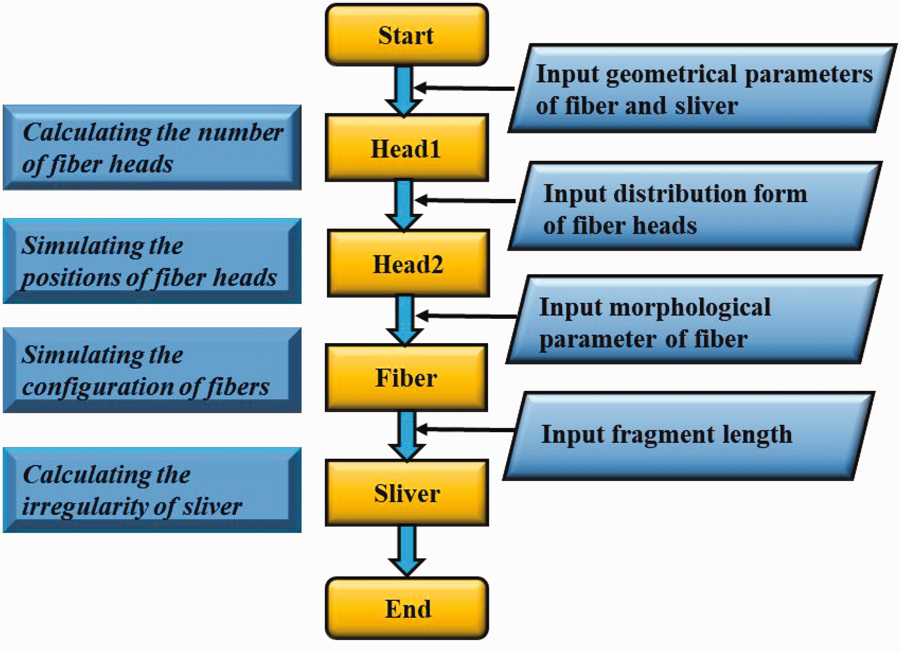
Flow chart of the model of the fiber configuration in the sliver.

Figure 2.
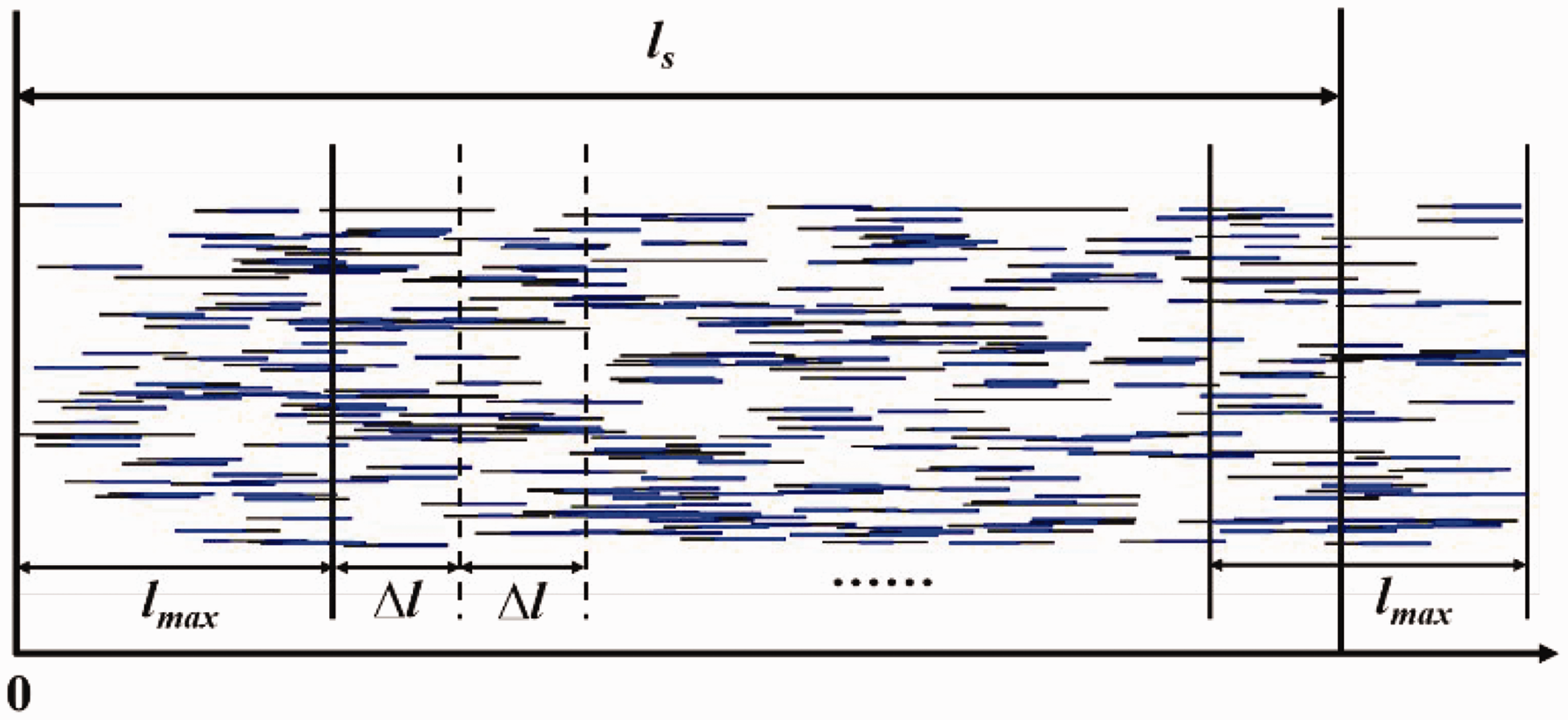
Schematic diagram of the fiber configuration in the sliver with the fiber straightness (color online only).

Results and discussion

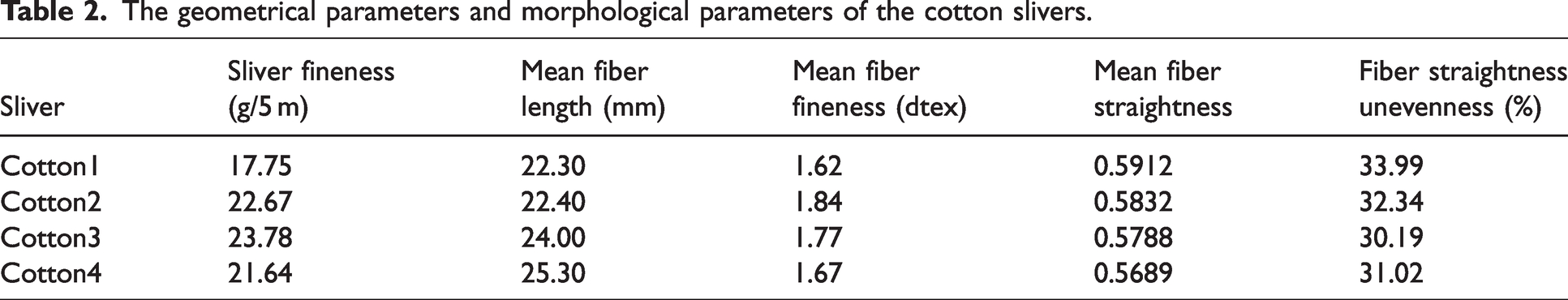
It had been proved that the geometrical parameters have a great influence on yarn irregularity when fibers are assumed to be straight during the fiber arrangement simulation.^6,7 To verify the rationality of the FCS with fiber straightness, the geometrical parameters and morphological parameters of the four kinds of cotton sliver shown in Tables 2 and 3 were input into the simulation program. These cotton slivers were provided by Long Run Textile Co., Ltd. The straightness and the proportions of different morphological fibers were tested by the tracer-fiber technique. Concretely, the cotton net containing tracer fibers was fed into a blowing carding unit to form the carding sliver. Then the species of the tracer fibers in the carding sliver were recorded. Besides, the lengths of the hook part and body part of every hooked fiber were measured to calculate the straightness. Every 100 tracer fibers were regarded as one set of experimental data. Meanwhile, the straightness of every fiber could be acquired by the length of the hook section and the body section for every fiber. The percent of different fibers and straightness were calculated as the mean value of 10 sets of experimental data. The mean and SD of the proportions of different morphological fibers are shown in Table 3. The fiber length distributions and the fiber fineness distributions were tested by an USTER AFIS Pro, and are specified in Figure 3. For the goal to future explore the effect of the morphological parameters on the sliver irregularity with the hooked fiber configuration, slivers without straightness, with mean straightness and with straightness distribution, were simulated.

Table 2.
The geometrical parameters and morphological parameters of the cotton slivers

Sliver Sliver fineness (g/5 m) Mean fiber length (mm) Mean fiber fineness (dtex) Mean fiber straightness Fiber straightness unevenness (%)

Cotton1 17.75 22.30 1.62 0.5912 33.99

Cotton2 22.67 22.40 1.84 0.5832 32.34

Cotton3 23.78 24.00 1.77 0.5788 30.19

Cotton4 21.64 25.30 1.67 0.5689 31.02

Table 3.
The proportions of different morphological fibers (%)

Sliver Leading hooked fiber
Trailing hooked fiber
Hooked fiber at both ends
Other hooked fiber
Straight fiber

Mean SD Mean SD Mean SD Mean SD Mean SD

Cotton1 10 1.14 54 3.96 17 3.27 8 1.14 11 1.82

Cotton2 8 1.08 56 3.14 11 3.45 10 1.42 15 2.02

Cotton3 10 1.26 47 3.42 18 2.88 10 1.56 15 1.88

Cotton4 11 1.24 52 3.86 14 3.28 9 2.04 14 1.50

Figure 3.
Distributions of fiber lengths and fiber fineness: (a) fiber lengths of Cotton1; (b) fiber fineness of Cotton1; (c) fiber lengths of Cotton2; (d) fiber fineness of Cotton2; (e) fiber lengths of Cotton3; (f) fiber fineness of Cotton3; (g) fiber lengths of Cotton4; (h) fiber fineness of Cotton4.

As is evident from Figure 4, the simulated irregularities without straightness, with mean straightness, and with straightness unevenness are observed to be compared with the tested result. It turns out that the sliver irregularities calculated by simulating the random fiber configuration taking the fiber straightness into account are all greater than the results obtained by the simulation based on the straight fiber configuration. This can be explained by the fact that more crimp fibers in the sliver will deteriorate the sliver evenness. Therefore, it can be drawn from the simulated sliver irregularity that it is reasonable to simulate the fiber configuration with the fiber straightness.

Figure 4.
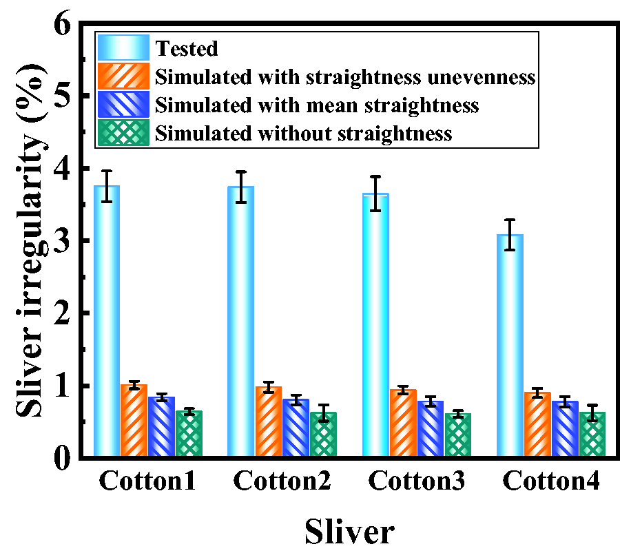
Simulated sliver irregularities without straightness, with mean straightness, with straightness unevenness, and tested sliver irregularities.

Moreover, as depicted in Figure 4, the sliver irregularities simulated with identical fiber straightness are distinctly lower than the results calculated from the simulation considering the fiber straightness distribution. This is largely due to the greater variability of the weight of the sliver in the short-term in the simulated sliver taking the fiber straightness distribution. The result indicates that it is necessary to introduce the fiber straightness distribution into the fiber configuration simulation. It can be inferred that it provides more reasonable description of the FCS when the fiber straightness distribution is considered.

However, all the simulated results are greatly lower than the tested ones. Not only the fiber straightness but also the fiber separation degree will be influenced by the fore-spinning process before the drawing procedure. Consequently, the degree of fiber separation is also one of the critical factors influencing the sliver irregularity. As is reported in previous research,^2,27 the fibers in the sliver are not fully separated. Therefore, the fiber separation degree should be applied in enhancing the simulated accuracy of the FCS.

Simulation of the fiber configuration in the sliver with the fiber separation degree

Modeling

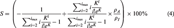
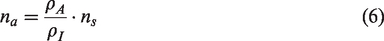
During the simulation of the FCS with the fiber separation degree, the application of the fiber separation degree was reflected in the processes of “Head1” and “Head2” whilst the other steps were simulated by the same method. In “Head1,” the numbers of all the fibers, n_s, separated fibers, n₁, and fiber assemblies, n_a(i ≤ i ≤ i_max) were firstly calculated according to the separation degree, S, as expressed in Equation (4)¹²:
$S = (- \frac{1}{\sum_{i = 2}^{i_{\max}} i \frac{K^{i}}{i! e^{K}} - 1} + \frac{\sum_{i = 2}^{i_{\max}} i \frac{K^{i}}{i! e^{K}}}{\sum_{i = 2}^{i_{\max}} i \frac{K^{i}}{i! e^{K}} - 1} \times \frac{ρ_{A}}{ρ_{I}}) \times 100 %$
(4)
where i represents the fiber number in the assembly; K represents the mean value of the Poisson distribution; i_max is 9 and K is 5 in the card cotton sliver^26–28; ρ_I represents the volume density of the ideal sliver; ρ_A represents the volume density of the actual sliver. During the testing process, the ideal sliver is the sliver combed completely, where the fibers are fully separated. Consequently, S can be acquired by testing from ρ_I and ρ_A, which are respectively measured as the weight of completely separated fibers and of fibers of the actual sliver in a unit volume. According to a previous study,¹² n₁ and n_a can be calculated as follows:
$n_{1} = S \cdot n_{s}$
(5)

$n_{a} = \frac{ρ_{A}}{ρ_{I}} \cdot n_{s}$
(6)

Then, based on the calculated n₁, n_a (1 ≤ i ≤ i_max), and n_s, the fiber numbers in the assemblies (2 ≤ i ≤ i_max) were arbitrarily simulated by the Poisson distribution in “Head1.”

Continuously, the head positions of the body part of the fiber assemblies (1 ≤ i ≤ i_max) could be randomly simulated along the sliver axis in the light of the uniform distribution in “Head2.” In the assemblies (2 ≤ i ≤ i_max), the head location of the body part of every fiber could be characterized by the head position of the corresponding assembly. Likewise, the positions of the body part and hook part could be simulated by the method in the “Fiber” module of the FCS simulation with the fiber straightness. Lastly, the simulated sliver segment considering the degree of fiber separation is as presented in Figure 5. As described in Figure 5, the green bold line is defined as the fiber assembly (2 ≤ i ≤ i_max). Likewise, the sliver irregularity was calculated as the coefficient of variation of sliver weights with short-term length, Δl, as shown in Figure 5. The sliver segment with the maximal fiber length, l_max, was expelled from the sliver body in order to ensure the integrity of the sliver segment during the calculation process of sliver irregularity. Moreover, the application of the fiber separation degree could accomplish the simulation of the configuration of thick fragments and thin fragments in the sliver, which is line with the actual sliver arrangement, as displayed in Figure 5.

Figure 5.
Schematic diagram of the fiber configuration in the sliver with the fiber separation degree (color online only).

Results and discussion

In order to analyze the influence of the fiber separation degree, the fiber configurations of four kinds of cotton slivers were simulated based on the model of the FCS with the fiber separation degree. As shown in Figure 6, the simulated irregularities with the fiber separation degree are much larger than the completely random simulated ones without the fiber separation degree. Moreover, the relative errors between the tested irregularities and the simulated ones are around 70% when the fibers in the sliver are assumed to be completely separated with hooked fibers (M2), but are only about 10% higher than the relative errors between the tested irregularities and the simulated ones when the fibers in the sliver are assumed to be completely separated with straight fibers (M1), as illustrated in Table 4. The application of the fiber separation degree can accomplish the simulation of the configuration of thick fragments and thin fragments in the sliver, which can cause a greater variability of the weight of the sliver in the short-term in the simulated sliver. Consequently, the relative error between the tested irregularities and the simulated ones decline to be lower than 30% if the separation degree is taken into consideration (M3). The prediction accuracy of sliver irregularity is approximately enhanced by 40%, which is in accordance with the fact that the fiber assembly will deteriorate the sliver evenness in the actual spinning process.^11,14,24 Therefore, it can be drawn from the results that the simulation considering the fiber separation degree is more suitable to describe the cotton FCS and predict the sliver irregularity.

Figure 6.
Simulated sliver irregularities with and without η and S and tested sliver irregularities.

Table 4.
The separation degree and relative errors between tested and simulated sliver irregularities

Sliver Separation degree S (%) Relative error between T and M3 (%) Relative error between T and M2 (%) Relative error between T and M1 (%)

Cotton1 62.10 27.20 73.07 82.85

Cotton2 67.03 29.04 73.80 83.36

Cotton3 61.07 27.70 74.25 83.28

Cotton4 64.96 16.78 70.78 79.75

Influences of fiber parameters on the sliver irregularity

Based on the model of the FCS, sliver irregularity can be calculated from the simulated fiber configuration. Thus, in order to compare the influence of every parameter on the sliver irregularity, the sliver irregularities with different fiber parameters based on the simulation of the FCS are shown in Figure 7. The fiber parameters included the mean fiber length, fiber length distribution, mean fiber fineness, fiber fineness distribution, mean fiber straightness, fiber straightness distribution, and fiber separation degree. During the simulation, every fiber parameter was increased or decreased by 5% according to the benchmark parameter. Besides, in order to analyze the effects of the fiber length distribution and the fiber fineness distribution, the length and fineness of each fiber were all simulated according to the normal distribution. Therefore, the influences of the fiber length distribution, fiber fineness distribution, and the straightness distribution could be expressed by the influences of the fiber length unevenness, fiber fineness unevenness, and straightness unevenness. The fiber length unevenness and fiber fineness unevenness of the four cotton slivers are shown in Table 5.

Figure 7.
Comparation of influences of the fiber parameters on the sliver irregularity: (a) Cotton1; (b) Cotton2; (c) Cotton3; (d) Cotton4.

Table 5.
Fiber length unevenness and fiber fineness unevenness of four cotton slivers

Sliver Fiber length unevenness CV_l (%) Fiber fineness unevenness CV_N (%)

Cotton1 38.25 36.41

Cotton2 37.22 39.10

Cotton3 39.10 38.79

Cotton4 37.40 37.88

As seen from the description in Figure 7, the sliver evenness almost remains constant with the increasement of CV_l. It is verified that the fiber length unevenness has little effect on the sliver irregularity. As the mean fiber length increases, the sliver evenness gradually improves. Likewise, the sliver irregularity declines with the increasing of η_f and S. In contrast, as the mean fiber fineness increases, the sliver gradually deteriorates. The sliver irregularity also shows an increasing trend as CV_N grows and CV_η grows. Besides, it can be drawn from the transition rates of sliver irregularity with the fiber parameters shown in Table 6 that the order of influence of each fiber parameter on the sliver irregularity is S > η_f > N_f > l_f > CV_η > CV_N > CV_l. The comparison results prove the necessity of introducing the fiber straightness and the fiber separation degree into the simulation of the FCS.

Table 6.
Transition rates of sliver irregularity with the fiber parameters

Sliver l_f (mm) CV_l (%) N_f (dtex) CV_N (%) η_f (%) CV_η (%) S (%)

Cotton1 1.14 0.07 1.31 0.43 1.01 0.73 2.91

Cotton2 1.10 0.05 1.21 0.54 0.83 0.72 2.64

Cotton3 1.04 0.03 1.25 0.49 0.88 0.77 2.07

Cotton4 1.12 0.05 1.48 0.53 0.99 0.84 2.41

Conclusion

Based on the previous model of the random FCS with straight fiber, the hook morphology with different straightness was taken into consideration in this work firstly. The application of the straightness realized the configuration simulation of five fiber shapes, including four kinds of hooked fibers and straight fiber, in the simulated sliver according to the proportion of different morphological fibers. The simulations of the FCS with straightness made for larger simulated sliver irregularities than those simulated with straight fiber. In particular, the sliver irregularities simulated considering the fiber straightness distribution were proved to be evidently larger than the simulated results with the identical fiber straightness. The application of fiber straightness provided significant influence on the fiber configuration and improved the predication accuracy of the sliver irregularity.

Besides, another feature worth mentioning in this present paper was the optimization considering the fiber separation degree in simulating the incomplete random FCS. The fiber configuration with thin and thick segments was accomplished by the simulation of the fiber assembly, which was in accordance with the actual sliver configuration. Therefore, the simulations of the FCS with the fiber separation degree were proved to be more accurate and effective to explore the FCS and predict the sliver irregularity.

In addition, the comparison of the influences of the fiber parameters on the sliver irregularity verified again that the introductions of fiber straightness and fiber separation degree were absolutely necessary. The fiber configuration model with the fiber straightness and the fiber separation degree can provide the foundation of the later drawing simulation. The straightening process of the hooked fibers can be realized in the future drafting simulation. The random combination during the drawing simulation between thick fragments and thin fragments can be accomplished in the future. Thus, the fiber motion during the drawing process can be concretely and figuratively simulated and the sliver quality after the drawing process can be accurately predicted with the aim of saving raw material costs and time costs.

Sliver	Sliver fineness (g/5 m)	Mean fiber length (mm)	Mean fiber fineness (dtex)	Mean fiber straightness	Fiber straightness unevenness (%)
Cotton1	17.75	22.30	1.62	0.5912	33.99
Cotton2	22.67	22.40	1.84	0.5832	32.34
Cotton3	23.78	24.00	1.77	0.5788	30.19
Cotton4	21.64	25.30	1.67	0.5689	31.02

Sliver	Leading hooked fiber	Trailing hooked fiber	Hooked fiber at both ends	Other hooked fiber	Straight fiber
Cotton1	10	1.14	54	3.96	17	3.27	8	1.14	11	1.82
Cotton2	8	1.08	56	3.14	11	3.45	10	1.42	15	2.02
Cotton3	10	1.26	47	3.42	18	2.88	10	1.56	15	1.88
Cotton4	11	1.24	52	3.86	14	3.28	9	2.04	14	1.50

Sliver	Separation degree S (%)	Relative error between T and M3 (%)	Relative error between T and M2 (%)	Relative error between T and M1 (%)
Cotton1	62.10	27.20	73.07	82.85
Cotton2	67.03	29.04	73.80	83.36
Cotton3	61.07	27.70	74.25	83.28
Cotton4	64.96	16.78	70.78	79.75

Sliver	Fiber length unevenness CV_l (%)	Fiber fineness unevenness CV_N (%)
Cotton1	38.25	36.41
Cotton2	37.22	39.10
Cotton3	39.10	38.79
Cotton4	37.40	37.88

Sliver	l_f (mm)	CV_l (%)	N_f (dtex)	CV_N (%)	η_f (%)	CV_η (%)	S (%)
Cotton1	1.14	0.07	1.31	0.43	1.01	0.73	2.91
Cotton2	1.10	0.05	1.21	0.54	0.83	0.72	2.64
Cotton3	1.04	0.03	1.25	0.49	0.88	0.77	2.07
Cotton4	1.12	0.05	1.48	0.53	0.99	0.84	2.41

Footnotes

Declaration of conflicting interests

The author(s) declared no potential conflicts of interest with respect to the research, authorship, and/or publication of this article.

Funding

The author(s) disclosed receipt of the following financial support for the research, authorship, and/or publication of this article: This work was supported by the Natural Science Foundation of Shandong Province (ZR2022QE164) and the Innovation and Entrepreneurship Training Program for College Students of Shandong Province (S202212332014).

ORCID iD

Na Sun

References

Brown

NG.

Statistics for the number of fiber ends in a segment of a random assembly of aligned fibers. Text Res J 1985; 55: 206–210.

Cherkassky

Neural network meta‐model of fibrous materials based on discrete‐event simulation. Part 1: discrete‐event simulation model of one‐dimensional fibrous material. J Text Inst 2011; 102: 442–454.

Cherkassky

Discrete-event simulation model of roll‐drafting process. J Text Inst 2011; 102: 1044–1058.

Garde

Wakankar

Bhaduri

SN.

Fiber configuration in sliver and roving and its effect on yarn quality. Text Res J 1961; 31: 1026–1036.

Huang

Zhang

Zhong

et al. The behavior between fluid and structure from coupling system of bile, bile duct, and polydioxanone biliary stent: a numerical method. Med Eng Phys 2023; 113: 103966.

Jiang

Kuang

et al. Simulation on fiber random arrangement in the yarn. J Text Inst 2014; 105: 1312–1318.

Jiang

Kuang

Yang

et al. Simulation on fiber random arrangement in the yarn part II: joint effect of fiber length and fineness distribution. J Text Inst 2016; 108: 347–352.

Liu

Dong

Chen

et al. Biodegradable and cytocompatible hydrogel coating with antibacterial activity for the prevention of implant-associated infection. ACS Appl Mater Interfaces 2023; 15: 11507–11519.

Martindale

JG.

A new method of measuring the irregularity of yarns with some observations on the origin of irregularities in worsted slivers and yarns. J Text Inst Trans 1945; 36: 35–47.

10.

Spencer-Smith

Todd

HAC.

A time series met within textile research. J R Stat Soc 1941; 7: 131–135.

11.

Suh

MW.

Probabilistic assessment of irregularity in random fiber arrays-effect of fiber length distribution on “variance-length curve”. Text Res J 1976; 46: 291–298.

12.

Sun

Simulation of fiber arrangement in the sliver with fiber separation degree. J Nat Fibers 2022; 19: 1419–1427.

13.

Yan

Zhu

A new approach to theoretical yarn unevenness: a binomial distribution model. J Text Inst 2010; 101: 753–757.

14.

Yang

Shen

Zhang

A study of fiber configuration in sliver fiber arrangement and its influence on sliver limit irregularity. Text Res J 2019; 89: 4799–4807.

15.

Zhang

Effect of fiber shape and arrangement on yarn or sliver irregularity. MS Thesis, Donghua University, Shanghai, 2016.

16.

Zhang

Jiang

et al. Distribution of fiber left ends in card sliver. J Text Res 2016; 37: 28–31.

17.

Zhang

Wang

Fan

et al. Doped CNC-Na2CO3 reinforcing alginate bio-based fiber as fire-safety composite applied in the household textile. Compos Commun 2023; 37: 101435.

18.

Yan

Stochastic simulation of yarn unevenness. J Text Res 2012; 33: 33–38.

19.

Yan

A joint influence of the distributions of fiber length and fineness on the strength efficiency of the fibers in yarn. Fibers Polym 2007; 18: 309–312.

20.

Qian

et al. Simulation study on effect of drafting on sliver unevenness. J Text Res 2021; 42: 85–90.

21.

Morton

Summers

RJ.

Fibre arrangement in card slivers. J Text Inst Proc 1949; 40: 106–116.

22.

Morton

Yen

KC.

Fibre arrangement in cotton slivers and laps. J Text Inst Trans 1952; 43: 463–472.

23.

Wakankar

Bhaduri

Ramaswamy

et al. Some studies on the formation of hooks in carding. Text Res J 1961; 31: 931–940.

24.

Ghosh

Bhaduri

SN.

Dependence of hook removal at drawing on some drafting parameters. Text Res J 1962; 32: 864–866.

25.

Fei

Study on hook orientation and fiber straightness. Text Technol Proc 2009; 2: 20–23 + 29.

26.

Zhang

Yan

Study on evaluating carding quality of carding roller. J Text Res 1987; 8: 517–522.

27.

Gao

Study on the fiber separation degree by weight method. J Text Res 1989; 10: 9–11.

28.

Zhao

Shen

Study on evaluating carding quality by measuring fiber separation degree. Cotton Text Technol 1989; 17: 516–520.

29.

Zhang

Jiang

et al. Mathematical modeling of ideal yarn based on Poisson process and the analysis of yarn unevenness. Math Pract Theor 2017; 47: 229–234.

Fiber shapes	Straightness	Leading hooked fiber	Trailing hooked fiber	Hooked fiber at both ends	Other hooked fiber	Straight fiber
Actual shapes	η_i ≥ 0.5
Actual shapes	η_i < 0.5
Simulated shapes	η_i ≥ 0.5
Simulated shapes	η_i < 0.5
Sliver movement direction

Sliver	Leading hooked fiber		Trailing hooked fiber		Hooked fiber at both ends		Other hooked fiber		Straight fiber
Sliver	Mean	SD	Mean	SD	Mean	SD	Mean	SD	Mean	SD
Cotton1	10	1.14	54	3.96	17	3.27	8	1.14	11	1.82
Cotton2	8	1.08	56	3.14	11	3.45	10	1.42	15	2.02
Cotton3	10	1.26	47	3.42	18	2.88	10	1.56	15	1.88
Cotton4	11	1.24	52	3.86	14	3.28	9	2.04	14	1.50