
Abstract
This paper utilises two politically determined natural experiments affecting state-provided social housing to examine the impact that housing tenure status has on neighbourhood outcomes. From 1990, New Zealand’s National government sold a substantial number of state houses either to existing tenants (Home Buys) or to other purchasers (vacant sales). From 1999, the Labour government ended Home Buys, reduced vacant sales and increased acquisitions. While vacant sales had no material effects on local outcomes, a higher prevalence of Home Buys led to increased local house price appreciation despite demographic trends that would otherwise have led to falling relative house prices in those communities.
Keywords
1. Introduction
Between 1991 and 2006, there were significant changes in state-provided social housing in New Zealand (Schrader, 2005). We use state house data from the responsible state entity, Housing New Zealand Corporation (HNZC), plus census demographic and income data, and house price data to investigate the determinants and impacts of these changes. After investigating which area characteristics are systematically associated with sales and acquisitions of state houses at a suburb level, we focus on whether HNZC sales and acquisitions led to subsequent changes in local socioeconomic and income outcomes, and in house prices. Reflecting a spatial equilibrium approach (Roback, 1982), we use house prices as a summary measure of the change in valuation of the local area by current and prospective residents.
Our analysis exploits two natural experiments driven by differing political philosophies. The National (conservative) government, elected in 1990, had a focus on state house sales. It substantially reduced the size of the state housing portfolio, whilst ensuring that the state housing stock was located principally in areas of high social housing demand. There were two predominant sale types. First, state houses could be sold to existing tenants at market value under the Home Buy scheme; second, vacant state houses could be sold privately at market value as a vacant sale. The Labour government, elected in November 1999, changed the direction of state house policy. It increased acquisitions, terminated the Home Buy scheme and greatly reduced the number of vacant sales.
We begin by examining the characteristics of areas associated with differing levels of vacant sales, Home Buys and acquisitions. This step is important to understand which factors must be controlled for in estimating the impact of sales and acquisitions on neighbourhood outcomes. We hypothesise that prospective purchasers prefer to purchase a state house in ‘better’ neighbourhoods or ones that are ‘up-and-coming’ so as to preserve or enhance their investment. Thus, we expect both Home Buys and vacant sales to occur in areas with less socioeconomic hardship and/or in improving areas. This tendency will be mediated by affordability issues, especially for existing state house tenants (Home Buy candidates); thus we hypothesise, ceteris paribus, that a greater number of Home Buys will have occurred in more affordable areas. We expect acquisitions to have occurred predominantly in areas of greater socioeconomic hardship so enabling the state to offer social housing to those most in need.
We then examine the impact that vacant sales, Home Buys and acquisitions have on community outcomes. We analyse the effect that sales and acquisitions had on the subsequent change in incomes and a measure of socioeconomic hardship of an area. We also examine the effect that sales and acquisitions had on subsequent changes in local house prices. We hypothesise that an area which experiences an increase in social housing acquisitions will attract residents that face greater socioeconomic hardship. It will do so both directly in the newly acquired houses, consistent with the purpose of the policy to house those in greatest need, and indirectly. The indirect impact may occur through a form of neighbourhood effects whereby similar residents are attracted to nearby houses and/or dissimilar residents decide to shift out (Brock and Durlauf, 2002; Durlauf, 2004; Ioannides, 2011).
The theoretical and empirical literature on social capital indicates that a shift in housing tenure status of an individual or household from tenant to homeowner may have an impact on those residents’ attachment and commitment to the community (DiPasquale and Glaeser, 1999; Glaeser et al., 2002; Skilling, 2004 and 2005; Roskruge et al., 2013). Thus a shift in tenure status from state renter to owner may lead to positive outcomes for issues such as neighbourhood crime (Sampson et al., 1997), immigrant assimilation (Sinning, 2010), child development (Green and White, 1997; Boehm and Schlottmann, 1999; Haurin et al., 2002; Barker and Miller, 2009; Mohantly and Raut, 2009) and general well-being (Cobb-Clark and Hildebrand, 2006). 1 Accordingly, we hypothesise that areas which experience a large percentage of Home Buys (turning tenants into homeowners) will, ceteris paribus, experience a subsequent improvement in local amenity values and hence see an increase in local house prices.
The Home Buy scheme is of particular use for examining whether a community experiences positive outcomes as a result of an exogenously sourced rise in the homeownership rate. By definition, the same residents remain in the house (at least initially) while their tenure status changes since the Home Buy scheme was available only to a state house tenant who purchased the property in which they were already living. Our results for the impacts of the Home Buy scheme therefore reflect a unique set of exogenous policy circumstances. The hedonic theory of house prices indicates that any impacts on the community of the scheme should be reflected in the area’s house prices which summarise the broader amenity value of an area. Thus, our test of the impacts of Home Buy sales on subsequent house price appreciation (after controlling for other factors) is of particular interest for understanding the impacts of tenure status on community outcomes. Furthermore, the impacts of Home Buys can be contrasted with those of vacant sales, where the latter, by definition, do not retain the same tenant in the house and where many of the sales were to private landlords.
Section 2 provides some further background on the state housing system in New Zealand; section 3 describes our data; section 4 presents our modelling strategy; section 5 analyses results for sale and acquisition determinants; while section 6 presents our tests of the impacts of HNZC acquisitions, vacant sales and Home Buys on subsequent changes in socioeconomic hardship, incomes and house prices. Section 7 concludes.
2. Background
Policies towards state-provided social housing in New Zealand have changed a number of times since the 1930s, reflecting the differing attitudes of Labour versus National (conservative) governments that have alternated in power since 1935 (Davidson, 1994; Ferguson, 1994; Schrader, 2005; Olssen et al., 2010). The extensive provision of state-provided social housing began in 1937 under the first Labour government (although a small number of workers’ dwellings had been built in the first decade of the century by the forerunner Liberal government). The government announced that it would build 5000 state houses which it rented to tenants at below market rents. By 1949, when a National government was elected, there was a waiting-list for state housing in excess of 30,000 people. In the 1950s, rents were reconfigured and were based on a property’s capital value plus an allowance for maintenance costs. From the 1970s through to 1992 (including two Labour governments), rents were tied to a tenant’s income, but in 1992 under a National government, income-related rents were replaced by market rents together with income supplementation. Income-related rents returned with the election of a Labour government in 1999.
Not only did rental policies differ by government, but so too did policies towards the acquisition and sale of state houses. In 1952, a National government introduced the first policy allowing state tenants to purchase their house and, by 1975, 35 per cent of the 77,231 state houses built since 1937 had been sold. Sales were generally restricted to state tenants rather than being available for widespread purchase. Labour then discontinued this scheme. In 1991, the newly elected National government not only introduced market rents, but decided also to manage its assets more actively by selling vacant houses in highly priced areas and purchasing or building houses in areas of greater need. The introduction of market rents meant that a significant number of vacant houses became available in highly priced areas resulting in a large number of sales in up-market areas. Houses were also made available for sale to existing state tenants at market prices. Under the Home Buy scheme for tenants, government offered a suspensory loan for 10 per cent of the house price (to an upper limit of NZ$15,000 in 1999) which was written off over seven years provided the purchaser continued to own and occupy the property. For our purposes, this means that tenants who bought under the Home Buy scheme are likely to have remained in the same house for some years after the purchase.
In 2001, the newly elected Labour government placed a moratorium on state house sales, disestablishing the Home Buy scheme. As well as switching to income-related rents, the government introduced a new prioritisation scheme for state tenants to house those most in need, upgraded the standard of some of the existing stock and acquired additional stock in regions of particular need (Auckland, Northland, East Coast and eastern Bay of Plenty). Beyond our sample period, a newly elected National government again reintroduced state house sales to tenants, with sales proceeds being reinvested in state housing in areas of high demand. Thus, the history of state-provided social housing in New Zealand is one that reflects the political beliefs of successive governments and hence we can treat the changes in policies that coincide with changes in government as natural experiments in social housing policy driven primarily by exogenous ideological foundations rather than being endogenous responses to market developments.
3. Data
We use data, obtained from HNZC, starting in 1993, the date at which HNZC started actively managing state houses. The dataset (documented further, with detailed maps, in Olssen et al., 2010) contains information regarding the acquisition and sale dates (where applicable) of each state house. Sale price and sale type (vacant sale or Home Buy) are also recorded. State houses could be sold to the current tenants under the Home Buy scheme, or sold privately as a vacant sale provided the property was already untenanted.
In March 1993, there were 69,267 state houses in this dataset. Approximately 35 per cent of these houses were in Auckland (New Zealand’s largest city), with 17 per cent in Wellington and 11 per cent in Canterbury (including Christchurch), covering the next two largest cities. The remainder was distributed across the other 13 regions in New Zealand. Regions with the highest concentration of state houses as a proportion of the total regional dwelling stock were Gisborne (10.4 per cent), Wellington (8.3 per cent), Auckland (7.2 per cent), Hawkes Bay (6.9 per cent) and Manawatu-Wanganui (5.9 per cent). These regions each included large pockets of socioeconomically disadvantaged residents. More affluent regions, such as Southland (2.5 per cent) and Tasman (1.4 per cent), had a much lower concentration of state housing.
We analyse the determinants and impacts of acquisitions, vacant sales and Home Buys of state houses over three intercensal periods: March 1991 to February 1996, March 1996 to February 2001, and March 2001 to February 2006. We do not have detailed state house data between 1991 and 1993; however, there were very few sales and acquisitions between 1991 and 1993, and so the 1993 HNZC stock data are treated as if they corresponded to the 1991 census.
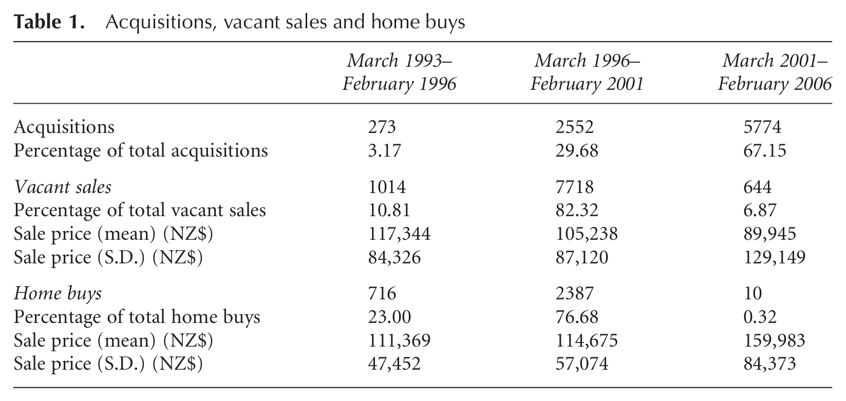
Table 1 summarises the number of acquisitions, vacant sales and Home Buys for the three periods. One stark illustration of the difference in philosophies towards state housing between the National and Labour governments is the almost complete disappearance of Home Buys after 2001 due to the Labour government terminating the Home Buy scheme when elected in late 1999. Table 1 also presents sale price means and standard deviations for vacant sales and Home Buys (similar data are not presented for acquisitions since the latter are a mixture of purpose-built houses and market purchases). Other than in the final period, which saw few sales, the mean sale prices for vacant sales and Home Buys were similar to one another. However, the standard deviation for vacant sales is much larger than for Home Buys reflecting the policy intent to sell vacant state houses in very high-priced areas as well as in areas in which there was little demand for housing such as in rural areas (which tended to coincide with low prices).
Acquisitions, vacant sales and home buys
We obtain 1991, 1996, 2001 and 2006 census data for the number of private dwellings in each census area unit (or CAU) which corresponds to a city suburb or small town (mean population approximately 1500). 2 When examining determinants of state house sales, we alternatively use the stock of state houses and the stock of total private dwellings as denominators. The former is relevant to examining the likelihood that a given state house in an area will be sold, while the latter is relevant to the question of which type of area experienced proportionately higher or lower sale or acquisition flows. Acquisitions are expressed as a ratio of total private dwellings only, since use of the stock of state houses as the denominator would make little sense for areas where there were few or no state houses initially.
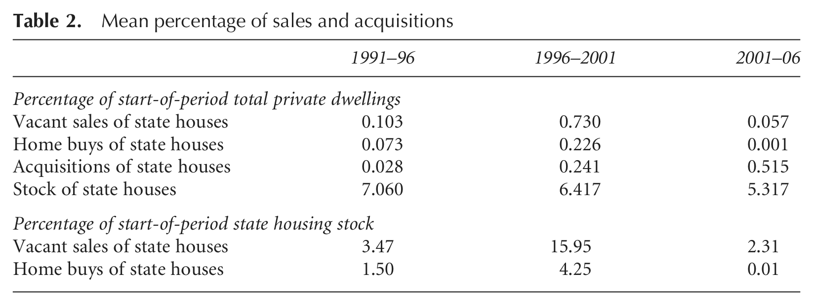
The HNZC dataset has information for 1136 CAUs, whereas the census data contain information for all 1859 CAUs. The remaining CAUs have no state houses throughout the period. Table 2 summarises the mean state housing characteristics over the three census periods, showing a large increase in both vacant sales and Home Buys between 1996 and 2001 and a large decrease in each sales category between 2001 and 2006. These two periods pick up the National and then the Labour government’s respective state housing policies. The mean percentages of sales relative to total private dwellings appear small. However, as a proportion of the initial state housing stock, the sales proportions are material: over 1996–2001, almost 16 per cent of initial state houses were sold as vacant sales and a further 4 per cent as Home Buys.
Mean percentage of sales and acquisitions
We use census data on incomes and demographic characteristics pertaining to the usually resident non-institutionalised adult population for each area (Stillman and Maré, 2008). These variables allow us to control for the population characteristics of areas in our analysis. Rather than include a large number of separate, highly collinear characteristics for each area in the analysis, we include the average income of an area together with a summary measure that proxies the degree of socioeconomic hardship of each CAU. We calculate this summary measure using principal component analysis on a large number of census variables. 3 The first principal component (labelled Socioeconomic) is used as a measure of socioeconomic hardship for each area, where a higher value indicates greater socioeconomic hardship. This variable is similar to the widely used New Zealand Deprivation Index (NZDep), as in Salmond and Crampton (2002), with the two variables having a correlation coefficient of 0.82 in 2001. Table 3 (together with its Notes) lists all variables that comprise the Socioeconomic factor, highlighting those variables that have a correlation coefficient of at least 0.2 (in absolute value) with the factor. As well as income and unemployment, the variables that have a high correlation with Socioeconomic are mostly demographic in nature. There are high correlations of Socioeconomic with the ethnic variables (including the percentage of the population that are of indigenous Maori and Pacific Island ethnicity), relationship status and qualifications.
Correlation of socioeconomic hardship factor with key component variables

Notes: Correlations shown where | correlation coefficient | >0.2. Other variables included in socioeconomic hardship factor are: zero income (percentage); female (percentage); Asian (percentage); other ethnicity (percentage); widowed (percentage); percentage of households with people aged >64; average number of persons per household respectively aged: <5; 5–12; 18–24; >64.
We also obtain house sale price data from Quotable Value New Zealand (QVNZ), a state-owned entity that maintains a dataset of all property sales. We use the log of the sale-weighted median real sales price for residential dwellings (in 1991 NZD) for each area in each of the census years. 4
4. Modelling Approach
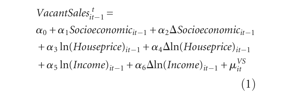
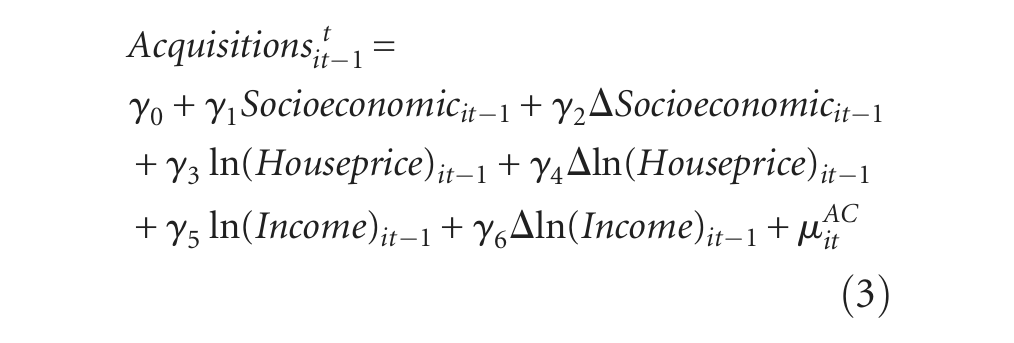
We hypothesise that the probability of sale (vacant sale or Home Buy) of a given state house in CAU i over t−1 to t (where t is measured in five-year units) is a function of conditions in that CAU at or prior to the start of the period. The timing of our variables is chosen to avoid endogeneity concerns in our regressions. In each case, our dependent variable is a flow variable (of sales or acquisitions) from t−1 to t, while the explanatory variables are levels of state variables at the start of period t−1 (i.e. prior to the sales or acquisitions) and changes in the state variables prior to t−1. Since the explanatory variables do not include any variables that coincide with the timing of the sales or acquisitions, we can estimate the equations using ordinary least squares (OLS) rather than techniques such as instrumental variables that would be required if we had simultaneously determined explanatory variables.
We include three variables as determinants of sales of state houses. First, we hypothesise that sales are a function of the socioeconomic factor, Socioeconomic, of CAU i in t−1 (i.e. at the start of the interval) and its prior change (from t−2 to t−1) indicating the degree to which the area was already ‘up-and-coming’. We expect that sales will be higher where socioeconomic hardship is low and/or in areas that were already ‘improving’. As shown in Table 3, the socioeconomic factor comprises a range of demographic variables plus the logarithm of real income, ln(Income). It is possible that incomes have a separate influence on sale probability relative to the demographic components, so we also include the start of period ln(Income) and its prior change as explanatory variables in the sales equations.
We hypothesise that sale probability is affected negatively by the level of local house prices in t−1 (reflecting affordability constraints) and by the prior change in house prices between t−2 and t−1. The prior change in house prices may be a better indicator (than the start-of-period price level) of the perception of whether house prices were expensive for the area since it abstracts from the influence of unchanging amenities such as coastal location or proximity to the city. We have conducted the analysis with respect to house prices in two separate ways, by including the log of the real house price, ln(Houseprice) and the log of the real house price relative to mean income of the area. While the latter specification controls for differing incomes across the country (Lewis and Stillman, 2007), results are very similar and we present only the results using ln(Houseprice).
The resulting equations for the number of vacant sales (

Similarly, the equation for the number of acquisitions (
In each of equations (1)–(3), where the dependent variable is expressed as a ratio of total private dwellings, we add an additional term (StateHouseStock), defined as the ratio of the state house stock to total private dwellings. We do so since, at least for the sales variables, the number of sales that can take place in an area (relative to the total housing stock) is constrained by the initial number (or density) of state houses in the area.
For expositional purposes, we show equations (1)–(3) as having constant coefficients across the two five-year time-periods in our data. Consistent with the differing policy approaches of the two governments across the period, we reject constant coefficients within a panel regression for each variable. Thus, we estimate all equations separately for the two intercensal periods.
While equations (1)–(3) show the hypothesised determinants of sales and acquisitions, our main focus is to ascertain the effects of state house sales and acquisitions on subsequent community outcomes. We model the impacts of these policies on three outcome variables between t and t+1,
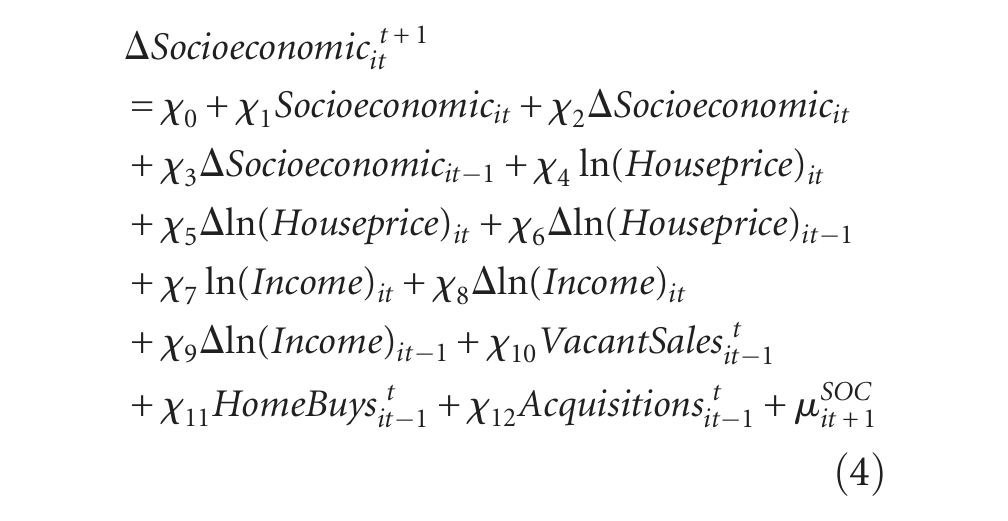
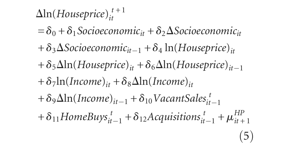
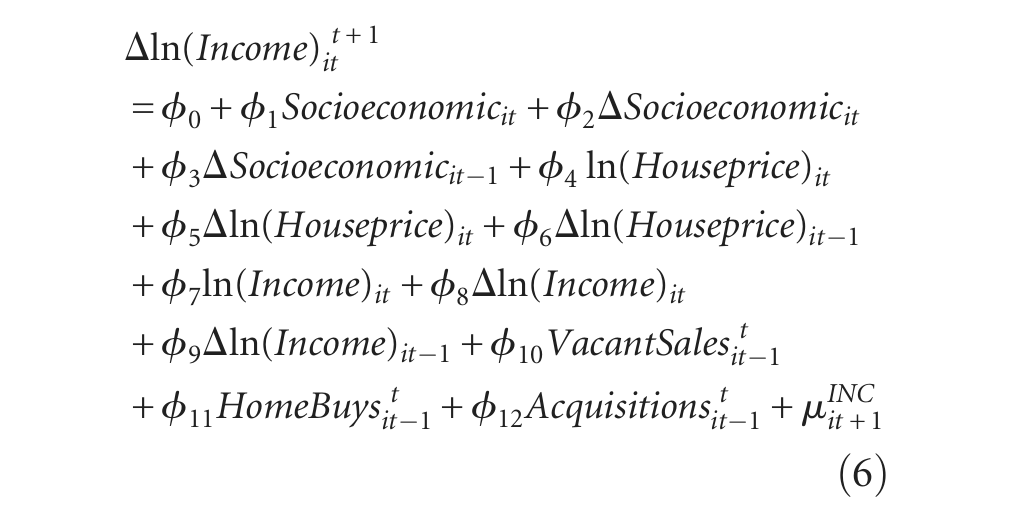
Our key focus in interpreting results from equations (4)–(6) is on the impacts of VacantSales, HomeBuys and Acquisitions on future socioeconomic, income and house price outcomes. Our hypotheses, derived from the literature cited earlier, are that extra Acquisitions will increase socioeconomic hardship in an area and reduce house prices and incomes, extra HomeBuys will increase house prices and reduce socioeconomic hardship (without necessarily affecting incomes), while extra VacantSales will have little effect on any of the outcome variables given that one tenant may be swapped for another.
5. Sale and Acquisition Determinants
Table 1 showed that very few acquisitions occurred over 1991–96 while very few Home Buys and relatively few vacant sales occurred over 2001–06. We therefore present results for the determination of acquisitions over the latter two periods (1996–2006) and for the determination of sales for the former two periods (1991–2001). Equation (3) provides the specification for the determinants of acquisitions, while equations (1) and (2) provide the specifications for vacant sales and Home Buys respectively. Table 4 presents the estimation results for the determinants of Acquisitions, VacantSales and HomeBuys, where the denominator is start-of-period total private dwellings; Table 5 presents corresponding results for the sales variables where state house stock is the denominator. All equations are estimated by weighted OLS (where the weights reflect the population in each CAU), with robust standard errors reported. 5
Acquisition, vacant sale and home buy determinants (percentage of total private dwellings)

Notes: **p<0.01; *p<0.05; +p<0.10, using robust standard errors. All estimates use population-based weights. Socioeconomic is the socioeconomic hardship factor (1st principal component of variables listed in Table 3). The state house stock is expressed as a percentage of total private dwellings.
Vacant sale and home buy determinants (percentage of state housing stock)
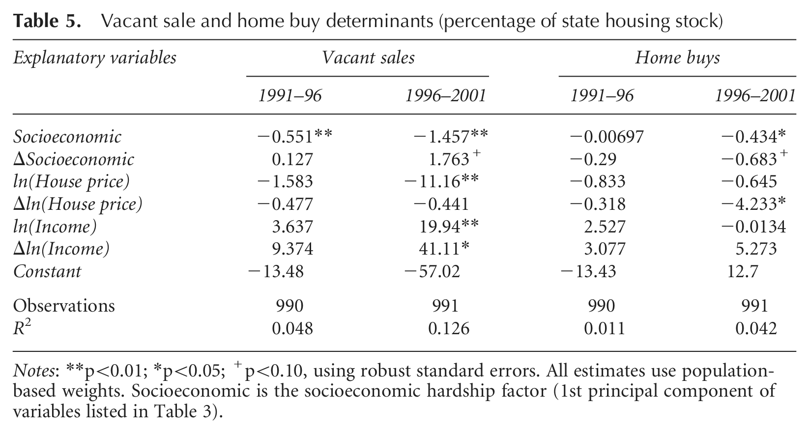
Notes: **p<0.01; *p<0.05; +p<0.10, using robust standard errors. All estimates use population-based weights. Socioeconomic is the socioeconomic hardship factor (1st principal component of variables listed in Table 3).
Acquisitions are higher in areas with greater socioeconomic hardship, consistent with the policies of successive governments to target social housing to areas of greatest need. The results also indicate a positive relationship between initial house prices and acquisitions. This relationship may in part be due to a large number of acquisitions occurring on the outskirts of urban areas where there was available land but where existing houses were relatively expensive (Olssen et al., 2010). Auckland (New Zealand’s largest city) has both a high prevalence of deprived areas and high house prices relative to other parts of New Zealand. Olssen et al. document that a high proportion of acquisitions occurred in Auckland, thus yielding a positive relationship between acquisitions and the level of house prices. The estimates indicate a negative relationship between acquisitions and the prior change in house prices for the 2001–06 period (when 67 per cent of acquisitions occurred). This result indicates that, once the effects of house price levels are controlled for, acquisitions predominantly occurred in areas that had become less expensive relative to previous levels, consistent with state purchasers targeting ‘value for money’ areas when acquiring houses.
Tables 4 and 5 reveal a strong, inverse relationship between the number of vacant sales and the degree of socioeconomic hardship in an area, in accordance with the policy intention of decreasing state housing density in more affluent areas. There is also an inverse relationship between vacant sales and house prices. Thus, after controlling for incomes and other socioeconomic factors, purchasers preferred to purchase a state house in less expensive areas.
In keeping with the vacant sale results, Home Buys also show an inverse relationship with the level of socioeconomic hardship; thus, ceteris paribus, tenants were less likely to purchase their house if they lived in a more socioeconomically deprived area. High house prices and high house prices relative to prices five years earlier (especially over 1996–2001, when 77 per cent of Home Buys took place) acted as a disincentive to purchasers. Incomes do not appear to have had an impact over and above other socioeconomic factors or house prices except over 1996–2001 when we find that Home Buys were more prevalent in areas that had experienced relative decreases in real incomes over the prior five years.
Together, these results indicate that existing state house tenants were more likely to purchase their house if they were in a more desirable area but one that was not highly priced relative to its socioeconomic level. One reason that house prices may have been low in relation to the existing socioeconomic level in these areas is that the prices were reflecting an expectation that the area would continue to experience a decline in incomes and/or other elements of socioeconomic hardship. Thus, ceteris paribus, existing tenants may have been more able to afford to buy in an area that was expected to deteriorate rather than in an up-and-coming suburb.
6. The Impact of State House Sales and Acquisitions
A key difficulty encountered in previous studies that have investigated the impact of homeownership on societal outcomes has been the inability to isolate an exogenous event that causes a switch in tenure status from tenant to homeowner (or vice versa). The state house sales programme in New Zealand, driven by political philosophy, is one such exogenous event. This is particularly the case in the way that the National government’s Home Buy scheme enabled existing state house tenants to purchase their existing residence, an option which had previously been denied to tenants. We investigate whether an increase in acquisitions, vacant sales and, in particular, Home Buys led to subsequent changes in socioeconomic hardship, incomes and house prices in an area. The house price outcomes specifically provide a market-based summary measure of changes in community wellbeing or perceived amenity values for a local area.
We concentrate on the impacts of sales and acquisitions conducted over the 1996–2001 period since the bulk of sales occurred over this period and this period also saw sizeable acquisition activity. Equations (4)–(6) provide the specifications that we estimate, with the columns in Table 6 presenting the results for the changes to the three outcome variables (i.e. ΔSocioeconomic, Δln(HousePrice) and Δln(Income)).
Impacts of prior vacant sales, home buys and acquisitions on outcomes
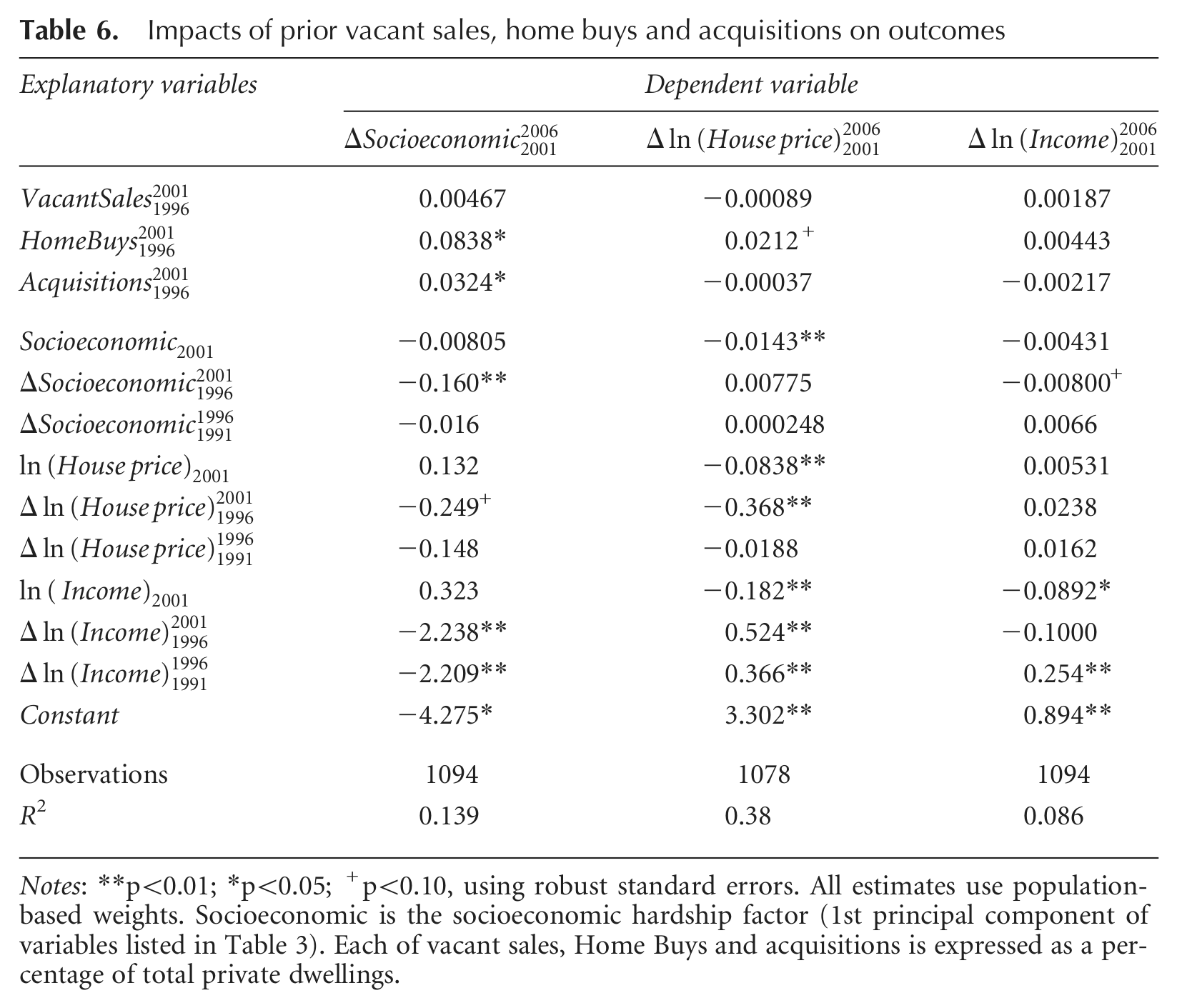
Notes: **p<0.01; *p<0.05; +p<0.10, using robust standard errors. All estimates use population-based weights. Socioeconomic is the socioeconomic hardship factor (1st principal component of variables listed in Table 3). Each of vacant sales, Home Buys and acquisitions is expressed as a percentage of total private dwellings.
Prior to examining the impacts of the variables of policy interest (VacantSales, HomeBuys and Acquisitions), we note some other key features of the estimated equations. As is commonly the case with cross-sectional regressions, explanatory power of the three equations is only moderate (the highest R2 is 0.38) but nevertheless several strongly significant results are apparent. An increase in socioeconomic hardship (column 1) is associated significantly with prior decreases in house prices and incomes; thus decreases in the latter variables help to predict subsequent increases in socioeconomic hardship. Changes in house prices (column 2) are positively associated with prior changes in incomes over each of the two previous intercensal periods. Furthermore, current changes in incomes (column 3) are positively associated with prior changes in incomes. Together, the house price and income results indicate marked persistence in the dynamics of incomes and house prices across areas. In turn, an area’s income and house price dynamics help to predict subsequent changes in the area’s degree of socioeconomic hardship.
Turning to the three policy variables of interest, column 1 of Table 6 indicates a positive relationship between the change in socioeconomic hardship over 2001–06 and the level of acquisitions over 1996–2001. This result is entirely in keeping with the purposes of the acquisition programme which was to house those parts of the socioeconomic spectrum most in need of housing and broader social assistance. An increase in state house acquisitions will therefore directly increase the number of people suffering from socioeconomic hardship within the relevant area.
Socioeconomic changes have no significant relationship with prior vacant sales while, contrary to our hypothesis, an increase in Home Buys is associated with a subsequent increase in our measure of socioeconomic hardship for an area. Increased Home Buys (or vacant sales or acquisitions) have no effect on subsequent real incomes (column 3), so the latter cannot be the cause of the increase in an area’s degree of socioeconomic hardship that followed increased Home Buys.
We investigate in more depth the reasons for the increase in an area’s socioeconomic hardship factor following an increase in Home Buys by regressing each element that comprises the socioeconomic hardship factor on the same variables included in equation (5). Table 7 lists all equations for which Home Buys has a significant impact on any individual element within Socioeconomic. (It also includes the Home Buys equation from Table 6 for comparison; for conciseness, the table does not list the coefficients on the control variables which are still included as before.) The results show that Home Buys precede a range of demographic changes, all but one of which (Divorced/Separated) is consistent with an increase in the socioeconomic hardship factor. Greater Home Buys are seen to precede increases in the proportion of disadvantaged minorities in the area, people with fewer qualifications, a younger age structure and fewer married and/or couple households. These results are consistent with the results from equation (2) on the determinants of Home Buys whereby Home Buys over 1996–2001 were, ceteris paribus, greatest in areas with low and declining house prices. One possible reason that existing tenants could afford to purchase their house in particular areas was that those areas were on a path to lower socioeconomic outcomes and this was reflected in recent changes in house prices.
Impacts of vacant sales, home buys and acquisitions on socioeconomic components

Notes: **p<0.01; *p<0.05; +p<0.10, using robust standard errors. All estimates use population-based weights. Equations presented are those for which HomeBuys is significant for individual components of Socioeconomic. The first equation in Table 7 reproduces the equation from Table 6 for comparison. Socioeconomic is the socioeconomic hardship factor (1st principal component of variables listed in Table 3). All equations include all control variables listed in Table 6 (not reported here), and have 1094 observations. Each of vacant sales, Home Buys and acquisitions is expressed as a percentage of total private dwellings.
Returning to Table 6, the results indicate that, after controlling for prior socioeconomic, income and house price levels and trends, there is a positive relationship between the percentage of Home Buys and the subsequent change in house prices in an area (column 2). The estimate suggests that a 1 percentage point increase in Home Buys as a proportion of total private dwellings in an area is associated with a subsequent 2 per cent increase in real house prices in that area over and above other local house price influences. 6 This result occurs in spite of findings, from Table 7, that Home Buys were most prevalent in areas in which a range of socioeconomic elements were deteriorating. These deteriorating trends may otherwise have been expected to reduce house price growth. The house price results accord with the hypothesis that a change in the housing tenure status of a given resident from state tenant to homeowner (as occurred, by definition, with the Home Buy scheme) has positive spin-offs for the local community—even where that community may have been on a path towards a lower socioeconomic status. The positive externalities from the change in tenure status from tenant to homeowner are capitalised into a higher price of houses in the local area after controlling for other prior influences.
Neither vacant sales nor acquisitions had any effect on subsequent house price changes. The acquisitions result is perhaps surprising given that acquisitions increased the measured socioeconomic hardship of an area, consistent with the policy intent. The practice of ‘pepper-potting’ acquired state houses amongst a broader community, adopted over this period (mitigating intense concentrations of state housing), may be one reason that local house prices were unaffected by acquisition patterns (Schrader, 2005).
Vacant sales differ from Home Buys in that, by definition, a vacant sale corresponds to a change in resident whereas the resident remains the same with a Home Buy. Some vacant sales resulted in a shift in tenancy status for the house from having a tenant to having a homeowner, but others resulted in sale of the house to a landlord, thereby replacing one tenant with another. Compared with the Home Buy scheme, there is therefore less reason to expect that vacant sales led to changed outcomes for a community, consistent with our results.
7. Conclusions
New Zealand’s state housing policies over the two decades following 1990 gave rise to two natural experiments regarding the sale and acquisition of state houses. The 1990s National government sought to reduce the overall state house stock and to redirect it towards areas most in need, while the post-1999 Labour government sought to increase the overall stock, often through acquiring new state houses in fringe urban areas. We utilise these natural experiments to examine both the determinants of state house sales and acquisitions, and the impacts that these flows had on subsequent changes in local socioeconomic hardship, incomes and house prices.
Acquisitions tended to occur in areas with high socioeconomic hardship, in accordance with policy intentions. By contrast, vacant sales tended to occur in areas of lower socioeconomic deprivation and in lower-priced areas (after controlling for socioeconomic factors). We also find that a greater number of Home Buys occurred in areas that had lower existing socioeconomic hardship and in areas with low or falling relative house prices. These findings are in accordance with our hypotheses. Over 1996–2001, Home Buys also tended to occur in areas with falling real incomes. The ability of an existing tenant to purchase their state house may have reflected a situation in which house prices reflected an expectation of continued negative trends for the area which made houses more affordable in those areas.
Having determined which factors must be controlled for in determining the prevalence of each of acquisitions, vacant sales and Home Buys, we analysed the impacts of sales and acquisitions (over 1996–2001) on subsequent changes in local socioeconomic hardship, incomes and house prices (over 2001–06). Vacant sales had no impact on subsequent outcomes for any of these three variables. Areas that experienced a relatively high level of acquisitions witnessed a subsequent increase in socioeconomic hardship, consistent with policy intentions. Areas that experienced a relatively high percentage of Home Buys witnessed a subsequent deterioration in certain elements of their socioeconomic structure but at the same time they experienced a subsequent increase in real house prices. Closer examination of these impacts indicates that areas that had high Home Buy proportions experienced subsequent increases in the demographic groups most strongly represented in areas with greatest socioeconomic hardship. This is consistent with the finding that Home Buys were strongest in areas with low and/or declining house prices, reflecting a forward-looking expectation that certain socioeconomic (particularly demographic) elements of the area were likely to lead to greater local hardship. Despite these demographic trends, the increase in real house prices in these neighbourhoods that followed greater Home Buy activity is indicative that the change in tenure status from tenant to homeowner was reflected in superior neighbourhood outcomes that was internalised into subsequent house price growth for the area.
Future work could use unit record data to analyse whether neighbouring properties benefit more from Home Buy sales than do more distant properties. If so, this would suggest that observable characteristics of the house (such as house maintenance) or of the household (such as residents’ behaviour) may have changed as a result of the purchase decision. If the effect is spatially more diffuse, the neighbourhood benefits may reflect increased social capital whereby the purchaser participates more fully in local community activities such as crime-reduction schemes. New Zealand’s natural experiments with state housing, driven by the differing political philosophies of alternating governments, therefore offer valuable opportunities to investigate the impacts that tenure status can have on individual and community outcomes. Our results suggest that the Home Buy scheme, which offered tenants a hitherto unavailable option to become the owner of their existing residence, did affect community outcomes positively, but the exact source of those benefits is still to be determined.
Footnotes
Acknowledgements
The authors thank Housing New Zealand Corporation for confidential access to state housing data, and also thank the editor and two anonymous referees for their comments on a prior version of this paper.
Funding
The authors would like to thank the Royal Society of New Zealand Marsden Fund (07-MEP-003) and the Motu Foundation for funding assistance.