Empowerment for whom? The impact of community renewal tax incentives on jobs and businesses

How RC/EZ/ECs work

For half a century, the USA has experimented with place-based urban revitalisation initiatives including (1) urban renewal in the 1950s (Halpern, 1995); (2) Model Cities in the 1960s (O’Connor, 1999); (3) Urban Development Action Grants in the 1970s (Rich, 1989); (4) state enterprise zones in the late 1980s (Boarnet, 2001; Lavin and Whysall, 2004); and (5) Comprehensive Community Initiatives in the late 1990s (Kubisch, 2010). In 1994, the federal government returned to an interest in place when US HUD designated eight Empowerment Zones and 65 Enterprise Communities in order to build capacity and increase economic opportunity in high-poverty neighbourhoods (Lavin and Whysall, 2004). See Figure 1 for a summary of benefits, which included social services grants, loan guarantees and tax incentives for businesses (US HUD, 2012). In particular, the EZ wage credit allowed a business to take 20% of qualified wages up to US$3000 off their taxes for each employee they hired who lived and worked in the designated area. This emphasis on place and people was an attempt to encourage businesses to hire from the EZ. In 1997, US HUD designated 15 Round II EZs and in 2001, US HUD designated 8 Round III EZs and 40 RCs (US HUD, 2012). The RC wage credit was 15% of qualified wages, capped at US$1500 per employee. Congress also extended the Round I EZs to match the expiration date of Round III.

OPEN IN VIEWER

Figure 1.

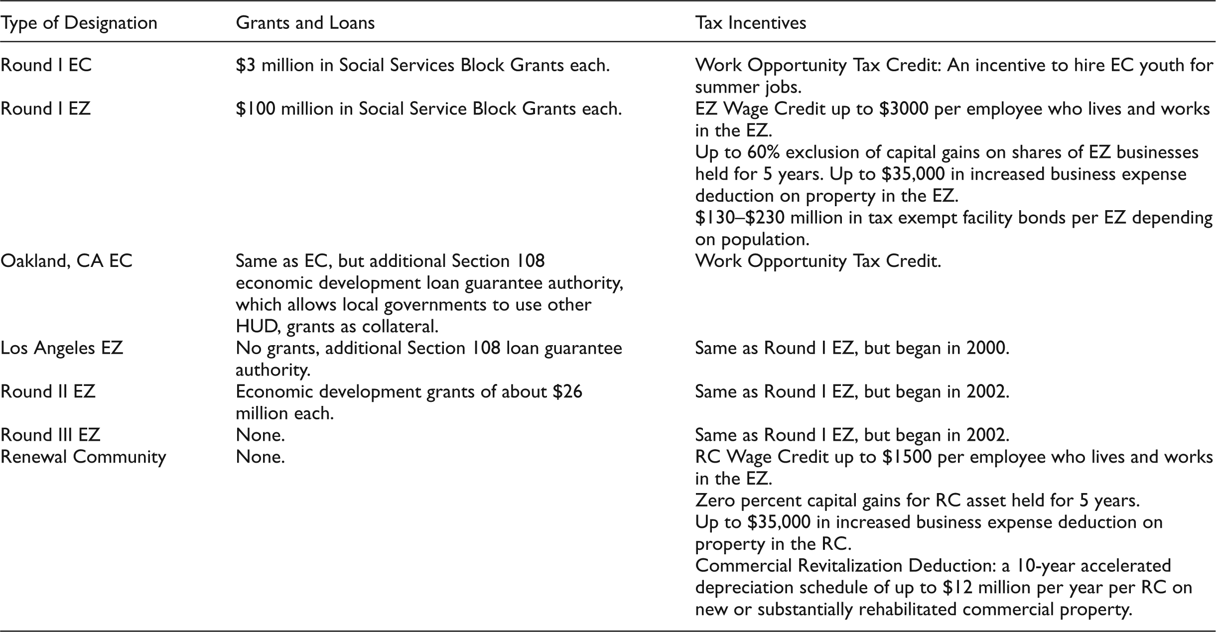
Summary of urban RC/EZ/EC benefits.

Local governments partnered with community organisations to administer or promote benefits. For example, many EZs partnered with a Small Business Administration One-Stop Capital Shop to link entrepreneurs in the EZ to business assistance services (US HUD, 2005). RCs and EZs also worked with minority and immigrant businesses (US HUD, 2008). A US Government Accountability Office (US GAO) (2004) report noted an increasing utilisation of tax incentives between 1995 and 2001. By 2008, businesses claimed US$3.2 billion in RC and EZ wage credits, benefited from US$643 million in tax-exempt bonds, and were able to accelerate the depreciation of US$1.7 billion of new commercial real estate (US GAO, 2010). Hanson (2009) estimated that employers took wage credits for 24.2% of employees in the EZ.

The organisation and implementation of these programmes were complex (US GAO, 2004). To apply, local governments prepared strategic plans with substantial participation from neighbourhood residents and other stakeholders. The first eligibility criterion was that RC/EZ/EC areas had to be selected from 1990 census tracts with at least 20% poverty and high unemployment, with some exceptions. In the RC programme, unemployment needed to be at least 9%. For Round II and III EZs, Congress relaxed the eligibility criteria, such that designed areas were not exclusively from the poorest census tracts (Greenbaum and Bondonio, 2004). After the EZ/EC applicant met objective eligibility thresholds, US HUD reviewers subjectively scored each strategic plan. In contrast, RC selection was objective and based solely on ranking applicants’ poverty and unemployment with a bonus point for having been an EZ/EC.

Although the RCs expired in 2009, Congress extended the EZs to 2013. The White House (2011) asked Congress to replace EZs with 20 new Growth Zones (GZs). The GZ would last four years in one contiguous area each but otherwise be similar to the EZ (US Department of the Treasury, 2011). The GZ benefits include an accelerated depreciation schedule to allow businesses to deduct 100% of the adjusted basis in the first year of service. The GZ wage credit would reimburse 20% of the first US$15,000 of wages paid for work performed inside the GZ by residents of the GZ and 10% of wages for residents who work elsewhere. In 2013, President Obama renamed the proposal Promise Zones (PZ) (White House Office of the Press Secretary, 2013). Does the literature support place-based initiatives?

Review of empirical research on EZs

Both equity and efficiency concerns are raised in the literature about place-based policies. The subsidies could become capitalised in land rents and pass on the costs to inner-city residents, who would have been better served with investments in schools, income transfers or enforcement of anti-discrimination policies (e.g. Lavin and Whysall, 2004; Levine, 1999; Quigley, 1994). However, others reject this zero-sum game argument and point out that a region could be better off if resources were expended to create jobs in a high unemployment area (Bartik, 1991). Finally, Marcuse (1997) argues that EZs would be a better fit for immigrant enclaves than for high-poverty African-American neighbourhoods because immigrants have more place-based social capital to leverage for entrepreneurship.

Evaluations have estimated the impact of state and federal EZ programmes on warehouse inventory, real estate capitalisation, wages, vacancy, poverty and unemployment. Identification of a causal policy impact for these programmes has been confounded because the selection of winners was done based on need and not randomised. In the 1980s and early 1990s, SEZ evaluations were subject to criticism of omitted control variables, geographic imprecision, selection bias and non-generalisability (Boarnet, 2001; Ladd 1994; Wilder and Rubin 1996). The SEZ studies used different designs to address selection bias that in turn were applied to Federal EZ/ECs (FEZ) that include (1) panel data methods and instrumental variables (Angrist and Pischke, 2008), (2) regression discontinuity (RD) (Thistlethwaite and Campbell, 1960) or (3) propensity score matching (Rosenbaum and Rubin, 1983). In general, the FEZ is compared before and after the intervention with comparison to tracts that are (1) within the same city; (2) within a certain distance; or (3) in other cities with similar characteristics. Findings vary by outcome, sample, counterfactuals and estimation method. To date, only Round I FEZs have been evaluated. See Figure 2 for a summary of key FEZ studies.

OPEN IN VIEWER

Figure 2.

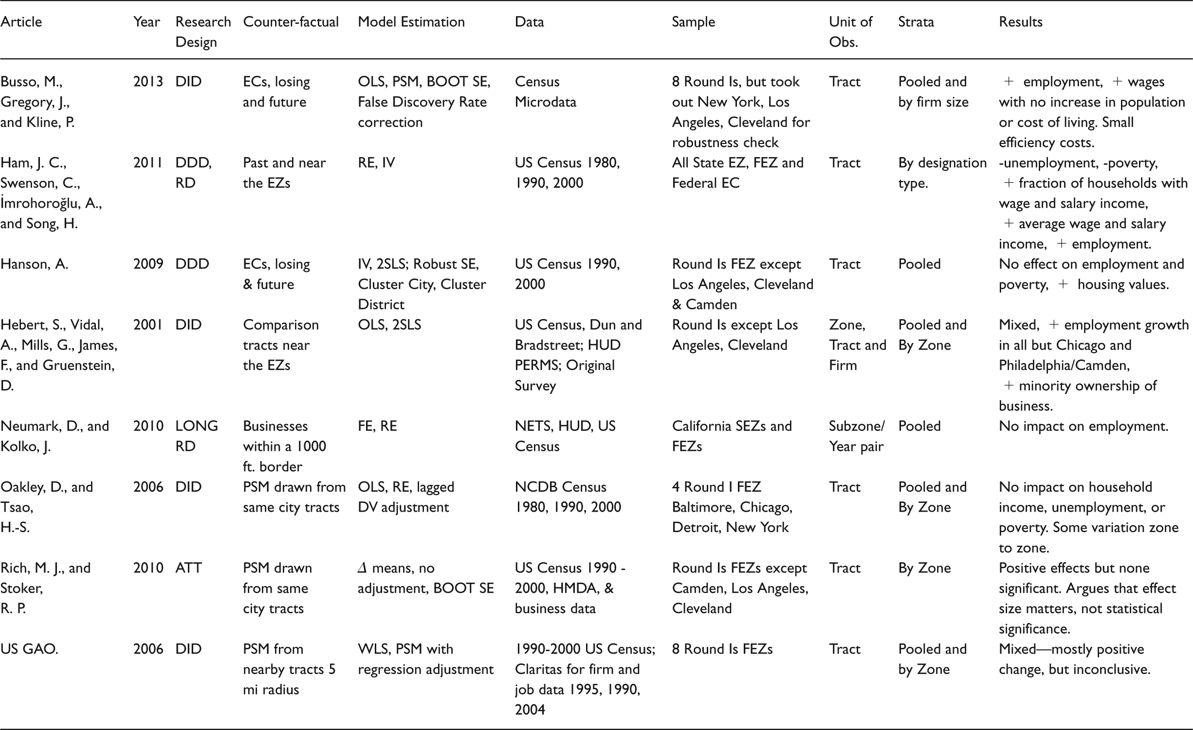
Summary of key empirical articles.

Some studies were sceptical. Oakley and Tsao (2006) used the Neighborhood Change Data Base (Tatian and Kingsley, 2003) to conclude that there was no impact on logged average household income, unemployment and poverty in four Round I EZs. They did find improvements in some outcomes in some zones. The US GAO (2006) found improvements in the number of businesses in FEZs in Camden, Cleveland and New York. They also found increased job growth in Baltimore, Camden, Detroit, Upper Manhattan and Philadelphia, but decreased numbers of jobs in Atlanta, the Bronx, Chicago, Cleveland, Los Angeles and Philadelphia. US GAO (2006) was not confident in attributing a causal relationship because their control areas did not have covariate balance, common support, or a reasonable qualitative justification based on their conversations with zone administrators. For the California SEZ and FEZ, Neumark and Kolko (2010) found no impact on jobs whether or not those areas that also had been designated FEZs using data from the National Establishment Time Series Database (NETS) (Walls, 2008). For the Federal EZ programme, Hanson (2011) used political and economic instrumental variables (IV) to control for selection bias and found no difference in employment outcomes but did find an increase in property values, suggesting that the programme did make the neighbourhood more expensive without benefiting workers.

Other evaluations have found a preponderance of evidence for impact. For example, Hebert et al. (2001) used data from Dun and Bradstreet and found increased job growth in four of the six FEZs and an increase in the number of minority-owned businesses compared with a group of adjacent high-poverty tracts in the same city. Rich and Stoker (2010) agreed that the programme was impactful, and argued that most of the FEZs had positive outcomes for poverty, unemployment, housing starts and business. They noted that having large effect sizes was more important than statistical significance because of the small sample size and policy-makers’ need for practical results. Ham et al. (2011) argued that previous studies did not adequately distinguish between local government policy and location advantage, so they combined RD with a random growth curve model to account for baseline conditions and found a positive effect on employment. An RD design exploits the treatment assignment mechanism, in this case the geographic border of the EZ, to identify a local average treatment effect by comparing observations inside the border to those outside the border. Finally, Busso et al. (2013) used census microdata to identify comparison areas from eligible losing applicants for an FEZ designation in other jurisdictions and found an overall increase in employment and reduced poverty for Round I EZs. Others rejected within-city comparisons and RD because of spillover effects and argued that application selection bias was more important to overcome than unobserved policy variation (Busso et al., 2013; Hanson and Rohlin, 2012).

In short, while programme expenditures have been large, the results of these programmes on employment and business outcomes have been mixed. Therefore the basic question of impact on jobs and businesses is open as the programme evolves. While previous studies have focused primarily on Round I FEZs, this study adds to the literature by being the first to analyse the impact of Round II EZs, Round III EZs and RCs. While propensity score matching has been commonplace, covariate balance has been a problem. To move the literature forward, I use a state-of-the-art propensity score-matching algorithm called genetic matching (GenMatch). For a counterfactual, I am comparing designated tracts to similar distressed tracts within the same state. In order to get better geographic and temporal precision, like Neumark and Kolko (2010), I use the NETS, which contains address-level, annual business data over a 18-year period. To estimate policy impacts, I use adjusted interrupted time series analysis, which is appropriate for cross-sectional time series data. Specifically, this paper tests three hypotheses:

Hypothesis One: The RC/EZ/EC areas have a one-time-increase in jobs and an increased growth rate in the post-intervention period compared with the pre-intervention period and the control area (JOBS).

Hypothesis Two: The RC/EZ/EC areas have a one-time increase in the number of new establishments and increased establishment opening rate in the post-intervention period compared with the pre-intervention period and the control area (OPENINGS).

Hypothesis Three: The RC/EZ/EC areas have a one-time decrease in the number of closed establishments and decreased establishment closure rate compared with the pre-intervention period and the control area. (CLOSURES).

I present results in pooled form, by zone and stratified by the subpopulations of all tax-incentive eligible establishments, retail establishments (including hotels), establishments with five employees or fewer and minority businesses that are more typical of high-poverty areas.

Data and methods

Data sources and study sample

Outcome data were from the national establishment time series data base (NETS), which has address-level data on establishments in the US from 1990 to 2007 (Walls, 2008). The NETS assembles January snapshots of Dun and Bradstreet data to hold seasonal variation constant. To provide some geographic and demographic variation to test Marcuse’s (1997) intuition about the relative fit of the EZ concept to immigrant versus African-American neighbourhoods, I selected California because it is a Pacific state with high immigration and my institution had a NETS license. California’s industry includes agriculture, entertainment, technology and tourism. I purchased Tennessee data because it had the lowest proportion of foreign-born among the RC/EZs and included African-American neighbourhoods. Tennessee is in the Southeast and known for agriculture, bourbon, industry and music-related tourism.

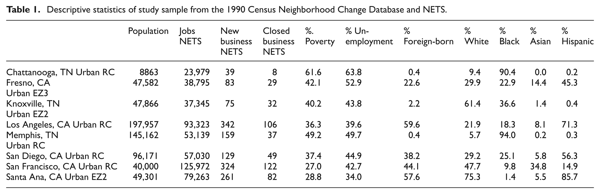
Since 1995, US HUD has designated 117 RC/EZ/ECs. The sample has the following FEZs and RC: (1) Chattanooga, TN RC (n = 5), containing some industrial areas mixed with mostly African-American neighbourhoods surrounding the downtown riverfront; (2) Knoxville, TN Round II EZ (n = 23), adjacent to the University of Tennessee, a flagship research university, containing portions of the downtown riverfront and industrial reuse sites; (3) Memphis, TN RC (n = 18), containing the fabled Beale Street, home of the Blues, as well as an international airport home to the headquarters of FedEx, an air delivery company; (4) Fresno, CA Round III (n = 16), an industrial and warehousing city in California’s agricultural region; (5) Los Angeles, CA RC (n = 39), containing Central American, Chinese, Korean and Filipino ethnic enclaves between downtown, the University of Southern California, and Hollywood; (6) San Diego, CA RC (n = 18), a region extending from the airport west through downtown to African-American and Latino neighbourhoods; (7) San Francisco, CA RC (n = 9), wrapping along Market Street from the Financial District, past Union Square, the theatre district and the Tenderloin to a Latino enclave called the Mission; and (8) Santa Ana, CA Round II (n = 17), containing portions of downtown, the Santa Ana Zoo, and an industrial park in a Latino neighbourhood. Each treatment tract (N = 145) is matched to a set of weighted control tracts within the same state. See Table 1 for descriptive statistics. Note that some ‘distressed areas’ have four jobs per resident because they include major commercial or industrial areas.

OPEN IN VIEWER

Table 1.

Descriptive statistics of study sample from the 1990 Census Neighborhood Change Database and NETS.

	Population	Jobs NETS	New business NETS	Closed business NETS	%. Poverty	% Un-employment	% Foreign-born	% White	% Black	% Asian	% Hispanic
Chattanooga, TN Urban RC	8863	23,979	39	8	61.6	63.8	0.4	9.4	90.4	0.0	0.2
Fresno, CA Urban EZ3	47,582	38,795	83	29	42.1	52.9	22.6	29.9	22.9	14.4	45.3
Knoxville, TN Urban EZ2	47,866	37,345	75	32	40.2	43.8	2.2	61.4	36.6	1.4	0.4
Los Angeles, CA Urban RC	197,957	93,323	342	106	36.3	39.6	59.6	21.9	18.3	8.1	71.3
Memphis, TN Urban RC	145,162	53,139	159	37	49.2	49.7	0.4	5.7	94.0	0.2	0.3
San Diego, CA Urban RC	96,171	57,030	129	49	37.4	44.9	38.2	29.2	25.1	5.8	56.3
San Francisco, CA Urban RC	40,000	125,972	324	122	27.0	42.7	44.1	47.7	9.8	34.8	14.9
Santa Ana, CA Urban EZ2	49,301	79,263	261	82	28.8	34.0	57.6	75.3	1.4	5.5	85.7

Data analysis methods

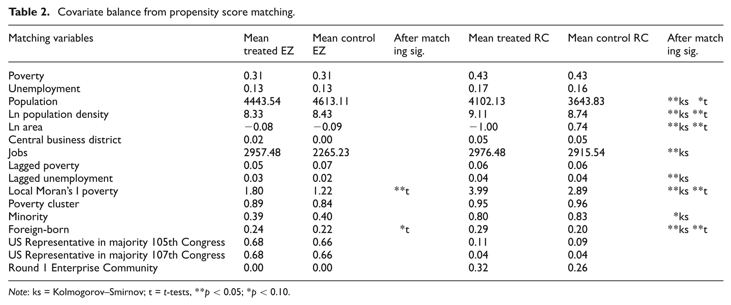
As with previous work (Busso et al., 2013; Oakley and Tsao, 2006; Rich and Stoker, 2010; US GAO, 2006), this study used propensity score matching to make claims about impact. Matching allows estimation of the average treatment effect on the treated (ATT) when two assumptions are met: (1) selection on observables, meaning that the treatment and control groups have no statistically significant differences on any variables that could have influenced selection; and (2) common support (Sekhon, 2009), or as Rosenbaum and Rubin (1983) say, strong ignorability, which means that the treatment and control groups have overlapping distributions on each covariate. I considered covariates balanced if p > 0.10 on all key variables using t-tests and Kolmogorov–Smirnov (KS) tests. I assessed common support using kernel density plots. The RC selection criteria were objective so satisfying the selection on observables assumption was trivial. However, the US HUD selected EZ applications subjectively based on the quality of their strategic plan. In order to accept the results, one has to accept that the quality of the local government’s strategic planning is some function of the matching variables.

Because the RCs had different selection criteria than Round II and Round III EZs (US GAO, 2004), I estimated separate propensity scores for each using the matching variables from the previous section in a multinomial logit model. GenMatch software improves propensity score matching by using non-parametric, iterative processes to better obtain covariate balance between treatment and controls (Sekhon, 2009). I selected one-to-many matching with replacement in order to obtain correct inference and weighted the controls proportionately to improve the estimate of ATT. In general, the estimate of ATT after propensity score matching is estimated by a difference in means. However, this may only be used in a pre-post design (Hartman, 2009). Because the NETS data in this study contained 18 panels, I combined matching with the adjusted interrupted time series (AITS) model from Galster et al. (2004) to identify the impact of an intervention by controlling for past levels and trends:

l i n k ( D V t ) = c + d 1 ( D I M P w c t ) + d 2 ( D I M P g r a n t t ) + e 1 ( D P O S T I M P w c t ) + e 2 ( D P O S T I M P g r a n t t ) + f ( T R I M P t ) + g 1 ( T R P O S T I M P w c t ) + g 2 ( T R P O S T I M P g r a n t t )

(1)

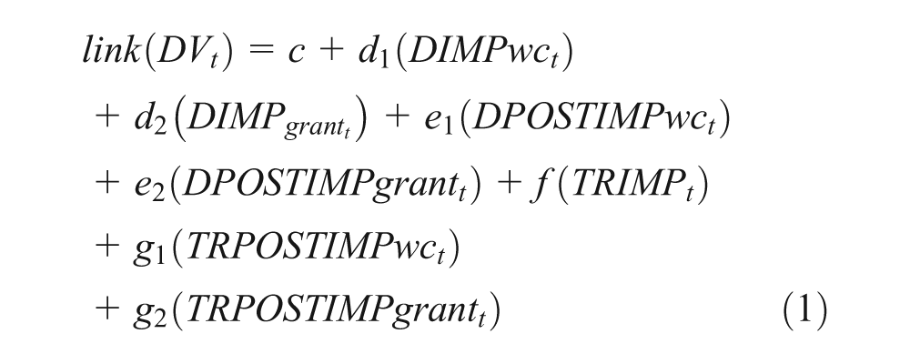
The three dependent variables, DV_t , were the number of jobs, new establishments or establishment closures as reported to Dun and Bradstreet among businesses located in a given census tract. The independent variables were dummy variables for the treatment period, area and trend. First, DIMP_grant identified a census tract in an EZ that received a grant (Knoxville, TN and Santa Ana, CA), where DIMP_wc identified all EZs or RCs because they all received a wage credit, only at different times. Similarly, DPOSTIMP_grant and DPOSTIMP_wc were dummies for an EZ or RC post-impact date, and TRIMP_t was a vector of cardinal numbers, starting at one for the first time period (1990 = 1) and increasing by one for each subsequent time period (2007 = 18 for jobs; 2006 = 17 for establishment openings and closings). Likewise, TRPOSTIMP_grant and TRPOSTIMP_wc were a similar vector of cardinal numbers, starting at the year the grant or wage credits went into effect. TRALL_t numbered the trend in the dependent variable for tracts both inside and outside the EZ or RC while TRPOSTALL_t numbered the trend in all tracts (only post-award) of wage credits or grants, respectively. With regard to interpretation, the key variables of interest were e, the one-time change in the level of the dependent variable and g, the change in the trend over time of the dependent variable. I estimated the model in Stata using negative binomial regression (Hilbe, 2011; Hubbard et al., 2010). ⁵ The coefficients were incident rate ratios, defined as the events per area/time in time 1 over the events per area/time in time 2.

Results

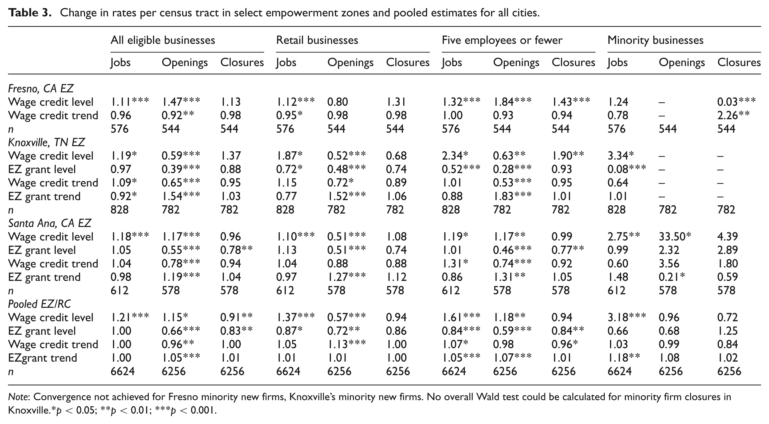
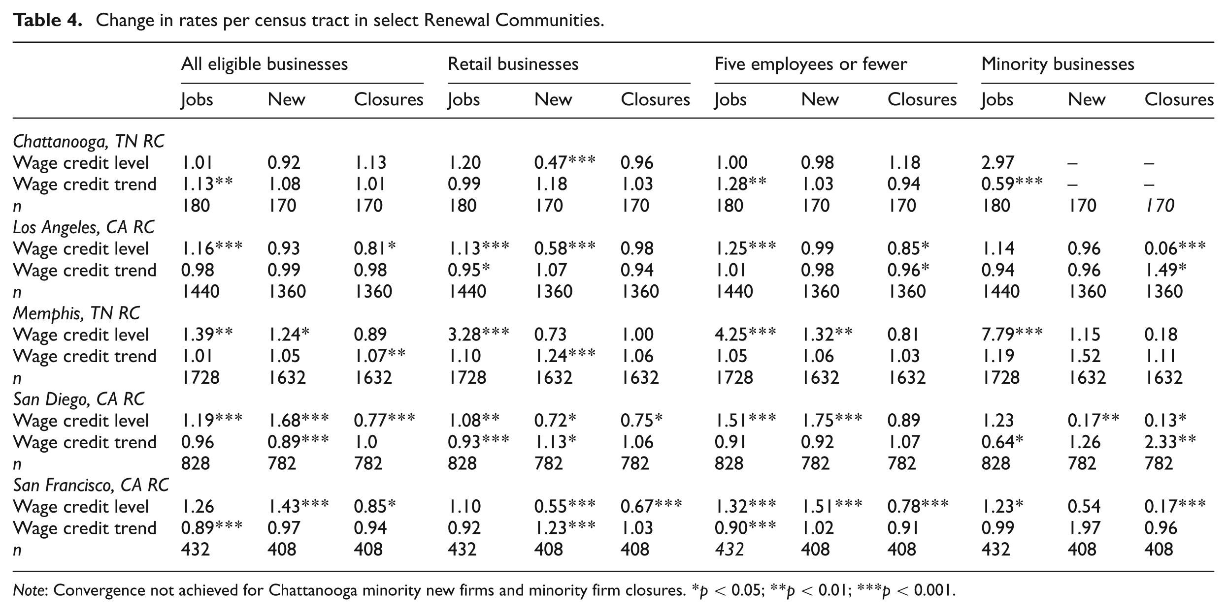
See Table 2 for propensity score balance statistics. Although the RC control groups are not as well balanced as the EZs, the AITS provides a conservative estimate of impact by adjusting for past level and trends in the dependent variables. Since each local government customises implementation of the RC or EZ, it is appropriate to analyse each separately. See Table 3 for a summary of the wage credits and EZ grants impact on jobs, new establishments and establishment closures for FEZs and pooled impacts for all cities in the sample. See Table 4 for the RCs in the sample.

OPEN IN VIEWER

Table 2.

Covariate balance from propensity score matching.

Matching variables	Mean treated EZ	Mean control EZ	After match ing sig.	Mean treated RC	Mean control RC	After match ing sig.
Poverty	0.31	0.31		0.43	0.43
Unemployment	0.13	0.13		0.17	0.16
Population	4443.54	4613.11		4102.13	3643.83	**ks *t
Ln population density	8.33	8.43		9.11	8.74	**ks **t
Ln area	−0.08	−0.09		−1.00	0.74	**ks **t
Central business district	0.02	0.00		0.05	0.05
Jobs	2957.48	2265.23		2976.48	2915.54	**ks
Lagged poverty	0.05	0.07		0.06	0.06
Lagged unemployment	0.03	0.02		0.04	0.04	**ks
Local Moran’s I poverty	1.80	1.22	**t	3.99	2.89	**ks **t
Poverty cluster	0.89	0.84		0.95	0.96
Minority	0.39	0.40		0.80	0.83	*ks
Foreign-born	0.24	0.22	*t	0.29	0.20	**ks **t
US Representative in majority 105th Congress	0.68	0.66		0.11	0.09
US Representative in majority 107th Congress	0.68	0.66		0.04	0.04
Round 1 Enterprise Community	0.00	0.00		0.32	0.26

Note: ks = Kolmogorov–Smirnov; t = t-tests, **p < 0.05; *p < 0.10.

OPEN IN VIEWER

Table 3.

Change in rates per census tract in select empowerment zones and pooled estimates for all cities.

	All eligible businesses			Retail businesses			Five employees or fewer			Minority businesses
	Jobs	Openings	Closures	Jobs	Openings	Closures	Jobs	Openings	Closures	Jobs	Openings	Closures
Fresno, CA EZ
Wage credit level	1.11***	1.47***	1.13	1.12***	0.80	1.31	1.32***	1.84***	1.43***	1.24	–	0.03***
Wage credit trend	0.96	0.92**	0.98	0.95*	0.98	0.98	1.00	0.93	0.94	0.78	–	2.26**
n	576	544	544	576	544	544	576	544	544	576	544	544
Knoxville, TN EZ
Wage credit level	1.19*	0.59***	1.37	1.87*	0.52***	0.68	2.34*	0.63**	1.90**	3.34*	–	–
EZ grant level	0.97	0.39***	0.88	0.72*	0.48***	0.74	0.52***	0.28***	0.93	0.08***	–	–
Wage credit trend	1.09*	0.65***	0.95	1.15	0.72*	0.89	1.01	0.53***	0.95	0.64	–	–
EZ grant trend	0.92*	1.54***	1.03	0.77	1.52***	1.06	0.88	1.83***	1.01	1.01	–	–
n	828	782	782	828	782	782	828	782	782	828	782	782
Santa Ana, CA EZ
Wage credit level	1.18***	1.17***	0.96	1.10***	0.51***	1.08	1.19*	1.17**	0.99	2.75**	33.50*	4.39
EZ grant level	1.05	0.55***	0.78**	1.13	0.51***	0.74	1.01	0.46***	0.77**	0.99	2.32	2.89
Wage credit trend	1.04	0.78***	0.94	1.04	0.88	0.88	1.31*	0.74***	0.92	0.60	3.56	1.80
EZ grant trend	0.98	1.19***	1.04	0.97	1.27***	1.12	0.86	1.31**	1.05	1.48	0.21*	0.59
n	612	578	578	612	578	578	612	578	578	612	578	578
Pooled EZ/RC
Wage credit level	1.21***	1.15*	0.91**	1.37***	0.57***	0.94	1.61***	1.18**	0.94	3.18***	0.96	0.72
EZ grant level	1.00	0.66***	0.83**	0.87*	0.72**	0.86	0.84***	0.59***	0.84**	0.66	0.68	1.25
Wage credit trend	1.00	0.96**	1.00	1.05	1.13***	1.00	1.07*	0.98	0.96*	1.03	0.99	0.84
EZgrant trend	1.00	1.05***	1.01	1.01	1.01	1.00	1.05***	1.07***	1.01	1.18**	1.08	1.02
n	6624	6256	6256	6624	6256	6256	6624	6256	6256	6624	6256	6256

Note: Convergence not achieved for Fresno minority new firms, Knoxville’s minority new firms. No overall Wald test could be calculated for minority firm closures in Knoxville.*p < 0.05; **p < 0.01; ***p < 0.001.

OPEN IN VIEWER

Table 4.

Change in rates per census tract in select Renewal Communities.

	All eligible businesses			Retail businesses			Five employees or fewer			Minority businesses
	Jobs	New	Closures	Jobs	New	Closures	Jobs	New	Closures	Jobs	New	Closures
Chattanooga, TN RC
Wage credit level	1.01	0.92	1.13	1.20	0.47***	0.96	1.00	0.98	1.18	2.97	–	–
Wage credit trend	1.13**	1.08	1.01	0.99	1.18	1.03	1.28**	1.03	0.94	0.59***	–	–
n	180	170	170	180	170	170	180	170	170	180	170	170
Los Angeles, CA RC
Wage credit level	1.16***	0.93	0.81*	1.13***	0.58***	0.98	1.25***	0.99	0.85*	1.14	0.96	0.06***
Wage credit trend	0.98	0.99	0.98	0.95*	1.07	0.94	1.01	0.98	0.96*	0.94	0.96	1.49*
n	1440	1360	1360	1440	1360	1360	1440	1360	1360	1440	1360	1360
Memphis, TN RC
Wage credit level	1.39**	1.24*	0.89	3.28***	0.73	1.00	4.25***	1.32**	0.81	7.79***	1.15	0.18
Wage credit trend	1.01	1.05	1.07**	1.10	1.24***	1.06	1.05	1.06	1.03	1.19	1.52	1.11
n	1728	1632	1632	1728	1632	1632	1728	1632	1632	1728	1632	1632
San Diego, CA RC
Wage credit level	1.19***	1.68***	0.77***	1.08**	0.72*	0.75*	1.51***	1.75***	0.89	1.23	0.17**	0.13*
Wage credit trend	0.96	0.89***	1.0	0.93***	1.13*	1.06	0.91	0.92	1.07	0.64*	1.26	2.33**
n	828	782	782	828	782	782	828	782	782	828	782	782
San Francisco, CA RC
Wage credit level	1.26	1.43***	0.85*	1.10	0.55***	0.67***	1.32***	1.51***	0.78***	1.23*	0.54	0.17***
Wage credit trend	0.89***	0.97	0.94	0.92	1.23***	1.03	0.90***	1.02	0.91	0.99	1.97	0.96
n	432	408	408	432	408	408	432	408	408	432	408	408

Note: Convergence not achieved for Chattanooga minority new firms and minority firm closures. *p < 0.05; **p < 0.01; ***p < 0.001.

Discussion and conclusion

This study makes the following contributions to the literature on EZ-like place-based initiatives. First, while previous literature analysed the Round I EZs, this study analysed Round II EZs, Round III EZs and the RCs. With the exception of Hebert et al. (2001) and US GAO (2006), most studies rely solely on US census data to estimate impacts. This study is the second to use the NETS panel data in order to see change in level and trends over time. It is the first to use genetic matching to match the propensity score. However, like previous studies on EZs, results vary among different participants and subclassifications of businesses.

The results for minority businesses are too mixed to inform Marcuse’s (1997) intuition about the suitability of immigrant enclaves for an EZs. This will have to be left to future research. Although covering different places and time periods, this study’s results are consistent with Ham et al. (2011) and Busso et al. (2013) in that positive impacts on employment are detected. Interestingly, the key argument that Rich and Stoker (2010) make with respect to effect sizes being more important than statistical significance is moot here. Having additional panels produced more statistical power to have both large effect sizes and statistical significance in this study. This study also provides some data regarding how these incentives are utilised on the ground, consistent with Busso et al. (2013), who argue that the mechanism came from both direct grants and wage credits. This study provides evidence that certain kinds of businesses in some cities without grants may have an impact on employment.

There are some possible post hoc explanations for differences from previous studies. Obviously, this study covers a different time period and different cities. It is plausible that the observed increase in jobs in very small establishments is offset by job losses in larger establishments, which explains why previous studies tend not to observe an impact. It is possible that increased outreach by the public and private sectors convinced small establishments to take the wage credit and in turn hire one more employee, while large establishments relied on standard procedures and responded rationally to the concurrent economic downturn to shed employees. A plausible post hoc explanation for the concurrent reduction in the trend of new establishments for some locations may result from having more initial openings combined with fewer closures and thus fewer available real estate vacancies in that sector for new establishments to use. A similar explanation was offered by Neumark and Kolko (2010). Indeed, retail opening trends were up during the wage credit period in tourist cities such as Memphis, San Diego and San Francisco, but down in industry-focused Fresno and Knoxville.

Because the tables report relative risks, a few back-of-the-envelope calculations illustrate the actual numbers of the impacts observed in this research design. For job creation, in this sample 145 tracts received tax incentives only, including the 40 with the grants. If I multiply the estimated pooled effect size of 1.21 times an average of 3000 jobs/tract in wage credit areas, I get 3630 jobs/tract in the post-intervention period for a total of 630 new jobs/tract times 145 tracts for an increase of 91,350 jobs for this sample.

Using wage-credit utilisation rates reported in US GAO (2004), I project that zone businesses saved US$990 million from 2001 through 2010. If I assume that the states benefit in proportion to their population, then 12% of that saving would go to CA for US$118 million. Tennessee would capture 2% of that saving, or US$20 million for a combined total savings of US$139 million. If the only benefit one cared about was the direct job creation ratio, then one could think of the programme as having a cost of about US$139 million divided by 91,350, for US$1517 per job created. If one considers the effect to be additive, then one may add the US$52 million spent on the Round II EZ grants in these two states for a total of US$195 million, bringing the cost-per-job total up to about US$2086. This would be well below the standard of US$35,000 per job set by US HUD’s Community Development Block Grant program (US HUD, 2004).

Implications for policy

Although the scholarship is mixed, these data show that a place-based tax-incentive programme can have a positive effect for some places and establishments. In particular, there are promising results for retail, small and minority businesses. While a place-based tax-incentive programme may not be the first choice for an economic development strategy, in a political environment of austerity, this approach may be the only feasible one.

If Congress passes President Obama’s PZ proposal, randomising the final selection would allow evaluators to accurately measure impact. The new law should require data collection that identifies businesses that claim incentives at the PZ level. These data show that jobs in minority businesses grew in most of the studied cities. However, President Obama’s PZ does not leverage minority businesses explicitly. The PZ could build on lessons from the FEZ and encourage partnerships with One-Stop Capital Shops, asset building, refugee microcredit assistance and minority contracting programmes. Furthermore, it could target areas with limited English proficiency adults. Policy-makers need to consider the differential impacts on place, industry, business size and minority businesses and plan outreach accordingly.