Can compact rail transit corridors transform the automobile city? Planning for more sustainable travel in Los Angeles

Abstract

Directing growth towards compact rail corridors has become a key strategy for redirecting auto-oriented regions towards denser, mixed-use communities that support sustainable travel. Few have examined how travel of near-rail residents varies within corridors or whether corridor land use–travel interactions diverge from regional averages. The Los Angeles region has made substantial investments in transit-oriented development, and our survey analysis indicates that although rail corridor residents drove less and rode public transit more than the county average, households in an older subway corridor with more near-transit development had about 11 fewer daily miles driven and higher transit ridership than households along a newer light rail line, a difference likely associated with development patterns and the composition and preferences of residents. Rail transit corridors are not created equally, and transit providers and community planners should consider the social and development context of corridors in efforts to improve transit access and maximise development.

Keywords

built environment compact development land use sustainability travel

Introduction

Transforming urban development patterns towards more compact, transit-oriented, mixed use communities has become an important strategy for reducing vehicle travel and associated greenhouse gas (GHG) emissions and encouraging greater transit usage, walking, and cycling (Dierwechter and Wessells, 2013; Holden and Linnerud, 2011; Loo et al., 2010; Salon et al., 2012). Regional planning organisations in California have aligned their regional transportation plans with sustainable community land use and development strategies in response to the state’s Senate Bill 375’s challenge to reduce GHG emissions by reducing sprawl and directing growth towards public transportation corridors (Barbour and Deakin, 2012).

Los Angeles County provides an important case study in understanding the potential of planning strategies for transforming a sprawling, auto-oriented region through investment in rail transit and transit-oriented development (TOD). The region’s recently adopted plan stipulates that over half of new employment growth and housing development between 2008 and 2035 will occur within a half mile of a well-serviced rail- or bus-transit stop in order to reduce vehicle usage and increase usage of public transit and non-motorised modes of travel (Southern California Association of Governments, 2012). Consistent with these goals, in 2008 county voters approved Measure R, a half-cent sales tax increase that is projected to generate $40 billion in transportation funding over 30 years. Of these funds 40% will support transit capital projects, and another 25% will support transit operations. The region’s main transit agency has committed funds for six new light rail transit (LRT) lines scheduled to open by 2019 (Los Angeles Metropolitan Transportation Authority, 2009).

Despite the policy and planning focus on encouraging more sustainable travel by developing more compact rail transit corridors, there is a relative dearth of research focused on understanding variations in travel patterns within rail transit corridors. Most of what we know about land use–travel relationships is based on analysis of travel surveys at the scale of metropolitan areas, states, or the nation (Bento et al., 2005; Boarnet, Houston et al., 2011; Brownstone and Golob, 2009; Taylor et al., 2009). Available evidence from California suggests that residents of near-rail TODs were about five times more likely to use transit compared to an average resident of their city and that rail use varied significantly by region and type of rail service (Cervero, 1993; Lund et al., 2004). Although these studies indicate that proximity to a rail station was a stronger determinant of transit use than the quality of the nearby walking environment or land-use mix, analysis of a recent survey of households within 2 miles (3.2 km) of rail transit stations in New Jersey found that station proximity played only a minor explanatory role in observed differences in the travel of near-rail households (Chatman, 2013). Similarly, a study of neighbourhoods in Los Angeles found that built environmental characteristics were not significant predictors of transit use after controlling for socio-demographics and transit-related attitudes (Spears et al., 2013).

The current study expands our understanding of land use–travel relationships within rail transit corridors by investigating the influence of built environment, land use, transit access, and socio-psychological factors on the walking, transit, and private vehicle travel of households located within rail transit corridors in Los Angeles County in 2012. In this way, it provides a baseline understanding of the relative importance of these factors for encouraging more sustainable travel at the onset of the region’s ambitious long range plans for compact development in transit corridors and provides a foundation for future analysis of the implementation and impact of such policies. The remainder of the paper consists of four sections. First, we review the literature regarding the relationship of these factors to travel behaviour. Second, we describe the two travel surveys used in the analysis: a countywide and a supplemental near-rail sample. Third, we conduct a two-stage analysis of factors associated with household car ownership and usage, transit usage, and walking for both samples in order to assess determinants of travel within rail transit corridors and to assess whether and in what ways near-rail land use–travel interactions diverge from countywide patterns. Fourth, we discuss the policy implications of our findings.

Background

The role of built environment

A substantial body of literature has examined the relationship between built environment factors and household private vehicle usage (Brownstone and Golob, 2009; Cervero and Murakami, 2010; Ewing and Cervero, 2010; Salon et al., 2012). The evidence suggests that household vehicle distance travelled is a function of both built environment and socioeconomic characteristics and that destination accessibility generally has the strongest association with vehicle distance travelled compared to other built environment features relating to design (street connectivity), diversity (land use mix), and density (Ewing and Cervero, 2010). Some research suggests that proximity to rail transit or regional rail supply is associated with lower vehicle distance travelled, usually measured as vehicle kilometres travelled (VKT) or vehicle miles travelled (VMT) (Bento et al., 2005; Chatman, 2013). Other studies found that proximity to rail transit was associated with higher vehicle ownership and higher VMT (Cervero and Murakami, 2010; Chatman, 2008), but the influence of rail access on VMT in these studies tended to be modest or insignificant after controlling for other factors. The influence of transit access on VMT may vary within a relatively small radius around stations, and previous studies provide few insights into the influence of transit level of service and destinations accessible by transit on household VMT (Salon et al., 2012).

The likelihood of transit use has been strongly related to transit access (bus stop density, distance to the nearest bus stop or station, or regional transit supply) (Bento et al., 2005; Cervero et al., 2002; Ewing and Cervero, 2010). Design and diversity features have also been positively associated with transit ridership, perhaps because they facilitate shorter distances to access transit and opportunities to access amenities at the start or end of transit trips. Near-residence population and job density tends to have less of an influence on transit usage compared to these other factors (Ewing and Cervero, 2010). Transit access to employment seems to have a positive impact on ridership (Thompson et al., 2012), and near-station residential and employment densities, land use patterns, bus service, park-and-ride spaces, and station characteristics have been associated with station-level transit patronage (Kuby et al., 2004; Loo et al., 2010).

The strongest influence of the built environment on walking behaviour appears to be through aspects of design and diversity (Ewing and Cervero, 2010). Access to destinations such as neighbourhood businesses and local shopping destinations and access to transit seem to also play an important role (Boarnet, Joh et al., 2011; Forsyth et al., 2008; Joh et al., 2012; Saelens and Handy, 2008). Population and job density are associated with more walking, but seem to have a smaller impact on walking behaviour than other built environment factors (Ewing and Cervero, 2010; Forsyth et al., 2007).

The role of socio-psychological factors and location preferences

Travel behaviour is not only affected by socioeconomic and built environment factors but also by social and psychological factors (Anable, 2005; Bamberg et al., 2003; Hunecke et al., 2008; Spears et al., 2013). Although a few recent studies have investigated whether the relationship of attitudes and perceptions mediate the influence of built environment factors on walking behaviour (Arvidsson et al., 2012; Brown and Werner, 2008; Joh et al., 2012), the role of psychological and social decision processes that influence individual travel behaviour have otherwise been largely ignored in the travel behaviour literature (Handy, 2005; Van Acker et al., 2010). Understanding the role of socio-psychological factors is also important given previous research indicating that ‘objective’ measures of the built environment derived using Geographic Information Systems (GIS), such as the ones used in this study, and ‘subjective’ participant assessments of the built environment appear to have independent associations with travel behaviour (Arvidsson et al., 2012; Joh et al., 2012). For example, studies on active travel modes have found that when perceptions of the built environment are in concordance with objective measures, the effect of the built environment on physical activity is highest (Arvidsson et al., 2012). In particular, those who live in neighbourhoods with high objective walkability who perceive it as low tend to both walk less and decrease the amount of walking they do over time compared to those who have matching perceptions (Gebel et al., 2011).

The relationship between the built environment and travel behaviour may not be direct if the built environment plays a more indirect role by influencing residential location or car ownership decisions, which in turn moderate the link between built environment features and travel behaviour (Cao et al., 2009). Some households may prefer to reside in denser, more walkable, and mixed-use communities with greater transit access. This residential location choice may influence their travel mode choice, trip lengths, and their decision regarding whether to own a vehicle. Analysis of surveys of residents of TOD residential developments in California indicates that residential self-selection plays an important role in the ridership of residents living near rail stations compared to those beyond walking distance (Cervero, 2007; Lund, 2006). Household residential selection preferences for residing close to work, school, and shopping and for access to transit or highways have been associated with vehicle ownership and commuting by passenger vehicle (Chatman, 2013).

Vehicle ownership has been associated with built environment factors including land use mix, residential density, sprawl, and transit access (Bento et al., 2005; Zegras, 2010). Because households who prefer to own fewer cars choose to reside in denser areas with greater access to amenities and public transit, coefficient estimates of the influence of these and other built environment factors on VMT and travel patterns could be biased. Previous studies have addressed this problem using a two-step method by first developing models of household vehicle choice, then using these results to develop two factors for inclusion in ordinary least squares (OLS) regression models of VMT to help address endogeneity bias and selection bias (a method described in more detail below) (Bento et al., 2005; Mannering, 1986; Zegras, 2010).

Methods

The CHTS travel survey

We obtained travel survey data from the California Department of Transportation for the 8219 households in Los Angeles County that completed the 2010–2012 California Household Travel Survey (CHTS) (California Department of Transportation, 2013). The survey was based on a stratified random sample and required households to record their travel in a travel diary for a pre-assigned 24-hour period between January 2012 and January 2013. Participants who provided their completed travel survey data, either by a computer-assisted telephone interview, online, or by mailing back their travel diaries, were provided a $20–$40 incentive. Approximately 2.5% of households in the sampling frame in Los Angeles County provided complete survey responses.

The NTAS travel survey

In November and December 2012, we collected a supplemental travel survey sample of 383 households in Los Angeles as part of the Neighborhood Travel and Activity Study (NTAS). The NTAS study area consisted of areas within 0.5 miles (0.8 km) of the Red/Purple Line (subway) or the Gold Line (light rail) (Figure 1). One-half mile is a standard distance used in travel behaviour studies to estimate a station’s catchment area and generally corresponds with the average distance of walking trips from home (Guerra et al., 2012; Millward et al., 2013). The Red/Purple Line and the Gold Line had about 4,353,000 and 1,130,000 annual boardings, respectively, between October 2011 and October 2012. Both corridors have higher population density and a higher percentage of non-white population than the county as a whole, but they vary by demographic and development patterns. The Red/Purple subway line was phased into service between 1993 and 2000. Based on the 2010 decennial census, it had a higher nearby population density and higher concentrations of Asian/Pacific Islander, non-Hispanic white, and poor residents than the Gold Line corridor (23% vs. 14%, 21% vs. 16%, and 28% vs. 23%, respectively). The northern segment of the Gold Line, from Union Station to Pasadena, began service in 2003, and the eastern segment to East Los Angeles began service in 2009. As a whole the line had a higher nearby concentration of Hispanic residents than the Red/Purple Line (65% vs. 49%). Many station areas, particularly more established station areas along the Red/Purple Line, have experienced substantial development spurred in part by proximity to rail transit.

Figure 1.

NTAS study areas.

The survey required all household members 16 years of age and older to complete a one-day trip-level diary and short demographics survey and required one household member to complete a longer survey about household transportation resources, attitudes and perceptions related to travel behaviour, and neighbourhood preferences. The NTAS survey instrument used the same format as the CHTS survey protocol except that it required households to provide a more direct measure of household VMT by recording the odometer mileage reading on all household vehicles at the beginning and end of the assigned data collection day, which was randomly assigned to be Tuesday, Wednesday, or Thursday.

All households in the NTAS study areas were mailed an invitation postcard based on address information purchased from InfoUSA, a leading marketing firm. The postcard offered a 1 in 10 chance of winning a $100 grocery gift card, and, in an effort to increase response, we offered an additional incentive of $15–$25 for returning materials within five days of completion. The response rate was about 0.4% and a comparison of the final sample to the invitation mailing list indicated that response rates did not vary greatly by household and demographic characteristics but that households with a head of household aged 50–64, households with higher income, and households with higher technological capabilities had slightly higher response rates (0.6%−0.7%).

Built environment measures

We estimated street connectivity and ‘walkability’ based on the number of street intersections within 0.25 miles (0.4 km) of a household’s residence based on 2010 Topologically Integrated Geographic Encoding and Referencing roadway data from the US Census Bureau. We estimated land-use composition within 0.25 miles (0.4 km) of a household’s residence based on 2008 land-use data from the Southern California Association of Governments (SCAG). Near-residence transit service measures were based on 2012 data obtained from SCAG and represent the number of unique transit line stops within 0.25 miles (0.4 km) of a household’s residence. We examined the influence of near-residence transit service by dividing households into four groups based on whether the household’s nearby transit service was in the first, second, third, or fourth quartile of transit service. We also examined the influence of distance to a rail transit line (subway or LRT), and created dummy variables indicating whether a household was within a half mile of each rail transit line.

Near-residence population density was defined as the total population per square mile in a household’s census block group based on 2010 decennial census data. We used the natural log of population density in models because it was more normally distributed than population density. We generated an Employment and Destination Access (EDA) measure for all households in order to capture local and regional accessibility to potential destinations including employment centres and retail locations. This measure is based on 2008 firm-level InfoUSA employment data for the study area. Rather than calculating the EDA measure based on the geocoded firm locations, we aggregated locations to a uniform, 10-metre grid to avoid creating artificial outliers when households and firm locations were unrealistically close due to slight misalignments of the underlying street data in the geocoding process (Ong et al., 2006). We then calculated the employment accessibility variable as:

E A_{i} = \frac{Em p_{i}}{5} + \sum_{j \neq i} \frac{Em p_{j}}{d_{ij}}

where $i$ is the index of the household’s grid cell, $j$ is the index of other grid cells, $Em p_{i}$ is employment in the household’s grid cell, $Em p_{j}$ is employment in grid cell $j$ , and $d_{ij}$ is the distance between the centres of cells $i$ and $j$ , in metres. We chose a distance of five metres to weight household-cell employment because it is, approximately, the expected distance between two random points in a 10 metre square. We used a gravity measure since we hypothesise that farther destinations exert less of an influence on a household’s travel compared to closer destinations. The number of employees at an establishment approximates the magnitude of potential opportunities and activities at each location. We standardised the EDA variable by subtracting the mean from each household’s value and dividing by the standard deviation.

Two-stage analysis of household vehicle ownership and travel

We conducted a two-stage analysis that developed household vehicle choice models, which were then used to estimate two factors for inclusion in regression models of travel behaviour outcomes to address endogeneity bias and selection bias (Bento et al., 2005; Mannering, 1986; Zegras, 2010). Endogeneity bias could exist if travel regression models include the number of household vehicles as an independent variable because the choice to own a vehicle could be correlated with unobserved factors such as residential location preferences. We corrected for endogeneity bias by replacing the household vehicle variable in the travel outcome regressions with an instrumental variable representing the predicted value of household motor vehicles based on our vehicle choice model. Theoretically, this approach corrects for the correlation of the household vehicle variable with the error term (Bento et al., 2005; Mannering, 1986; Zegras, 2010). This approach required that the travel outcome models include only households with at least one vehicle, but this could introduce a selectivity bias because it could bias the sample towards households with greater vehicle usage. To correct for this, we generated a selection bias correction (SBC) factor from the vehicle ownership model. The SBC factor corrected for correlation between the error in the vehicle ownership equation and the error in the travel outcome equation.

The instrumental variable representing the expected number of household vehicles (ENV) was calculated based on the results of multinomial logit (MNL) regressions of vehicle ownership (results not reported). The ENV calculation took the following form:

EN V_{l} = 0 * P_{l, 0} + 1 * P_{l, 1} + 2 * P_{l, 2} + 3 * P_{l, 3 +}

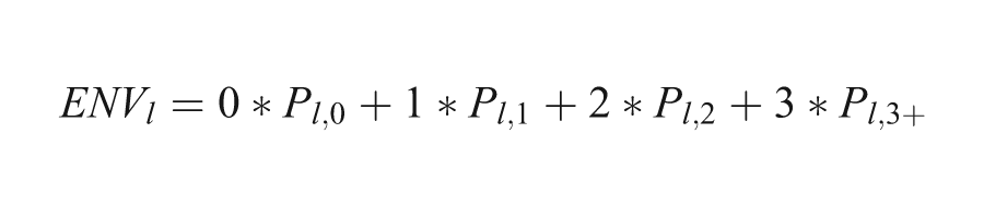
where $l$ is the household index and $P_{l, k}$ is the predicted probability of household $l$ owning $k$ vehicles (0, 1, 2, or 3+), based on the multinomial logit results. ENV was substituted for the observed number of household vehicles in travel outcome regressions.

The selectivity bias correction (SBC) factor was calculated for each household based on the results of a binary logit model of vehicle ownership. The SBC calculation took the following form (Zegras, 2010):

S B C_{l} = (\frac{1}{K}) \sum_{k \neq c}^{K} [P_{l, k} l n (P_{l, k}) / (1 - P_{l, k}) + l n (P_{l, c})]

where $l$ is the household index, $k$ is the index of alternatives (0 or 1+ vehicles), $c$ is the index of the chosen alternative, $K$ is the number of alternatives (2), and $P_{l, k}$ is the predicted probability of household $l$ owning $k$ vehicles, based on the binary logit results. We used regression to analyse factors associated with our continuous travel outcomes, including the number of daily walking trips, transit trips, and VMT. We developed two types of models: one type including ENV and SBC factors as independent variables without the number of household vehicles and one type excluding these factors and including the number of household vehicles. Since these approaches provided consistent results, we report only results for models including ENV and SBC factors. We specified negative binomial (NB) generalised linear models for daily walking trips and transit trips since these variables were count variables which were over-dispersed. We specified Tobit regression models for daily household VMT since this variable was left-censored.

Overview of samples and travel patterns

We conducted an analysis of three samples: the countywide sample including both CHTS and NTAS households (N = 8602), the combined NTAS/CHTS sample for the NTAS study area only (N = 696), and the NTAS sample alone (N = 383) (Table 1). The NTAS sample provides insights regarding socio-psychological and residential preferences based on questions that were only asked for the NTAS sample. We identified six households that seem to have responded to both the CHTS and NTAS surveys, and we excluded their CHTS responses from the combined dataset to avoid duplication.

Table 1.

Descriptive characteristics of samples.

	Countywide sample (CHTS and NTAS)	Study area sample (NTAS)
Total households	8602	383
Household characteristics
Household workers (N)	1.25	1.02
Household non-workers (N)	1.29	0.66
Children under 6 years (N)	0.11	0.07
Household vehicles (N)	1.72	1.17
Household race (at least one member)
Hispanic or Latino (1/0)	0.30	0.13
Black or African-American (1/0)	0.09	0.05
Asian or Pacific Islander (1/0)	0.11	0.17
Other (1/0)	0.15	0.07
White (1/0)	0.69	0.63
Housing type
Single family residential	0.61	0.14
Annual household income
Under $35,000	0.25	0.31
$35,000–$74,999	0.26	0.38
$75,000–$99,999	0.13	0.15
$100,000 or higher	0.26	0.14
Missing	0.10	0.01
Highest household educational attainment
Less than high school (1/0)	0.33	0.04
High school or equivalent (1/0)	0.24	0.15
Associate’s degree (1/0)	0.10	0.03
Bachelor’s degree (1/0)	0.29	0.39
Graduate degree (1/0)	0.31	0.33
Missing	0.01	0.06
Near-residence land use (< .25 mi or .4 km)
Residential (all) (%)	0.72	0.37
Commercial (all) (%)	0.09	0.19
Near-residence transit factors
Transit line stops within 1/4 mile (N)	30.83	93.51
Distance to light rail station (miles)	6.39	0.33
Near-residence built environment (< .25 mi or .4 km)
Intersections (N)	40.53	36.15
Employment, total (N)	815	2631
Population density and employment access measures
Population density (log)	9.05	9.77
Employment/destination access (EDA) (standardised)	0.44	1.39
Daily trips by mode and vehicle distance travelled
Total trips	8.27	6.33
Walk	1.37	1.61
Bus	0.34	0.49
Rail transit	0.09	0.45
Personal vehicle	6.25	3.5
Vehicle kilometres travelled (VKT)	55.86	40.99
Vehicle metres travelled (VMT)	34.71	25.47

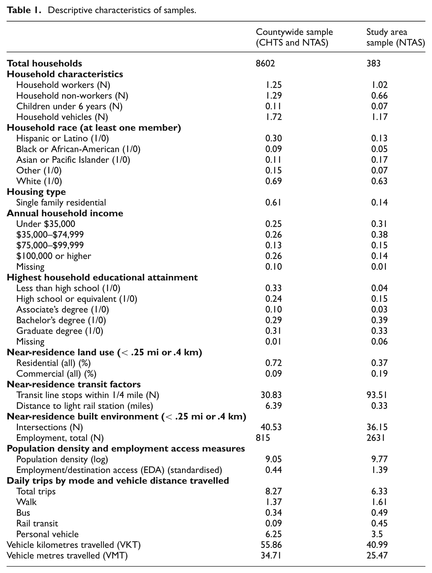
Compared to the county sample, the NTAS study area sample had fewer household members and vehicles on average, a lower percentage of households residing in a single-family residence, and higher percentages of households with an annual income under $75,000 and households with at least one member with an educational attainment of a bachelor’s degree or higher. The NTAS sample households also tended to have less nearby residential land use, more nearby commercial, and higher near-residence transit access, population density, and employment/destination access. The NTAS study area sample had fewer daily trips, fewer vehicle trips, and lower VMT than the countywide sample. Note that, for the NTAS sample VMT was estimated from household vehicle odometer logs while for the CHTS sample VMT was estimated from the reported locations of trip origins and destinations.

Factor analysis: Socio-psychological constructs

For the NTAS study area sample, one adult respondent in each household was asked to complete a questionnaire that included demographic, attitudinal, and personal safety related questions. Survey items were adapted from questions shown to affect travel behaviour and transit usage in similar studies (Anable, 2005; Heath and Gifford, 2002; Hunecke et al., 2008; Spears et al., 2013). Specifically, we asked questions related to the perceived neighbourhood amenities within walking distance of home, transit attitudes and social support, and car attachment and perceived control over travel behaviour. In all, the main respondent in each household was asked to rank 13 overlapping socio-psychological statements on a 7-point Likert scale ranging from 1 (strongly disagree) to 7 (strongly agree).

The first step in analysing participant responses to attitudinal questions was to use exploratory factor analysis to reduce the 13 questions to a smaller set of factors that could be used in regression analysis. Each factor formed through this analysis was comprised of variables that were most highly correlated with each other and least correlated with variables in other factors. Consistent with previous studies, we used principal component analysis with varimax rotation to reduce the responses to the relevant survey questions into orthogonal factors that were treated as uncorrelated variables in subsequent analysis (Anable, 2005; Heath and Gifford, 2002; Hunecke et al., 2008; Spears et al., 2013). Based on a scree plot showing the variance explained by each factor, a three factor solution was chosen for the analysis. The resulting factors explained 49.7% of the variance in the attitudinal responses. To evaluate the internal reliability of the factors, Cronbach’s alpha was calculated for each, using the variables with the highest loadings on each factor. Table 2 shows the three factors extracted from the analysis that were used as independent variables in subsequent regression analysis and Cronbach’s alpha for each factor. The table also lists the three to five statements which participants ranked from ‘strongly disagree’ to ‘strongly agree’ and which were used to construct each factor.

Table 2.

Factor analysis results.

Factor	Survey item	Factor loading	Cronbach’s α
Perceived neighbourhood amenities	There are plenty of places to shop within walking distance of my home.	0.838	0.81
There are good restaurants within walking distance of my home.	0.833
	There are enough places in my neighbourhood where I can go for recreation or entertainment.	0.784
	I can get most of my personal business (like banking, laundry, etc.) done within walking distance of my home.	0.693
Car attachment	It is/would be difficult to get everything done without a car.	0.706	0.59
	Using the bus or train takes too long compared to going by car.	0.677
	I feel pressed for time in my daily travels.	0.676
	I am uncomfortable on a crowded bus or train.	0.369
Transit attitudes and support	Increasing use of public transit is beneficial to the environment.	0.678	0.57
	Taking the bus or train could save me money compared to driving a car.	0.601
	I try to minimise my impact on the environment by taking the bus or train whenever I can.	0.578
	I don’t know enough about public transit in my neighbourhood to use it.	--0.499
	My friends and family would support me if I decided to use my car less.	0.484

Results

Analysis of vehicle ownership

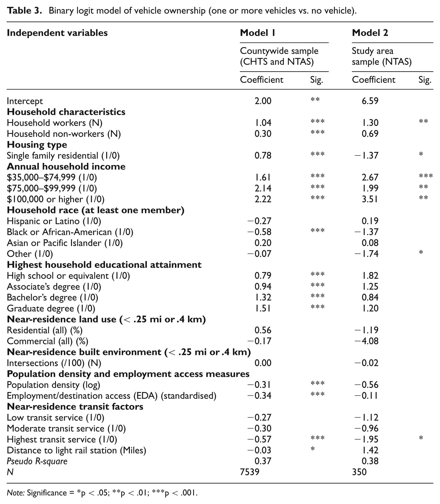
We conducted binary and multinomial logit (MNL) regression analysis to assess factors associated with household car ownership. These models assess the association of demographic, household, and near-residence built environment factors with household car ownership and will provide the basis for generating ENV factors (based on the MNL regression results) and SBC factors (based on the binary logistic regression results) which will be used as independent variables for subsequent regression models of travel outcomes. Although many socio-demographic variables were significant in the models, we focus the discussion on built environment, land use, and transit access variables since they are the most relevant to policy and the study hypotheses.

Based on the binary logistic regression models (Table 3), higher population density and employment/destination access were associated with a lower probability of vehicle ownership for both the countywide and study area sample. For both samples, having more nearby rail- and bus-transit service was associated with a lower probability of vehicle ownership, and distance to a light rail station was negatively associated with vehicle ownership for the countywide sample. These patterns are consistent with previous studies, which indicate vehicle ownership is associated with land use, density, and transit access (Bento et al., 2005; Zegras, 2010).

Table 3.

Binary logit model of vehicle ownership (one or more vehicles vs. no vehicle).

Independent variables	Model 1		Model 2
	Countywide sample (CHTS and NTAS)		Study area sample (NTAS)
	Coefficient	Sig.	Coefficient	Sig.
Intercept	2.00	**	6.59
Household characteristics
Household workers (N)	1.04	***	1.30	**
Household non-workers (N)	0.30	***	0.69
Housing type
Single family residential (1/0)	0.78	***	−1.37	*
Annual household income
$35,000–$74,999 (1/0)	1.61	***	2.67	***
$75,000–$99,999 (1/0)	2.14	***	1.99	**
$100,000 or higher (1/0)	2.22	***	3.51	**
Household race (at least one member)
Hispanic or Latino (1/0)	−0.27		0.19
Black or African-American (1/0)	−0.58	***	−1.37
Asian or Pacific Islander (1/0)	0.20		0.08
Other (1/0)	−0.07		−1.74	*
Highest household educational attainment
High school or equivalent (1/0)	0.79	***	1.82
Associate’s degree (1/0)	0.94	***	1.25
Bachelor’s degree (1/0)	1.32	***	0.84
Graduate degree (1/0)	1.51	***	1.20
Near-residence land use (< .25 mi or .4 km)
Residential (all) (%)	0.56		−1.19
Commercial (all) (%)	−0.17		−4.08
Near-residence built environment (< .25 mi or .4 km)
Intersections (/100) (N)	0.00		−0.02
Population density and employment access measures
Population density (log)	−0.31	***	−0.56
Employment/destination access (EDA) (standardised)	−0.34	***	−0.11
Near-residence transit factors
Low transit service (1/0)	−0.27		−1.12
Moderate transit service (1/0)	−0.30		−0.96
Highest transit service (1/0)	−0.57	***	−1.95	*
Distance to light rail station (Miles)	−0.03	*	1.42
Pseudo R-square	0.37		0.38
N	7539		350

Note: Significance = *p < .05; **p < .01; ***p < .001.

Although not shown, the MNL models estimated three equations: the probability that a household will own one vehicle versus no vehicle, the probability that a household will own two vehicles versus no vehicle, and the probability that a household will own three or more vehicles versus no vehicle. The signs and significance of variables in the binary regression were largely consistent with the patterns in the MNL models.

Countywide results: Factors associated with key travel outcomes

We next conducted multivariate analysis to better understand the relative influence of built environment, land use, and transit access characteristics on three categories of travel: walking travel, transit travel, and household VMT (Table 4). We report models including the ENV and SBC factors generated from the vehicle choice models (without the number of household vehicles and including only households with at least one reported vehicle), assuming that the near-residence built environment, land use, and transit access characteristics influence travel outcomes by first influencing a household’s choice of vehicle ownership.

Table 4.

Regression results for travel outcomes, countywide sample (CHTS and NTAS).

Independent variables	Model 3 (NB)		Model 4 (NB)		Model 5 (Tobit)
	Walking trips		Bus/train trips		Household VMT
	Coefficient	Sig.	Coefficient	Sig.	Coefficient	Sig.
Intercept	−1.40	**	−4.32	***	−11.55
Household travel characteristics
At least one household work trip (1/0)	0.25	***	0.84	***	20.65	***
Household composition
Household workers (N)	0.26		0.34		6.49	**
Household non-workers (N)	0.34	***	0.32	**	1.85
Children under 6 years (N)	0.03		−0.35	*	−2.51
Housing type
Single family residential (1/0)	−0.43	**	−0.35		−0.95
Household vehicle ownership
Expected number of vehicles (ENV)	0.20		−0.03		13.33	*
Annual household income
$35,000–$74,999 (1/0)	−0.63	***	−0.71	*	10.01	***
$75,000–$99,999 (1/0)	−0.60	**	−1.08	**	10.72	**
$100,000 or higher (1/0)	−0.52	*	−1.02	**	10.57	**
Household race (at least one member)
Hispanic or Latino (1/0)	0.24	**	0.76	***	2.81
Black or African-American (1/0)	0.01		0.77	***	−0.43
Asian or Pacific Islander (1/0)	−0.02		0.48	**	−1.55
Other (1/0)	0.04		−0.28		−1.58
Highest household educational attainment
High school or equivalent (1/0)	−0.32		−0.07		5.40
Associate’s degree (1/0)	−0.41		−0.06		8.42
Bachelor’s degree (1/0)	−0.12		0.08		8.21	*
Graduate degree (1/0)	0.09		0.15		10.62	*
Near-residence land use (< .25 mi or .4 km)
Residential (all) (%)	0.32		0.22		3.66
Commercial (all) (%)	0.72		0.36		10.83
Near-residence built environment (< .25 mi or .4 km)
Intersections (/100) (N)	−0.18		−0.43		−0.29
Population density and employment access measures
Population density (log)	0.03		0.14		−2.03	**
Employment/destination access (EDA) (standardised)	0.23	***	0.01		−4.08	***
Near-residence transit factors
Transit service level
Low transit service (1/0) (quartile 2)	0.11		−0.03		−3.71	*
Moderate transit service (1/0) (quartile 3)	0.20	*	0.42	*	−4.93	**
Highest transit service (1/0) (quartile 4)	0.41	***	0.55	**	−5.42	**
Distance to light rail station
0–0.5 miles (1/0)	0.38	**	1.08	***	0.41
0.5–1.0 miles (1/0)	0.16		0.67	**	−1.22
1.0–1.5 miles (1/0)	0.14		0.65	**	−1.24
1.5–2.0 miles (1/0)	0.15		0.51	*	0.91
2.0–2.5 miles (1/0)	0.05		0.25		−2.75
Flags
Selection bias correction (SBC)	0.41		0.48		−22.57	**
Dispersion	5.42		14.00
Pseudo R-square (NB) or adjusted R-square (Tobit)	0.04		0.06		0.02
N	6926		6926		6883

Note: Significance = *p < .05; **p < .01; ***p < .001. NB = negative binomial regression.

Regression results for the countywide sample show that near-residence employment/destination access was associated with a greater number of walking trips and that population density and employment/destination access were associated with lower household VMT. Households in the highest two quartiles of transit service were associated with more walking and transit trips and lower household VMT. Households within 0.5 miles (0.8 km) of a rail transit station were associated with more walking trips and households within 2.0 miles (3.2 km) of a rail transit station were associated with more transit trips. Overall, the countywide models explained only about 2–6% of the variance in daily household walking trips, transit trips, and VMT, suggesting unobserved factors may have an important influence on these outcomes.

Rail transit corridor results: Factors associated with key travel outcomes

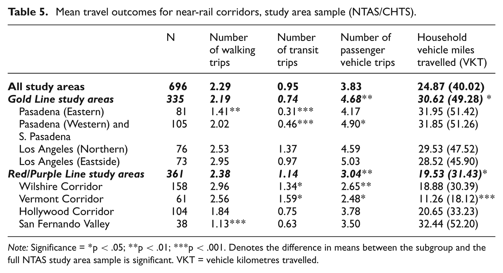
We replicated our travel outcome models for households in the NTAS study area to better understand variations in built environment–travel relationships within policy-relevant rail transit corridors. For the combined NTAS/CHTS sample for the study area, participating households near the Gold Line were not significantly different from participating households near the Red/Purple Line in terms of overall walking and transit travel, but households near the Gold Line had significantly more vehicle trips and VMT (Table 5). Households in the Wilshire and Vermont segments of the Red/Purple Line had significantly more transit travel and significantly fewer vehicle trips. The Vermont segment had significantly lower VMT than all households in the NTAS study area.

Table 5.

Mean travel outcomes for near-rail corridors, study area sample (NTAS/CHTS).

	N	Number of walking trips	Number of transittrips	Number of passenger vehicle trips	Household vehicle miles travelled (VKT)
All study areas	696	2.29	0.95	3.83	24.87 (40.02)
Gold Line study areas	335	2.19	0.74	4.68**	30.62 (49.28) *
Pasadena (Eastern)	81	1.41**	0.31***	4.17	31.95 (51.42)
Pasadena (Western) and S. Pasadena	105	2.02	0.46***	4.90*	31.85 (51.26)
Los Angeles (Northern)	76	2.53	1.37	4.59	29.53 (47.52)
Los Angeles (Eastside)	73	2.95	0.97	5.03	28.52 (45.90)
Red/Purple Line study areas	361	2.38	1.14	3.04**	19.53 (31.43)*
Wilshire Corridor	158	2.96	1.34*	2.65**	18.88 (30.39)
Vermont Corridor	61	2.56	1.59*	2.48*	11.26 (18.12)***
Hollywood Corridor	104	1.84	0.75	3.78	20.65 (33.23)
San Fernando Valley	38	1.13***	0.63	3.50	32.44 (52.20)

Note: Significance = *p < .05; **p < .01; ***p < .001. Denotes the difference in means between the subgroup and the full NTAS study area sample is significant. VKT = vehicle kilometres travelled.

We developed a model for each of the travel outcomes (walking trips, transit trips, and VMT) for the NTAS rail corridor sample using the explanatory factors previously used in the countywide models (Table 4), corridor dummy variables to assess potential differences across corridors, and socio-psychological and neighbourhood preference factors (were not available for the CHTS countywide sample). The percentage of nearby residential land uses was positively associated with fewer transit trips, and the percentage of nearby commercial land uses was associated with higher VMT. In contrast to countywide models, results for the NTAS sample indicate that after controlling for household and socio-demographic factors, nearby population density and employment/destination accessibility were not significantly associated with the three travel outcomes (Table 6). Higher nearby transit service level was not significantly associated with travel patterns. These unexpected results may be due to the lower variation in transit access and population density within the study corridors compared to the county as a whole. For instance, the population density near NTAS households was on average about twice that near countywide sample households, and about 98% of NTAS households were located within 0.25 miles of at least one transit stop compared to about 79% of the countywide sample.

Table 6.

Regression results for travel outcomes, study area sample (NTAS).

Independent variables	Model 6 (NB)		Model 7 (NB)		Model 8 (Tobit)
	Walking trips		Bus/train trips		Household VMT
	Coef.	Sig.	Coef.	Sig.	Coef.	Sig.
Intercept	--0.89		--1.69		--93.29	*
Household travel characteristics
At least one household work trip (1/0)	--0.29		0.04		--5.91
Household composition
Household workers (N)	1.22	**	1.58	***	6.92
Household non-workers (N)	0.51	*	1.07	***	--5.99
Children under 6 years (N)	--0.36		--1.75		0.52
Housing type
Single family residential (1/0)	--0.27		1.01		2.55
Household vehicle ownership
Expected number of vehicles (ENV)	--0.66		--3.22	*	27.45	*
Annual household income
$35,000–$74,999 (1/0)	0.44		1.67	**	--2.55
$75,000–$99,999 (1/0)	0.20		1.57	*	0.79
$100,000 or higher (1/0)	0.39		1.11		1.43
Household race (at least one member)
Hispanic or Latino (1/0)	0.34		0.39		1.32
Black or African-American (1/0)	--1.41		--1.50		14.87
Asian or Pacific Islander (1/0)	--0.72	*	--0.10		--6.24
Other (1/0)	--0.33		--1.40		14.35
Highest household educational attainment
Associates or Bachelor’s degree (1/0)	0.09		--0.19		3.18
Graduate degree (1/0)	0.02		0.29		7.38
Near-residence land use (< .25 mi or .4 km)
Residential (all) (%)	2.30		--3.73	*	12.18
Commercial (all) (%)	0.56		--3.66		103.32	**
Near-residence built environment (< .25 mi or .4 km)
Intersections (/100) (N)	0.04		2.11	*	11.16
Population density and employment access measures
Population density (log)	--0.15		0.28		5.42
Employment/destination access (EDA) (standardised)	0.39		--0.83		5.46
Near-residence transit factors
Transit service level (line-stops/100)	0.03		--0.15		--1.80
Distance to light rail station (miles)	0.29		0.07		23.61
Red/Purple Line study areas
Wilshire Corridor (1/0)	--0.40		0.81		--22.28	*
Vermont Corridor (1/0)	--0.43		1.29	*	--27.81	**
Hollywood Corridor (1/0)	--0.43		0.13		--12.54
San Fernando Valley (1/0)	0.03		--0.50		8.78
Socio-psychological constructs, main respondent
Perceived neighbourhood amenities	0.36	*	0.32		--2.82
Perceived need for a car	--0.32	*	--0.76	***	4.69
Transit attitudes and transit social norms	0.35	**	0.80	***	0.37
Neighbourhood preference, main respondent
Access to job	0.31		--0.90	**	--12.99	**
Access to transit	0.34		1.24	***	--14.67	*
Access to highway	--0.68		--0.58		9.34
Flags
Selection bias correction (SBC)	--0.90		1.06		--9.85
Dispersion	2.14		0.89
Pseudo R-square (NB) or adjusted R-square (Tobit)	0.08		0.23		0.04
N	286		286		286

Note: Significance = *p < .05; **p < .01; ***p < .001. NB = negative binomial regression.

When we specified these models using only the explanatory factors previously used in the countywide models, the models only explained about 2–8% of the variance in the travel outcomes. When we added rail corridor dummy variables to assess potential differences across corridors, the explained variance for the models increased only slightly. In the full models, corridor flags were not significant in the walking trips model (Model 6), but households in the Vermont segment of the Red/Purple Line were associated with more transit trips than households along the Gold Line (the excluded category) (Model 7). Study households residing in the Vermont or Wilshire segments of the Red/Purple Line were associated with lower VMT (Model 8).

The addition of socio-psychological constructs (described in Table 2) and neighbourhood preference factors increased the explanatory power of the models over the model iterations including corridor flags, by 4%, 15%, and 1% respectively for walking trips, transit trips, and VMT. Households with a main respondent who had positive transit attitudes (e.g. felt transit use benefits the environment and saves money) were associated with more walking. Those with stronger car attachment (e.g. felt getting daily tasks done without a car would be difficult, felt bus or train takes too long) were associated with less walking and transit usage. After controlling for more ‘objective’ measures of the built environment, land use, and transit service, our measure of participant perceived neighbourhood amenities (e.g. shopping and restaurants within walking distance) was associated with more walking trips. Neighbourhood preference factors were not significantly associated with walking behaviour after controlling for other factors, but households with a main respondent who indicated that access to his or her job was ‘extremely important’ during their last move were associated with fewer transit trips and lower VMT. Those who indicated access to transit was ‘extremely important’ during their last move were associated with more transit trips and lower VMT.

Discussion

Results for the countywide sample are consistent with previous research suggesting that, after controlling for household socio-demographic factors and income, areas with higher population density, greater employment/destination access, and higher transit service are associated with lower vehicle ownership and usage. Households within 0.5–2.0 miles (0.8–3.2 km) of a rail transit station tended to have more walking and transit trips, and these relationships were strongest for households within 0.5 miles (0.8 km) of a rail transit station. These patterns suggest that efforts to target household and job growth in dense, high quality transit areas in the region may support policy goals to reduce household vehicle travel and promote greater transit usage and walking.

Although distance to a rail transit station was associated with reduced household VMT for the countywide sample, we found substantial variation in the travel patterns across rail corridor segments. On average, households along the Red/Purple Line had about 11 fewer daily miles (18 km) driven and more transit ridership than households along the Gold Line. This pattern was strongest for households in the Wilshire and Vermont segments of the Red/Purple Line, which were among the densest rail transit segments analysed. Interestingly, the variables controlling for population density and employment/destination access in our regression analyses were insignificant regardless of whether we included corridor dummy variables in the models, which seems to indicate that unobserved factors within these corridors could be having an important influence on travel outcomes.

One possible explanation for why households along the Wilshire and Vermont segments of the Red/Purple Line had much higher transit usage and much lower VMT may be development patterns. These segments are the oldest rail segments in Los Angeles Metro’s transit network, and they have substantial completed TOD investment, some of which was supported by Metro’s joint development programme, which seeks private and/or public sector partnerships to develop on Metro-owned property at and adjacent to transit stations. Although several large developments have been completed along the Gold Line and several are in predevelopment or construction, especially on the East Los Angeles segment, more time is needed for development along its segments to come to fruition and potentially influence behaviour (Loukaitou-Sideris, 2010). Our results suggest that rail transit corridors are not created equally and stress the importance for transit providers and community planners to understand that the ability of near-transit compact growth to reduce vehicle travel could vary substantially depending on station area neighbourhood constraints and development context.

Despite efforts by the region’s planning organisations to direct over half of household and employment growth by 2035 towards transit corridors, public debates continue regarding the character and intensity of near-rail development and have intensified as the Los Angeles Planning Department seeks to align community land use plans with regional goals. For example, a major focus of the update to the Hollywood Community Plan, adopted in 2012, was to direct density and orient neighbourhoods towards the Red Line, and substantial public concern focused on how to foster transit-supportive densities while preserving established single-family neighbourhoods (City of Los Angeles Department of City Planning, 2012). Similar debate has emerged as the city initiates workshops to update the Boyle Heights Community Plan; the neighbourhood council and community groups have raised concerns that increased development along the Gold Line will trigger gentrification and displacement of residents of this largely low-income, Latino neighbourhood.

Another plausible explanation for why households along the older segments of the Red/Purple Line had much higher transit usage and lower VMT may be the composition, attitudes, and preferences of their residents. Consistent with previous research suggesting that these factors play an important role in transit ridership and lower vehicle usage (Cao et al., 2009; Cervero, 2007; Næss, 2006), the addition of socio-psychological and residential preference factors strengthened the explanatory power of our travel outcome models for the NTAS near-rail supplemental sample. This suggests transit providers and community planners should not only focus on improving transit access and maximising development in rail corridors, but also tailor policies to account for perceptions, attitudes and residential preferences. Previous research indicates programmes that include personalised travel planning, transit information marketing programmes, and travel awareness campaigns tailored to address socio-psychological barriers to transit use could result in increased trips taken by non-car modes (Moser and Bamberg, 2008). Further research is needed to understand the influence of station-area socio-demographic and economic context on whether nearby residents change their travel behaviour and the extent to which new households move near stations because they prefer to reside in denser, more walkable, and mixed-use communities with greater transit access. Our findings suggest that directing growth towards compact rail corridors could play an important role in transforming the automobile city, but we find substantial variation in travel patterns and the development context within rail corridors. Future regional travel surveys should seek sizeable samples across a diversity of rail transit corridors in order to better understand how near-rail land use–travel interactions diverge across corridors and from countywide patterns and should collect information on socio-psychological and neighbourhood preference factors. Evaluation studies are also needed to assess whether rail transit investments encourage long-term corridor residents to shift towards more sustainable modes and to better understand the role of gentrification, residential displacement, and the movement of new residents to rail transit corridors. A recent before-and-after quasi-experimental evaluation of the impact of the Expo Line light rail in Los Angeles found that households within a half-mile of the new service travelled on average about 10–12 miles less per day by car after the new service began, which was associated with about a 30% reduction in vehicle carbon emissions (Boarnet et al., 2013). In addition to project evaluation, ongoing monitoring is needed to assess the implementation and impact of regional plans seeking to direct sizeable employment and housing growth into communities with high quality transit service. These studies should consider the relative importance of other factors which could influence sustainable travel and emissions reductions including demand management, technological improvements, near-station parking availability, gas prices and fares, and differences across bus and rail riders (Brown et al., 2014; Chatman, 2013; Chen et al., 2011).

Footnotes

Funding

This research was supported by the California Department of Transportation and the University of California Multi-Campus Research Program on Sustainable Transportation.

References

Anable

(2005) ‘Complacent car addicts’ or ‘aspiring environmentalists’? Identifying travel behaviour segments using attitude theory. Transport Policy 12(1): 65–78.

Arvidsson

Kawakami

Ohlsson

. (2012) Physical activity and concordance between objective and perceived walkability. Medicine and Science in Sports and Exercise 44(2): 280–287.

Bamberg

Ajzen

Schmidt

(2003) Choice of travel mode in the theory of planned behavior: The roles of past behavior, habit, and reasoned action. Basic and Applied Social Psychology 25: 175–188.

Barbour

Deakin

(2012) Smart growth planning for climate protection. Journal of the American Planning Association 78(1): 70–86.

Bento

Cropper

Mobarak

. (2005) The impact of urban spatial structure on travel demand in the United States. The Review of Economics and Statistics 87(3): 466–478.

Boarnet

Hong

Lee

. (2013) The Exposition Light Rail Line Study: A Before-and-After Study of the Impact of New Light Rail Transit Service. Los Angeles: Haynes Foundation.

Boarnet

Houston

Ferguson

. (2011) Land use and vehicle miles of travel in the climate change debate: Getting smarter than your average bear. In: Ingram

Hong

Y-H

(eds) Climate Change and Land Policies. Cambridge, MA: Lincoln Institute of Land Policy, pp. 151–187.

Boarnet

Joh

Siembab

. (2011) Retrofitting the suburbs to increase walking: Evidence from a land use–travel study. Urban Studies 48(1): 129–159.

Brown

Werner

(2008) Before and after a new light rail stop: Resident attitudes, travel behavior, and obesity. Journal of the American Planning Association 75(1): 5–12.

10.

Brown

Thompson

Bhattacharya

. (2014) Understanding transit ridership demand for the multidestination, multimodal transit network in Atlanta, Georgia: Lessons for increasing rail transit choice ridership while maintaining transit dependent bus ridership. Urban Studies 51(5): 938–958.

11.

Brownstone

Golob

(2009) The impact of residential density on vehicle usage and energy consumption Journal of Urban Economics 65(1): 91–98.

12.

California Department of Transportation (2013) 2010–2012 California household travel survey final report. Report. Sacramento, CA: California Department of Transportation.

13.

Cao

Mokhtarian

Handy

(2009) Examining the impacts of residential self-selection on travel behaviour: A focus on empirical findings. Transport Reviews 29(3): 359–395.

14.

Cervero

(1993) Ridership impacts of transit-focused development in California. Working paper no. 176, University of California Transportation Center, University of California, Berkeley, CA, USA.

15.

Cervero

(2007) Transit oriented development’s ridership bonus: A product of self-selection and public policies. Environment and Planning Part A 39(9): 2068–2085.

16.

Cervero

Murakami

(2010) Effects of built environments on vehicle miles traveled: Evidence from 370 US urbanized areas. Environment and Planning A 42(2): 400–418.

17.

Cervero

Ferrell

Murphy

(2002) Transit-oriented development and joint development in the United States: A literature review. Report 52, Transportation Cooperative Research Program, Washington, DC, October.

18.

Chatman

(2008) Deconstructing development density: Quality, quantity and price effects on household non-work travel. Transportation Research Part A: Policy and Practice 42(7): 1008–1030.

19.

Chatman

(2013) Does TOD need the T? Journal of the American Planning Association 79(1): 17–31.

20.

Chen

Varley

Chen

(2011) What affects transit ridership? A dynamic analysis involving multiple factors, lags and asymmetric behaviour. Urban Studies 48: 1893–1908.

21.

City of Los Angeles Department of City Planning (2012) Hollywood Community Plan. Los Angeles: City of Los Angeles Department of City Planning.

22.

Dierwechter

Wessells

(2013) The uneven localisation of climate action in metropolitan Seattle. Urban Studies 50: 1368–1385.

23.

Ewing

Cervero

(2010) Travel and the built environment: A meta analysis. Journal of American Planning Association 76(3): 265–294.

24.

Forsyth

Hearst

Oakes

. (2008) Design and destinations: Factors influencing walking and total physical activity. Urban Studies 45: 1973–1996.

25.

Forsyth

Oakes

Schmitz

. (2007) Does residential density increase walking and other physical activity? Urban Studies 44(4): 679–697.

26.

Gebel

Bauman

Sugiyama

. (2011) Mismatch between perceived and objectively assessed neighborhood walkability attributes: Prospective relationships with walking and weight gain. Health and Place 17(2): 519–524.

27.

Guerra

Cervero

Tischler

(2012) Half-mile circle does it best represent transit station catchments? Journal of the Transportation Research Board 2276: 101–109.

28.

Handy

(2005) Critical assessment of the literature on the relationships among transportation, land use and physical activity. Report for the Transportation Research Board. Report no. 282, January. Washington, DC: Transportation Research Board.

29.

Heath

Gifford

(2002) Extending the theory of planned behavior: Predicting the use of public transportation. Journal of Applied Social Psychology 32(10): 2154–2189.

30.

Holden

Linnerud

(2011) Troublesome leisure travel: The contradictions of three sustainable transport policies. Urban Studies 48(14): 3087–3106.

31.

Hunecke

Haustein

Bohler

. (2008) Attitude-based target groups to reduce the ecological impact of daily mobility behavior. Environment and Behavior 42(1): 3–43.

32.

Joh

Nguyen

Boarnet

(2012) Can built and social environmental factors encourage walking among individuals with negative walking attitudes? Journal of Planning Education and Research 32(2): 219–236.

33.

Kuby

Barranda

Upchurch

(2004) Factors influencing light-rail station boardings in the United States. Transportation Research A 38(3): 223–258.

34.

Loo

BPY

Chen

Chan

ETH

(2010) Rail-based transit-oriented development: Lessons from New York City and Hong Kong. Landscape and Urban Planning 97: 202–212.

35.

Los Angeles Metropolitan Transportation Authority (2009) Long Range Transportation Plan. Los Angeles: Los Angeles Metropolitan Transportation Authority.

36.

Loukaitou-Sideris

(2010) A new-found popularity for transit-oriented developments? Lessons from Southern California. Journal of Urban Design 15(1): 49–68.

37.

Lund

(2006) Reasons for living in a transit-oriented development, and associated transit use. Journal of the American Planning Association 72: 357–366.

38.

Lund

Cervero

Wilson

(2004) Travel characteristics of transit-oriented development in California. Report, January. Sacramento, CA: California Department of Transportation.

39.

Mannering

(1986) Selectivity bias in models of discrete and continuous choice: An empirical analysis. Transportation Research Record 1085: 58–62.

40.

Millward

Spinney

Scott

(2013) Active-transport walking behavior: Destinations, durations, distances. Journal of Transport Geography 28: 101–110.

41.

Moser

Bamberg

(2008) The effectiveness of soft transport policy measures: A critical assessment and meta-analysis of empirical evidence. Journal of Environmental Psychology 28(1): 10–26.

42.

Næss

(2006) Accessibility, activity participation and location of activities: Exploring the links between residential location and travel behaviour. Urban Studies 43(3): 627–652.

43.

Ong

Graham

Houston

(2006) The policy and programmatic importance of spatial alignment of multiple GIS data sources. American Journal of Public Health 96: 499–504.

44.

Saelens

Handy

(2008) Built environment correlates of walking: A review. Medicine and Science in Sports and Exercise 40(7 Suppl): S550–S566.

45.

Salon

Boarnet

Handy

. (2012) How do local actions affect VMT? A critical review of the empirical evidence. Transportation Research Part D 17: 495–508.

46.

Southern California Association of Governments (2012) 2012–2035 regional transportation plan. Los Angeles: Southern California Association of Governments. Available at: http://rtpscs.scag.ca.gov/Pages/default.aspx.

47.

Spears

Houston

Boarnet

(2013) Illuminating the unseen in transit use: A framework for examining the effect of attitudes and perceptions on travel behavior. Transportation Research Part A: Policy and Practice 58: 40–53.

48.

Taylor

Miller

Iseki

. (2009) Nature and/or nurture? Analyzing the determinants of transit ridership across US urbanized areas. Transportation Research Part A: Policy and Practice 43: 60–77.

49.

Thompson

Brown

Bhattacharya

(2012) What really matters for increasing transit ridership: Understanding the determinants of transit ridership demand in Broward County, Florida. Urban Studies 49: 3327–3345.

50.

Van Acker

Van Wee

Witlox

(2010) When transport geography meets social psychology: Toward a conceptual model of travel behaviour. Transport Reviews 30(2): 219–240.

51.

Zegras

(2010) The built environment and motor vehicle ownership and use: Evidence from Santiago de Chile. Urban Studies 47(8): 1793–1817.