Synchronisation and commonalities in metropolitan housing market cycles

Abstract

This paper examines the degree of commonalities present in the cyclical behaviour of the eight largest metropolitan housing markets in Australia. Using two techniques originally proposed in the business cycle literature we firstly consider the degree of synchronisation present and secondly decompose the series into their permanent and cyclical components. Both empirical approaches reveal similar results. Sydney and Melbourne are closely related to each other and are relatively segmented from the smaller metropolitan areas. In contrast, there is substantial evidence of commonalities in the cyclical behaviour of the remaining cities, especially those on the eastern and southern coasts of Australia.

Keywords

common cycles decomposing cycles and trends house price diffusion metropolitan housing markets permanent and transitory components

Introduction

Over the course of the last two decades a large literature has developed to have considered the interaction and relationships present amongst either metropolitan or regional housing markets. In the main this has considered the issue from the perspective of house price diffusion and the analysis of whether causal relationships exist. This literature is particularly prevalent in the UK where considerable research has been conducted examining the ripple effect which considers whether house prices movements in London and South East England impact upon subsequent market behaviour in the rest of the UK (e.g. Cook, 2003; Holly et al., 2011; Meen, 1999). This paper contributes to the literature by complementing the existing work on house price diffusion through the adoption of an alternative methodological framework in the context of eight metropolitan areas in Australia. We consider the capitals of Australia’s six states, namely: Adelaide (South Australia), Brisbane (Queensland), Hobart (Tasmania), Melbourne (Victoria), Perth (Western Australia) and Sydney (New South Wales). In addition to the six state capitals we also analyse Canberra (Australian Capital Territory) and Darwin (Northern Territory).

The case of Australia provides an interesting counterpoint to the studies of the UK and US. Whilst smaller in population than the UK, the geographic size of Australia is similar to the US. Because the Australian population is spread across such a wide geographic area, unlike the UK, it could be suggested that differences in the locally based economic driving forces might be more reflective of house price movements, particularly in the more geographically isolated capital cities. Therefore, the extent to which this small number of isolated metropolitan areas may display similarities in cyclical behaviour, given that they are separated by considerable distances, is interesting.

This paper considers the degree to which the primary metropolitan housing markets display characteristics that indicate the presence of common cycles. Two alternative methodological approaches are utilised in this study. The first considers the degree of synchronisation between the metropolitan markets using the modified Concordance Indicator of Harding and Pagan (2006). This approach estimates the degree to which two markets are synchronised in terms of the phase of their cycle, that is, house price appreciation or depreciation. This approach therefore provides a compliment to the conventional comparative analysis of markets. The second approach is also based upon the business cycle literature and decomposes the housing data examined into their trend and cyclical components. Two alternative decomposition approaches are considered, namely those of Beveridge and Nelson (1981) and Hodrick and Prescott (1997). The remainder of the paper is structured as follows. The next section discusses the relevant literature pertaining to the inter-linkages between housing markets. Following that, we provide information concerning the data utilised in the paper. The next two sections present and report upon the empirical findings, whilst concluding comments are made in the final section.

Literature review

The literature to have considered the interactions amongst housing markets has largely done so from the context of examining house price diffusion. A large proportion of this literature has investigated either the UK or US and to some degree, and of obvious interest in the context of the current paper, Australia.¹ The UK literature has often specifically considered the ripple effect. Meen and Andrew (1998) highlight five factors that may contribute to the presence of a ripple effect in the UK, namely: migration, transaction and search costs, equity transfer, spatial arbitrage and leads and lags in house prices. The majority of the earlier studies relied heavily upon a causality framework. For example, Giussani and Hadjimatheou (1991) and MacDonald and Taylor (1993) both report evidence supportive of the ripple effect with London as the base region. Whilst reporting broadly similar findings, the paper of Alexander and Barrow (1994) extends the analysis in two respects. Firstly, it uses the more robust Vector Error Correction Mechanism (VECM) framework. Secondly, rather than base their analysis on the premise of London being the base region, the paper considers the surrounding South East as an alternative, finding that it is actually a more appropriate base.² Muellbauer and Murphy (1994) report complementary evidence in this respect, noting that regions contiguous to the South East of England are affected not only by house price movements but also by income in the region. This can be taken as supportive of the role of spatial lags in the ripple effect.

In addition to the tests for causality, a number of papers have considered whether UK regions are cointegrated, that is, if they share a common long-term trend. MacDonald and Taylor (1993) use the bivariate Engle-Granger cointegration test, reporting significant results with respect to pairings of southern and non-southern regions.³ Cook (2005a) expands upon these tests through the adoption of cointegration tests that allow for asymmetric adjustment. The findings reported indicate that when house prices in the South of England decline relative to other regions, then reversion to equilibrium occurs quite rapidly. However, when the reverse scenario is considered, that is, prices in the south increase on a relative basis, the degree of reversion to equilibrium observed is slower.⁴

Papers in the last decade have however taken different methodological approaches to the examination of diffusion and the inter-linkages across markets. Following the observation of Meen (1999), that if the ratio of regional house prices to the overall national figure exhibits evidence of stationarity then this implies long-term convergence, a number of papers have used unit root tests to consider the issue of convergence. Two papers by Cook (2003, 2005b) test for stationarity using a variety of unit root approaches. Cook (2003) considers an asymmetric unit root specification, whilst Cook (2005b) uses the Generalised Least Squares variation of the Augmented Dickey-Fuller unit root test, as proposed by Elliot et al. (1996). The results in both papers provide evidence of convergence. In the case of Cook (2005b) significant results are reported with respect to six UK regions (North, North West, East Anglia, South East, Wales and Northern Ireland). Holmes (2007) considers the issue of stationarity in a panel setting, this complementing the work of Cook (2005b). The results indicate that converging behaviour is present in the UK regional markets.⁵ Holmes and Grimes (2008) also consider stationarity but in a slightly different context in that they firstly use principal components analysis to identify the linear combination of the regional house price series that captures the highest degree of variation across the series. They then test for stationarity in this first principal component. Holmes and Grimes (2008) find evidence of stationarity, indicating that UK regional house prices have a single common stochastic trend. A recent paper by Holmes et al. (2011) considers an aspect of specific interest in the context of the current study. The authors use a pair-wise framework to consider convergence across US markets. The approach incorporates distance and supports previous work in illustrating the importance of contiguous and non-contiguous areas. Holly et al. (2011) show that London’s global role adds an international element to house price diffusion in the UK. Whilst the results support the previously observed ripple effect, it is also noted that London is significantly linked to other global cities, in this case New York. The modelling approach adopted by Holly et al. (2011) allows it to be observed that whilst a shock to London dissipates relatively quickly (two years), the impact of such a shock to other UK regions is not only extended in a temporal sense but varies depending upon the spatial distance of the region to London.

In contrast to the UK, where the literature has largely been concerned with regional housing markets, much of the international literature has studied either metropolitan or sub-market data. In the US the early house price diffusion literature generally concentrated on diffusion between neighbouring markets, often finding results highlighting the importance of geographic proximity (e.g. Clapp and Tirtiroglu, 1994; Pollakowski and Ray, 1997).⁶ The divergence in findings between contiguous and non-contiguous markets is often attributed to factors such as the transfer of information and a positive feedback effect, whereby positive or negative movements in one market have a knock-on effect in neighbouring markets. A recent paper by Gupta and Miller (2012) considers the issue of diffusion in the case of eight metropolitan markets in Southern California, reporting substantial evidence of cointegration and causal relations across the various metropolitan markets.⁷

The distinct differences between the UK and US housing markets make an investigation of the relationships between housing markets in Australia interesting in several aspects. Similar to the UK and South East England, the southeastern corner of Australia (Sydney and Melbourne) represents a relatively large proportion of the urban population in the country. The states of New South Wales and Victoria combined represent over 58.6% of the total population of Australia and approximately 53.2% of GDP (Australian Bureau of Statistics, 2012). The urban areas of Melbourne and Sydney alone account for approximately 37.9% of the total population of Australia while the top five urban concentrations account for 59.6% of the total population, with Brisbane, Perth and Adelaide all being significantly smaller than Sydney and Melbourne (Australian Bureau of Statistics, 2012). In addition to the vast distances between the cities, the scale and relative importance of the cities within the Australian context cannot be minimised. For example, the combined populations of Brisbane, Perth and Adelaide (approximately 5.02 million) are only slightly larger than Metropolitan Sydney (approximately 4.63 million). Provided the distance and economic influences that UK results indicate in relation to London (and South East England), the increased spatial dimension and potentially varying economic fundamental variables at play in Australia provide an interesting backdrop for investigating regional variations and cyclical commonalities in house prices.

The economic characteristics of each Australian state and their respective capital cities are also reflective of the vast geographic diversity of the country. Financial services and insurance sectors hold a relatively large share of economic activity in both New South Wales and Victoria when compared with other states. The agricultural and fishing sectors both represent a relatively large increasing proportion of economic activity when examining Queensland and South Australia. In the case of Western Australia and Northern Territory, mining and natural resources hold the largest share of economic activity in those regions. For Tasmania, the forestry and fishing sectors are important economic growth drivers with government sector employment representing most of the economy in the Australian Capital Territory (Australian Bureau of Statistics, 2011).

As with many global housing markets a number of papers have recently examined the dynamics of the Australian market and in particular the degree to which speculative behaviour has possibly developed (e.g. Fry et al., 2010; Hatzvi and Otto, 2008).⁸ Costello et al. (2011) not only considered the degree of divergence from prices that can be justified according to fundamentals, but also the regional variation in such behaviour. Costello et al. (2011) note that the degree of divergence from fundamentals differs across Australian states, for example finding that whilst some states, such as Victoria, have largely seen prices in line with fundamentals since 2005, others have not. In addition, the paper considers the spill-over effect of ‘non-fundamental prices’. As with their initial analysis they report differences across states, with house prices in New South Wales most vulnerable to non-fundamental, or speculative, spill-over effects. In more conventional tests both Tu (2000) and Luo et al. (2007) consider the degree of house price diffusion present. Both papers note a number of significant results with respect to pairings of Australian markets being cointegrated. In addition, evidence of diffusion in a Granger Causality sense is also noted. This is especially evident when Sydney and Melbourne are considered. Luo et al. (2007) provide evidence that there is a distinct diffusion impact, with house price changes originating in Sydney then descending through Melbourne and subsequently to other markets. Evidence of cointegration, in a bilateral context, between a large number of Australian markets is reported. However, it would appear that Sydney, and to a lesser degree Melbourne, are again separated from the other metropolitan markets. Whilst a large number of significant results were noted, there was a marked reduction in the number when Sydney and Melbourne were examined. Sydney was only found to be cointegrated with Melbourne, whilst Melbourne added Adelaide and Perth. This can be taken as being supportive of a diffusion effect, similar to that observed in the UK, with Sydney, and then Melbourne, as the base regions.⁹

Data

The data used in this study consist of the quarterly Australian Bureau of Statistics (ABS) indices for the eight Australian capital cities, namely: Adelaide (South Australia), Brisbane (Queensland), Canberra (ACT), Darwin (Northern Territory), Hobart (Tasmania), Melbourne (Victoria), Perth (Western Australia) and Sydney (New South Wales). The data analysed cover the period June 1986 to December 2010. The indices used are not either mix-adjusted or formal hedonic indices, rather they are estimated using a weighted average approach, in common with some of the house prices indices available for the UK. A stratified clustering approach is adopted in their estimation. The weights used in the construction of the indices were re-calibrated in 2005 and the indices were correspondingly re-estimated. The re-estimated indices were retrospectively re-estimated back to 2002. We therefore use the revised indices from 2002 onwards. These were combined with the original indices, using the quarterly percentage changes, to provide continuous series dating back prior to 2002 from 1986. Figure 1 displays the constructed index series for the different markets and for the overall index, whilst the summary statistics are reported in Table 1.

Figure 1.

ABS house price indices.

Table 1.

Summary statistics.

	Average return	Standard deviation	Augmented Dickey-Fuller unit root tests
			Levels	First difference
Sydney	1.7357	2.8827	−1.8711	−4.2313***
Melbourne	1.9104	3.0254	0.7279	−4.5345***
Brisbane	1.8995	2.6287	−1.4258	−3.9443***
Adelaide	1.4637	2.3662	0.8776	−7.0731***
Perth	1.9618	2.9891	−0.6164	−3.9399***
Hobart	1.6353	2.7359	−0.2429	−3.4625**
Darwin	1.7422	2.5424	0.5383	−4.8206***
Canberra	1.6266	2.4625	−0.3992	−5.0733***
8 Capital Cities	1.7793	2.2114	−1.1178	−3.9206***

Note: Table 1 details the summary statistics for the different markets examined; ** = significance at the 5% level, and *** = significance at the 1% level.

It can be seen from Figure 1 and Table 1 that while the different markets display broad similarities in terms of their cyclical behaviour there are distinct differences also evident. Adelaide displays both a lower average quarterly return and standard deviation than the other metropolitan markets, whilst at the other extreme the city that displays both the highest return and volatility is Melbourne. In addition, the relative performance of the cities does diverge in the post 2002 period. In particular, Sydney has observed far lower price appreciation than the other markets; indeed the strongest performing markets over the course of the last decade are the smaller secondary markets such as Darwin. Table 1 also reports tests of stationarity, based upon the Augmented Dickey-Fuller test. In each case the first differenced return series is stationary.

Synchronisation of cycles

In order to consider the degree of synchronisation present in the markets considered we adopt the concordance indicator proposed by Harding and Pagan (2001, 2002, 2006) which has been utilised in a large number of papers that have considered business cycles (e.g. Altavilla, 2004; Harding and Pagan, 2001, 2002) and also in a recent paper considering the commercial office market (Jackson et al., 2008). The methodology defines state variables that consider whether a market is in a state of expansion or contraction. Harding and Pagan (2002) propose a non-parametric approach to estimating the level of concordance between two series. The growth rates are expressed as two binary random variables, S_it and S_jt , which are the state variables for cycles for markets i and j. The state variables are defined as dummy variables equalling unity when the cycle is on an upward trend and zero otherwise. Using these two state variables, the index of concordance between two cities indicates the proportion of time two cycles spend in the same phase. The concordance index can be estimated as follows:

IC = T^{- 1} \sum_{t = 1}^{T} {S_{jt} S_{it} + (1 - S_{jt}) (1 - S_{it})}

(1)

For the purposes of the state variables we define an upward trend as a positive return and a negative return as a contraction. It is important to note that the tests are considering the phase of the cycle, rather than defining a cycle itself.¹⁰ This statistic can also be adapted in what has been referred to as the Mean Corrected Index of Concordance. This adaptation, proposed by Harding and Pagan (2001), is designed to adjust the initial indicator for potential biases. Harding and Pagan (2001) noted that the original IC measure might be overstated in the case of two variables that experience prolonged expansion during the period of study. Prolonged growth over a number of consecutive periods is a common feature of real estate and economic cycles’ data. Therefore, the Mean Corrected Measure of IC (MCIC) is proposed under the assumption of no relation between two series. In comparison with the original IC statistic, the MCIC measures the proportion of time that two series are expected to share in the same phase under an assumption of independence. The adapted MCIC measure is as follows:

MCIC = 2 T^{- 1} \sum_{t = 1}^{T} {(S_{it} - {\bar{S}}_{i}) (S_{jt} - {\bar{S}}_{j})}

(2)

where,

{\bar{S}}_{i} = T^{- 1} \sum_{t = 1}^{T} S_{it}

(3)

{\bar{S}}_{j} = T^{- 1} \sum_{t = 1}^{T} S_{jt}

(4)

However, both concordance measures can be difficult to assess and interpret. The Mean Corrected Index of Concordance is unlikely to exceed 0.5, whilst the assumption of independence is a strong assumption to make. The original IC values lie within the interval [0, 1], where 1 implies perfect synchronisation. In this case, the value of 0.5 would mean no particular relation between two series. However, the values that exceed 0.5 cannot be interpreted as statistically meaningful based on the index value information. To overcome such limitations, Harding and Pagan (2006) propose an alternative mean-corrected measure of concordance ( ${\hat{I}}_{t}$ ), which also allows one to draw inferences about the concordance index values.

Harding and Pagan (2006) show that ${\hat{I}}_{t}$ and the empirical correlation between two series ( ${\hat{ρ}}_{s}$ ) are monotonically related and the significance of ${\hat{ρ}}_{s}$ implies significance of ${\hat{I}}_{t}$ . They express the revised concordance index as follows:

{\hat{I}}_{t} = 1 + 2 {\hat{ρ}}_{s} σ_{s_{x}} σ_{s_{y}} + 2 μ_{s_{x}} μ_{s_{y}} - μ_{s_{x}} - μ_{s_{y}}

(5)

where $μ_{s_{i}} and σ_{s_{i}}$ are the average and standard deviation of the state variables S_i (i = x,y) and ${\hat{ρ}}_{s}$ is the correlation between S_xt and S_yt . The value of ${\hat{ρ}}_{s}$ and inferences concerning it can be derived using the following OLS regression:

\frac{S_{y_{t}}}{σ_{s_{x}} σ_{s_{y}}} = \hat{α} + {\hat{ρ}}_{s} \frac{S_{x_{t}}}{σ_{s_{x}} σ_{s_{y}}} + ε_{t}

(6)

In order to control for positive serial correlation in S_yt , the ${\hat{ρ}}_{s}$ test-statistics are estimated using robust standard errors obtained via the HAC procedure. Harding and Pagan (2006) also note that the alternative estimation of the index, via the ${\hat{ρ}}_{s}$ , provides an alternative mean-corrected measure of concordance. Since the assumption is that we measure the concordance of two independent series, the regression helps us to identify which relations between two series are significant and validate the information about the degree of their synchronisation. In a case where ${\hat{ρ}}_{s}$ is insignificant, the high concordance between two series might be caused by a prolonged expansion phase in both series during the time period under examination. The empirical analysis is conducted on a pairwise basis across all eight markets together with the 8 Capital Cities National Index.

The concordance indicators using the modified Harding and Pagan (2006) methodology are reported in Table 2, whilst the corresponding rho’s, together with the relevant p-values, are displayed in Table 3. The results do reveal interesting findings which imply an element of tiers being present in the metropolitan markets of the Australian residential market. It can be seen that whilst Sydney and Melbourne are significantly synchronised in terms of the phase of their cycles, neither of the two largest Australian cities share significant coefficients with respect to many of the other markets. In the case of Sydney it is only significantly synchronised with Adelaide with a concordance indicator of 0.7083 and a reported rho of 0.2561 which is marginally significant, with a p-value of 0.06. For Melbourne a significant result is only reported with respect to Perth, with a rho of 0.3667. In contrast, neither of the two largest centres are found to be significantly synchronised with any other market. This would indicate that the two largest metropolitan markets behave in a manner distinct from the rest of the Australian market. The findings reported are in many respects similar to the bilateral cointegration results of Luo et al. (2007). Whilst a large number of significant results were noted, there was a marked reduction in the number when Sydney and Melbourne were examined. Sydney was only found to be cointegrated with Melbourne, whilst Melbourne added Adelaide and Perth.

Table 2.

Concordance measures.

	Sydney	Melbourne	Brisbane	Adelaide	Perth	Hobart	Darwin	Canberra
Melbourne	0.7561
Brisbane	0.6479	0.6768
Adelaide	0.7083	0.6934	0.7506
Perth	0.6896	0.7738	0.6954	0.7197
Hobart	0.6372	0.6465	0.6863	0.8157	0.7081
Darwin	0.6476	0.6366	0.6562	0.6367	0.5758	0.7061
Canberra	0.6878	0.6934	0.7888	0.7374	0.6754	0.7038	0.6360
8 Cities	0.8643	0.8990	0.7172	0.7222	0.7611	0.6669	0.6570	0.7222

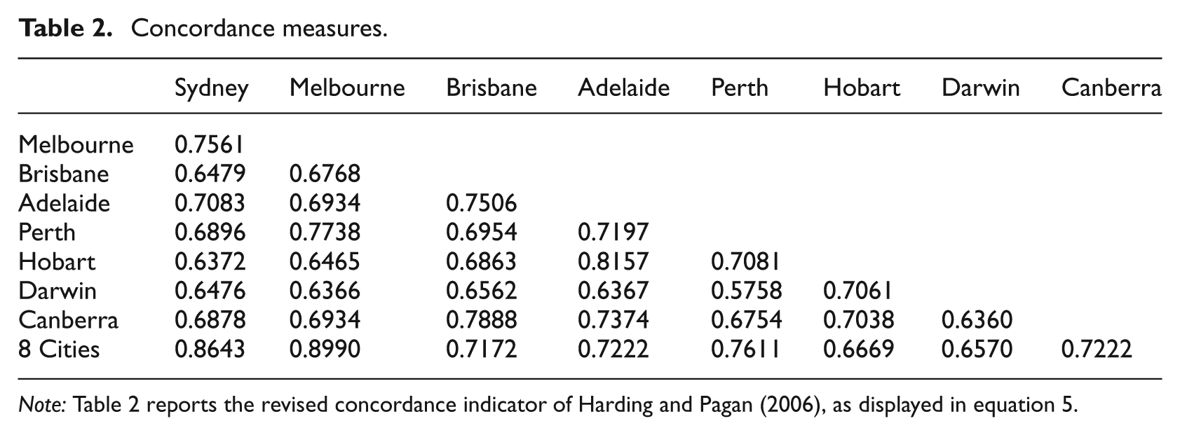
Note: Table 2 reports the revised concordance indicator of Harding and Pagan (2006), as displayed in equation 5.

Table 3.

Rho’s.

	Sydney	Melbourne	Brisbane	Adelaide	Perth	Hobart	Darwin	Canberra
Melbourne	0.3506 (0.0214)
Brisbane	0.0584(0.6237)	0.0649(0.5947)
Adelaide	0.2561(0.0620)	0.1681(0.2151)	0.3246 (0.0027)
Perth	0.1900(0.1602)	0.3667 (0.0006)	0.1467(0.1956)	0.2583 (0.0349)
Hobart	0.0412(0.7042)	−0.0063(0.9446)	0.1070(0.2131)	0.5074 (0.0000)	0.1939(0.1019)
Darwin	0.0800(0.4718)	−0.0183(0.8604)	0.0367(0.7655)	0.0383(0.7305)	−0.1550(0.0799)	0.1883(0.0654)
Canberra	0.2039(0.1122)	0.1681(0.1684)	0.4289 (0.0000)	0.3219 (0.0047)	0.1407(0.2491)	0.2065 (0.0272)	0.0364(0.7445)
8 Cities	0.6429 (0.0000)	0.7078 (0.0000)	0.1818(0.1287)	0.2468(0.1226)	0.3312 (0.0141)	0.0519(0.5929)	0.0390(0.7251)	0.2468(0.0602)

Note: Table 3 reports the rho’s estimated from equation 6. P-values are reported in parentheses. Those estimates that are of significance of at least 5% are displayed in bold.

In contrast, with respect to the remaining centres there are a number of pairings that report significant findings. This is particularly so in the case of Adelaide which is significantly synchronised with Brisbane, Perth, Hobart and Canberra. Three significant pairings are also found with respect to Canberra (Brisbane, Adelaide and Hobart). Both Brisbane and Hobart report two significant rho’s. The main exception is Darwin. If one uses a cut-off of 5% significance then the Darwin market is not significantly synchronised with any other capital city, although marginal levels of significance, below 10%, are noted for Perth and Hobart.

A few issues arise from the analysis. Firstly, it is noticeable that despite the distances involved when examining the Australian market, the importance of contiguous and non-contiguous markets is evident. There is a tendency for markets to be relatively close to each other to be more likely to report evidence of synchronised cycles. One such example can be found for Perth, the most geographically isolated market in Australia, with significant results not reported for the city pairing with Brisbane. Given the finding with Sydney and Melbourne, it is also not that surprising a significant result is also observed with respect to the two smallest centres, Hobart and Darwin, albeit at a marginal level and a p-value of nearly 0.08. In addition, Hobart is significantly related to Canberra. Whilst a larger market than either Darwin or Hobart, Canberra is the smallest mainland city near the east and southern coasts. The majority of the significant findings are between the second tier of cities in terms of population. This can be illustrated also by the fact that the two markets with the highest number of significant results, especially at a 95% level and above, are Adelaide and Canberra. Their economic structure is also of interest in that they are less dependent on sectors such as financial services and the resource sector in comparison to many of the capitals. With respect to the 8 Capital Cities index it is not too surprising that Sydney and Melbourne report significant degrees of concordance given their relative size and weight in the aggregate index. Whilst Canberra is not significantly synchronised with either of its two large neighbours, it is also so with the national index.

One result that warrants further mention is the case of Perth and Darwin. Whilst a significant rho is reported, it is negative in sign. The modified concordance indicator in this case is also the lowest observed (0.5758). These results indicate that these two markets are actually significantly counter cyclical. This could be the result of not only relative spatial isolation from neighbouring markets, but also due to the heavy reliance on a less diverse base for economic growth in those markets when compared to the relatively large and economically diverse regions to the south and east. Most previous studies of house price diffusion and commonalities in the Australian market have not examined Darwin. It is therefore also hard to explicitly compare the findings reported here with those using an alternative methodological framework. The nature of the empirical tests do however have to be considered. It is especially important to remember that the Harding-Pagan framework does not imply anything concerning price diffusion or causality, nor indeed anything concerning the magnitude of the relationship. Rather it considers the degree to which markets spend time in the same phase of a cycle.

Decomposition of housing cycles

The final section of the paper considers the cyclical behaviour of the eight Australian Metropolitan markets in the context of the decomposition approaches of Beveridge and Nelson (1981) and Hodrick and Prescott (1997). Both of these approaches have been used extensively in the economic cycle’s literature to decompose series into their trend and cyclical components. The rationale behind their application in a business cycle context can be easily transferred to a housing market one. By decomposing the series we can isolate the cyclical element that can be defined as being the deviation from the long-term trend. It should be made clear that given the nature of the empirical tests the cyclical and trend components examined do not consider the same features of the respective housing markets as analysed in the preceding empirical analysis on concordance.

The Beveridge-Nelson decomposition separates a time-series (y_t ) into permanent (trend) and transitory (cyclical) components as follows:

y_{t} = P_{t} + T_{t}

(7)

Assuming that y_t is an ARIMA (p,1,q) process we can re-write equation 7 as below:

Δ y_{t} = Δ P_{t} + Δ T_{t}

(8)

Given that the first difference of such a process has a stationary infinite order moving average representation, as displayed in equation 9 below, we can therefore further define Δy_t as in equation 10:

Δ y_{t} = c_{0} e_{t} + c_{1} e_{t - 1} + \dots . = C (L) e_{t}

(9)

Δ y_{t} = C (1) e_{t} + Ψ (L) (1 - L) e_{t}

(10)

where $Ψ (L) = ψ_{0} + ψ_{1} L + \dots .$ is a polynomial with $lim_{j \to \infty} = 0$ . The components can therefore be identified as follows:

Δ P_{t} = C (1) e_{t}

(11)

Δ T_{t} = Ψ (L) (1 - L) e_{t}

(12)

As $Δ T_{t} = (1 - L) T_{t}$ , then $T_{t} = Ψ (L) e_{t}$ . This means that P_t is an I(1) process and T_t is I(0). The Beveridge-Nelson decomposition therefore has two primary characteristics. Firstly, that the shocks in the permanent component are white noise and secondly, that the shocks in the permanent and transitory components are perfectly correlated through the common value (e_t ). To empirically decompose the series in question we therefore estimate the permanent component as follows (Newbold, 1990):

{\bar{y}}_{t} = y_{t} + lim_{k \to \infty} [\sum_{j = 1}^{k} {\hat{w}}_{t} (j)] = y_{t} + c_{t}

(13)

where ${\bar{y}}_{t} = the permanent component of y_{t}$ , ${\hat{w}}_{t} = Δ {\hat{y}}_{t} - μ, μ$ is the mean of the ARIMA $(p, q) process of the permanent component of Δ y_{t}$ , $Δ {\hat{y}}_{t} are the forecasts from a fitted ARMA process of Δ y_{t}$ .

The alternative decomposition model used is that of Hodrick and Prescott (1997). This decomposition is a linear filter that estimates a smoothed trend series. This is achieved by minimising the variance of the original series (y) around the trend (T), subject to a constraint concerning the second difference of T. Therefore, T is selected such that it minimises the following:

\sum_{t = 1}^{T} {(y_{t} - T_{t})}^{2} + λ \sum_{t = 2}^{T - 1} {[(T_{t + 1} - T_{t}) - (T_{t} - T_{t - 1})]}^{2}

(14)

The parameter λ controls for the smoothness of the series. For the purposes of this paper we use the frequency power rule of Ravn and Uhlig (2002). This is defined such that the number of periods per annum is divided by 4, squared and multiplied by 1600. Given that we have quarterly data this provides a figure of 1600 for our purposes.

The results from the two decompositions are displayed in Figures 2 and 3 and Table 4. Figure 2 displays the trends estimated from the two approaches, whilst the corresponding cyclical estimates are displayed in Figure 3. As would be expected the Hodrick-Prescott Filter provides smoother trends than the corresponding Beveridge-Nelson estimates, as can be clearly seen in Figure 2. This also means that a higher proportion of the variability of the series is captured in the cyclical element of the Hodrick-Prescott decomposition. Therefore, the cyclical elements may display greater variation, a feature that is also captured in the standard deviation figures reported in Table 4 in the case of four of the eight markets. The reason behind this difference is that the Beveridge-Nelson decomposition defines the trend as the random walk component. It would therefore be expected that it capture more variability in comparison to the Hodrick-Prescott approach. Table 4 reports the correlations between the cyclical elements for each of the eight markets, together with the standard deviation and the first order autocorrelation of the cyclical elements. The results illustrate a degree of divergence across the cities in terms of the correlations across the cyclical components. Indeed, the correlations are in many respects supportive of the results from the concordance indicators.

Figure 2.

Beveridge-Nelson and Hodrick-Prescott trends.

Figure 3.

Beveridge-Nelson and Hodrick-Prescott cycles.

Table 4.

Correlation matrix and standard deviations for cyclical components.

	Sydney	Melbourne	Brisbane	Adelaide	Perth	Hobart	Darwin	Canberra	StDev	ρ
Panel A: Beveridge-Nelson cycles
Sydney	1.0000								4.3292%	0.5335
Melbourne	0.5789	1.0000							1.8332%	0.3491
Brisbane	0.3857	0.3368	1.0000						6.6897%	0.7035
Adelaide	0.2047	0.2137	0.6640	1.0000					3.5183%	0.7607
Perth	0.3812	0.3840	0.3147	0.1166	1.0000				5.2818%	0.5928
Hobart	0.1886	0.1979	0.6666	0.6454	0.3361	1.0000			6.4278%	0.7565
Darwin	−0.2698	−0.1033	0.0341	0.0841	0.1693	0.3076	1.0000		5.0182%	0.8477
Canberra	0.5569	0.5021	0.6990	0.4913	0.4111	0.5422	−0.0757	1.0000	3.6877%	0.6205
Panel B: Hodrick-Prescott cycles
Sydney	1.0000								5.7602%	0.9067
Melbourne	0.8165	1.0000							4.8484%	0.8365
Brisbane	0.5185	0.3867	1.0000						5.0775%	0.9079
Adelaide	0.4702	0.4125	0.8503	1.0000					3.4841%	0.8221
Perth	0.3547	0.4179	0.1000	−0.0385	1.0000				6.2270%	0.9180
Hobart	0.2715	0.0423	0.7006	0.5639	0.1839	1.0000			5.2038%	0.9055
Darwin	−0.2702	−0.3098	0.0426	−0.0400	0.3284	0.3696	1.0000		3.7771%	0.8320
Canberra	0.5649	0.3747	0.7877	0.6954	0.0218	0.5139	−0.0467	1.0000	4.7168%	0.9001

Note: This table reports summary data based upon the cyclical series’ estimated for each of the eight metropolitan housing markets. Correlations are estimated for each pairing of the cyclical components. The final two columns report the standard deviation of the cyclical components and the first order autocorrelation of each series (ρ) respectively.

As with the previous results the strong relationship between the two largest metropolitan areas, Sydney and Melbourne, is evident. In the case of the Beveridge-Nelson decomposition the cyclical elements for the two markets have a correlation of 0.5789, the highest coefficient reported for either city. The corresponding coefficient when using the Hodrick-Prescott framework is 0.8165, and again the highest noted for either Sydney or Melbourne. Indeed, with the exception of Canberra, the only case where either Sydney or Melbourne report a correlation above 0.50 is with Brisbane in the case of Sydney with the Hodrick-Prescott decomposition.

A key finding earlier in the concordance analysis was that strong relationships were observed amongst the smaller markets, especially those in the east of Australia, a result that is echoed in these tests. Correlations in excess of 0.50 are observed for the pairings of Adelaide–Brisbane, Brisbane–Hobart, Brisbane–Canberra, Adelaide–Hobart and Canberra–Hobart in the case of the Beveridge-Nelson results. Only the two most isolated centres, Perth and Darwin, see no correlation in excess of 0.50 with any other market using either decomposition technique. While consistent with the concordance analysis, the results for Perth and Darwin suggest that their reliance on mining and resources for economic growth over the time period further separates their house price movements not only just from the more urban areas of the country, but also other relatively less isolated markets in Australia that are reliant on agriculture and other economic sectors for growth. In addition, whilst the majority of the correlations are significant at a 5% level, the exceptions are predominantly found with respect to Darwin or Perth. For Darwin, the correlations with Adelaide, Brisbane and Canberra are not significant with both decomposition techniques, whilst for Perth the coefficients with respect to Adelaide and Canberra aren’t significant with the Beveridge-Nelson data.¹¹

The results with respect to the correlations do not however reveal parallels in the standard deviations reported. There are also quite distinct differences in the volatility of the cyclical components in either framework. In the Beveridge-Nelson case the market with the highest volatility is Brisbane, whilst with the Hodrick-Prescott data, this is the case with Perth. Broadly speaking the cyclical component tends to be highest across the two methodologies, in Sydney, Hobart and the aforementioned Brisbane and Perth. These four cut across the three broad groupings of Sydney–Melbourne, the remaining eastern cities and the outlying Perth and Hobart. The differences observed in the volatilities are consistent with previous work on business cycles, such as Carlino and Sill (2001) in their analysis of regional income cycles in the US.

Concluding comments

The analysis of interlinkages across metropolitan housing markets has largely considered the issue from the perspective of house price diffusion and convergence. This study has examined the commonalities present in the cyclical behaviour of eight metropolitan centres in Australia using approaches originated in the business cycle literature. Both the measure of concordance of cycles and the decomposition of the price series into their permanent and cyclical elements provide complementary evidence to the existing Australian empirical literature. Sydney and Melbourne, as the two largest markets, display a high degree of interaction and commonalities using either approach. However, in the vast majority of cases these commonalities are not extended to the remaining six markets. In contrast however, there is widespread evidence of synchronisation using either empirical approach, with the remaining markets, and in particular those markets on the eastern and southern seaboards of Australia.

While this empirical framework provides additional support to the notion that Sydney and Melbourne have distinct cyclical features in relation to the remaining metropolitan markets, the decomposition of the cyclical components suggests areas for further research on the role that demand for resources, and in particular the export of resources, might mean for understanding the relationships between house prices in these cities. Given the relative isolation of many Australian cities and less economic diversification of smaller urban centres, additional research is suggested on the roles that demand for resources and economic growth from countries outside of Australia may play on these housing markets. The results are consistent with much of the existing work to have considered Australia, and given the different empirical framework adopted, provides additional support to the notion that Sydney and Melbourne have distinct cyclical features in comparison to the remaining metropolitan centres in Australia.

The paper does only consider specific aspects of the relationships between the eight capital cities. The methodological framework adopted doesn’t consider either non-contemporaneous features in the shape of either house price diffusion or the response to common shocks. However, the results do highlight a number of issues in terms of the commonalities in cyclical behaviour that may be explored in greater depth in the context of house price diffusion.

Footnotes

Funding

This research received no specific grant from any funding agency in the public, commercial, or not-for-profit sectors.

Notes

References

Alexander

Barrow

(1994) Seasonality and cointegration of regional house prices in the UK. Urban Studies 31: 1667–1689.

Allen

Amano

Byrne

. (2009) Canadian city housing prices and urban market segmentation. Canadian Journal of Economics 42: 1132–1149.

Altavilla

(2004) Do EMU members share the same business cycle. Journal of Common Market Studies 42: 869–896.

Ashworth

Parker

(1997) Modelling regional house prices in the UK. Scottish Journal of Political Economy 44: 225–246.

Australian Bureau of Statistics (2011) 5220.0 − Australian national accounts: State accounts, 2010–11. Available at: http://www.abs.gov.au/AUSSTATS/abs@.nsf/DetailsPage/5220.02010–11?OpenDocument.

Australian Bureau of Statistics (2012) 3101.0 − Australian demographic statistics, June 2012. Available at: http://www.abs.gov.au/AUSSTATS/abs@.nsf/allprimarymainfeatures/33970B13F1DF7F56CA257B3B00117AA2?opendocument.

Beveridge

Nelson

(1981) A new approach to decomposition of economic time series into permanent and transitory components with particular attention to measurement of business cycle. Journal of Monetary Economics 7: 151–174.

Bilgin

Lau

CKM

Demir

. (2010) Rental price convergence in a developing economy: New evidence from nonlinear panel unit root test. International Journal of Strategic Property Management 14: 245–257.

Bourassa

Hendershott

(1995) Australian capital city real house prices, 1979–1993. The Australian Economic Review 111: 16–26.

10.

Carlino

Sill

(2001) Regional income fluctuations: Common trends and common cycles. The Review of Economics and Statistics 83: 446–456.

11.

Chien

M-S

(2010) Structural breaks and the convergence of regional house prices. Journal of Real Estate Finance and Economics 40: 77–88.

12.

Clapp

Tirtiroglu

(1994) Positive feedback trading and diffusion of asset price changes: Evidence from housing transactions. Journal of Economic Behavior & Organization 24: 337–355.

13.

Clark

Coggin

(2009) Trends, cycles and convergence in US regional house prices. Journal of Real Estate Finance and Economics 39: 264–283.

14.

Cook

(2003) The convergence of regional house prices in the UK. Urban Studies 40: 2285–2294.

15.

Cook

(2005a) Detecting long-run relationships in regional house prices in the UK. International Review of Applied Economics 19: 107–118.

16.

Cook

(2005b) Regional house price behaviour in the UK: Application of a joint testing procedure. Physica A 345: 611–621.

17.

Cook

(2006) A disaggregated analysis of asymmetrical behaviour in the UK housing market. Urban Studies 43: 2067–2074.

18.

Costello

Fraser

Groenewold

(2011) House prices, non-fundamental components and interstate spillovers: The Australian experience. Journal of Banking & Finance 35: 653–669.

19.

Del Negro

Otrok

(2007) 99 Luftballons: Monetary policy and the house price boom across US states. Journal of Monetary Policy 45: 1962–1985.

20.

Drake

(1995) Testing for convergence between UK regional house prices. Regional Studies 29: 357–366.

21.

Dvornak

Kohler

(2007) Housing wealth, stock market wealth and consumption: A panel analysis for Australia. Economic Record 83: 117–130.

22.

Elliot

Rosenberg

Stock

(1996) Efficient tests for an autoregressive unit root. Econometrica 64: 813–836.

23.

Fadiga

Wang

(2009) A multivariate unobserved component analysis of US housing market. Journal of Real Estate Finance and Economics 40: 77–88.

24.

Fratantoni

Schuh

(2003) Monetary policy, housing and heterogeneous regional markets. Journal of Money, Credit and Banking 35: 557–589.

25.

Fry

Martin

Voukelatos

(2010) Overvaluation in Australian housing and equity markets: Wealth effects or monetary policy. Economic Record 86: 465–485.

26.

Giussani

Hadjimatheou

(1991) Modelling regional house prices in the United Kingdom. Papers in Regional Science 70: 201–219.

27.

Gupta

Miller

(2012) The time-series properties of house prices: A case study of the Southern California market. Journal of Real Estate Finance and Economics 44: 339–361.

28.

Harding

Pagan

(2001) Some Econometric Problems with Regressions using Constructed State Variables. Mimeo.

29.

Harding

Pagan

(2002) Dissecting the cycle: A methodological investigation. Journal of Monetary Economics 49: 365–381.

30.

Harding

Pagan

(2006) Synchonization of cycles. Journal of Econometrics 132: 59–79.

31.

Hatzvi

Otto

(2008) Prices, rents and rational speculative bubbles in the Sydney housing market. Economic Record 84: 405–420.

32.

Hodrick

Prescott

(1997) Postwar US business cycles: An empirical investigation. Journal of Money, Credit and Banking 29: 1–16.

33.

Holly

Jones

(1997) House prices since the 1940s: Cointegration, demography and asymmetries. Economic Modelling 14: 549–565.

34.

Holly

Pesaran

Yamagata

(2010) A spatio-temporal model of house prices in the USA. Journal of Econometrics 158: 160–173.

35.

Holly

Pesaran

Yamagata

(2011) The spatial and temporal diffusion of house prices in the UK. Journal of Urban Economics 69: 2–23.

36.

Holmes

(2007) How convergent are regional house prices in the United Kingdom? Some new evidence from panel data unit root testing. Journal of Economic and Social Research 9: 1–17.

37.

Holmes

Grimes

(2008) Is there long-run convergence among regional house prices in the UK? Urban Studies 45: 1531–1544.

38.

Holmes

Otero

Panagiotidis

(2011) Investigating regional house price convergence in the United States: Evidence from a pair-wise approach. Economic Modelling 28: 2369–2376.

39.

Jackson

Stevenson

Watkins

(2008) NY-LON: Does a single cross-continental office market exist? Journal of Real Estate Portfolio Management 14: 79–92.

40.

Kuethe

Pede

(2011) Regional housing price cycles: A spatio-temporal analysis using US state level data. Regional Studies 45: 563–574.

41.

Lee

Reed

(2011) Volatility decomposition of Australian housing prices. In: PRRES 2011: Proceedings of the 17th Pacific Rim Real Estate Society annual conference, Pacific Rim Real Estate Society, Gold Coast, Qld, Australia, 16–19 January 2011.

42.

Luo

Liu

Picken

(2007) Housing price diffusion pattern of Australia’s state capital cities. International Journal of Strategic Property Management 11: 227–242.

43.

Liu

(2010) The decomposition of housing market variations: A panel data approach. International Journal of Housing Market and Analysis 3: 6–16.

44.

MacDonald

Taylor

(1993) Regional house prices in Britain: Long-run relationships and short-run dynamics. Scottish Journal of Political Economy 40: 43–55.

45.

Meen

(1999) Regional house prices and the ripple effect: A new interpretation. Housing Studies 14: 733–753.

46.

Meen

Andrew

(1998) Modelling regional house prices: A review of the literature. Report, Department of the Environment, Transport and the Regions.

47.

Muellbauer

Murphy

(1994) Explaining regional house prices in the UK. Working paper, Department of Economics, University College Dublin, Ireland, November.

48.

Munro

(1996) UK house price dynamics: Past and future trends. Research report, Council of Mortgage Lenders, London, UK.

49.

Newbold

(1990) Precise and efficient computation of the Beveridge-Nelson decomposition of economic time series. Journal of Monetary Economics 26: 453–457.

50.

Oikarinen

(2006) The diffusion of housing price movements from center to surrounding areas. Journal of Housing Research 15: 3–28.

51.

Pollakowski

Ray

(1997) Housing price diffusion patterns at different aggregation levels: An examination of housing market efficiency. Journal of Housing Research 8: 107–124.

52.

Ravn

Uhlig

(2002) On adjusting the Hodrick-Prescott filter for the frequency of observations. The Review of Economics and Statistics 84: 371–375.

53.

Riddel

(2011) Are housing bubbles contagious? A case study of Las Vegas and Los Angeles home prices. Land Economics 87: 126–144.

54.

Sanjuan

Dawson

Hubbard

. (2009) Rents and land prices in Japan: A panel cointegration approach. Land Economics 85: 587–597.

55.

Stevenson

(2004) House price diffusion and inter-regional and cross-border house price dynamics. Journal of Property Research 21: 301–320.

56.

(2000) Segmentation of Australian housing markets: 1989–98. Journal of Property Research 17: 311–327.

57.

Yates

(2002) Housing implications of social, spatial and structural change. Housing Studies 17: 581–618.