




Abstract
The structure of transportation networks and the patterns of accessibility they give rise to are an important determinant of land prices, and hence urban spatial structure. While there is ample evidence on the cross-sectional relationship between location and land value (usually measured from the value of improved property), there is much less evidence available on the changes in this relationship over time, especially where location is represented using a disaggregate measure of urban accessibility. This paper provides evidence of this dynamic relationship using data on home sales in the Minneapolis-St Paul, MN, USA metropolitan area, coupled with disaggregate measures of urban accessibility for multiple modes, for the period from 2000 to 2005. Our investigation tracks the effects of marginal changes in accessibility over time, as opposed to static, cross-sectional relationships, by using an approach in which the unit of observation is a ‘representative house’ for each transportation analysis zone in the region. This approach allows us to control for changes in structural attributes of houses over time, while also isolating the effect of changes in accessibility levels. Results of this approach are compared with a cross-sectional model using the same variables for a single year to illustrate important differences. Empirical estimates indicate that while most of the models estimated using a cross-sectional specification yield positive and significant effects of accessibility on sale prices, these effects disappear when the models are transformed into first-difference form. We explain these findings in light of the state of maturity of urban transportation networks.
Introduction
While much is known about the relationship between transportation networks, accessibility and land values, most of the accumulated evidence to date has been drawn from cross-sectional or pooled cross-section/time series analyses that represent the relationship between location and land value at a single point in time. Typically the unit of analysis is property transactions within an urban area or some subset of it. While this approach may provide an estimate of the relationship between location and land value across locations within an urban area at some point in time, the estimate is often heavily influenced by observations located in areas that are already developed and may already have relatively high levels of accessibility. The estimated relationship is typically assumed to be linear or perhaps linear in the logarithms of the variables, and thus predicts a relatively stable relationship across space (and time, if that dimension is included). The implicit assumption is that new projects that result in accessibility changes will have impacts on land values that roughly follow these previously estimated relationships. These models may not be as useful for predicting the impacts of large and/or abrupt changes in accessibility resulting from major transportation improvements in locations that do not already enjoy high accessibility. Likewise, they may overpredict the impacts of projects in established locations, where transportation networks are relatively complete and patterns of accessibility are unlikely to change greatly.
This paper examines the dynamic relationship between accessibility (defined as the ease of reaching desired destinations, such as employment) and land value over time, and asks whether changes in levels of accessibility over time and across locations can predict changes in land value (measured here using house prices) with the same consistency that most cross-sectional analyses do. To do so, we use property sales data from the Minneapolis-St Paul, Minnesota (USA) region for the years 2000 and 2005, along with disaggregate measures of accessibility to jobs for multiple modes, to estimate models which predict changes in prices over time in a particular location. Our method, which we term a ‘representative house’ approach, uses the transportation analysis zone (TAZ) as a unit of analysis, rather than individual housing units. It attempts to combine the use of statistical controls for important structural attributes of a property that are common in hedonic price function studies with the ability to observe changes in prices at a particular location over time, thus giving estimates of the impact of marginal changes in accessibility. This method will be discussed more fully later in the paper.
The paper is structured as follows. The next section provides a short overview of the history of empirical approaches to the study of location and land value. The following section introduces our empirical approach and the data sets used in the analysis. Then, results are presented and compared for models that use static, cross-sectional and first differences specifications. The comparison of these models is then used to inform a discussion of the practical and methodological issues associated with studies of location, accessibility and land values. The paper concludes with some prospective ideas about improving our understanding of this relationship.
Background
Urban researchers have long recognised the relationship between location and land value. During the 1960s, urban economists began to develop formal theoretical frameworks which predicted land value as a function of location relative to a single central business district (CBD) (Alonso, 1964; Mills, 1967). These monocentric models gained widespread acceptability because of their ability to both analytically describe the tradeoffs between location and housing or land consumption and also to offer a framework for empirically investigating elements of the theory (Mills, 1969). The concept of accessibility was embodied in the variable measuring distance from the CBD.
While the original monocentric model made simplifying assumptions about transportation, namely that it was ubiquitous and available via a single mode, the urban economic literature has seen subsequent extensions to account for multiple modes (Anas and Moses, 1979; LeRoy and Sonstelie, 1983) and non-ubiquitous availability, as in the case of fixed-route streetcar lines (Steen, 1986). Voith (1991) adopted a measure of public transit accessibility for Philadelphia’s rail networks based on service quality and travel time to the CBD, which was then used to examine its influence on house prices in the region.
Variations on the theme of the monocentric model became standard for empirical studies of land values during the 1970s and 1980s. A wide variety of studies were able to replicate evidence of a rent gradient that declined with distance from the CBDs of cities in many developed countries. However, many analysts noted the increasingly polycentric nature of urban areas, especially in the USA, where decentralisation of both households and employment occurred most rapidly. The development of urban subcentres provided a challenge to the monocentric model (Gordon et al., 1986; McDonald, 1987; Redfearn, 2007; Richardson, 1988) and necessitated modifications to empirical specifications of models predicting land prices, often involving incorporation of additional variables measuring distances to multiple employment centres (Heikkila et al., 1989; McDonald and McMillen, 1990; Richardson et al., 1990; Waddell et al., 1993).
Representation of urban space at more disaggregate levels has been more common in fields such as geography, urban planning and transportation engineering, where the need to develop practical models (with fewer theoretical constraints) for forecasting urban traffic flows led naturally to the use of disaggregate data sets containing data on the location of households and urban activities at a small level of geography. These data lent themselves easily to development of measures of accessibility, tying together the characteristics of transportation networks with the locations of the activities they serve (Hansen, 1959; Wachs and Kumagai, 1973), and providing a superior measure of location in increasingly decentralised urban areas.
Evidence of the use of disaggregate measures of urban accessibility can be found in some older empirical studies of the determinants of the value of urban land and housing. Brigham (1965) used a measure of ‘accessibility potential’ to employment in a study of land values in Los Angeles which closely resembles the zone-based measures of accessibility associated with gravity-type models of spatial interaction. Another study by Nelson (1977) recognised the importance of more flexible measures of accessibility, testing six of them, including a cumulative opportunity-type measure of employment, in hedonic price regressions for residential properties in Washington, DC. The results of the regressions, fitted to 1970 data, were used to infer the value of time spent in commuting. For the most part however, studies of the value of location which employ disaggregate accessibility measures have been a more recent phenomenon. Examples, drawn mostly from the transportation and urban planning literature, include Srour et al. (2002), Franklin and Waddell (2003), Mathur (2008) and Martinez and Viegas (2009).
Another aspect of studies of the value of urban location that is comparatively underrepresented is the evaluation of changes in land prices in response to changes in the relative accessibility of a location over time. Some studies have used historical data over relatively long time periods to examine changes in the urban rent gradient (Atack and Margo, 1998; Edel and Sclar, 1975; McMillen, 1996; Wheaton et al., 2009). However, most these studies employ some form of the monocentric model as a strategy to deal with limited data, and thus are restricted to a relatively simple treatment of space. The fitted models also tend to take the form of repeated cross-sectional estimates at different points in time. One exception is a recent paper by Gibbons and Machin (2005) which observes differences in house prices over a shorter period (four years) resulting from an extension of the London rail network. However, the treatment of accessibility is again restricted to CBD distance and distance to the nearest rail station. The present paper offers an alternative approach based on observed changes in both urban accessibility and house prices in order to estimate the response of location premia to changes in urban structure over time.
Methodology
Ideally, one would like to be able to observe the same housing unit in the same location over time, holding housing attributes constant and thus restricting the sources of change in the attractiveness of a house to external effects such as changes in its relative accessibility within an urban area. Repeat sales methods represent one option for doing this and have in fact been used in a couple of instances to estimate the impacts of new transportation projects (Archer et al., 1996; Gatzlaff and Smith, 1993). In the current context however, they would be difficult to implement. The need to disaggregate space into something that can be measured as a continuous rather than discrete variable (using zone-level accessibility), and the limited temporal availability of our accessibility data, imply that a method must be chosen which is capable of using all available data on sales at given points in time.
We refer to our method as the ‘representative house’ approach. The representative house is essentially a statistical construct that captures the features of all houses sold within a particular location, in this case a TAZ, at some point time. Owing to the strong possibility that house prices and several salient housing and property attributes may be non-normally distributed, we use median values to capture the features of the representative house in each zone at each point in time. Thus, any observed changes in the median sale price of the representative house in a particular zone over some period of time are assumed to be a function of changes in the attributes of the representative house (e.g. age, square footage, lot size) along with changes in its accessibility, measured here as accessibility to jobs within a specified time threshold. While the authors are unaware of any other studies that have used the exact same approach to study this topic, a similar type of method was used by McMillen (2008) to decompose changes in the house price distribution over time into changes in structural characteristics, neighbourhood factors and changes in coefficient values using quantile regression. This method differed from the one presently employed in that it attempted to evaluate changes in house prices over time as a function of both changes in housing attributes and changes in the distribution of the coefficients, implying changes in the values placed on certain housing attributes. Also, the use of quantile regression allowed the regression coefficients to vary across the distribution of house prices, allowing for heterogeneous effects of certain attributes at different price levels.
The empirical model that is used to operationalise the relationship between changes in accessibility and house prices is specified in first-difference form, such that the dependent and independent variables measure changes in the value of these variables between 2000 and 2005. Formally, the model may be written as:

where ΔPi represents the change in the median sale price for houses in zone i between 2000 and 2005, ΔAGEi is the change in the median age of houses that sold in zone i between 2000 and 2005, ΔSQFTi is the change in the median square footage of houses that sold in zone i between 2005 and 2005, ΔACCESSi denotes the change in accessibility to jobs in zone i between 2000 and 2005, α 1 through α 4 are parameters to be estimated, and ei is a disturbance term with zero mean and constant variance. Accessibility in this study is measured in terms of jobs accessible within 20 minutes, with this threshold established by zone-to-zone travel times. The basic specification will consider only accessibility by auto, though access by other modes (public transit and walking) will be tested as well.
Data
In order to estimate the models just described, it is necessary to have data on both regional accessibility and home sales at two points in time, at a minimum. The accessibility data used in this study are the product of a pair of previous studies (Krizek et al., 2009; Levinson et al., 2010) and are available in five-year increments between 1995 and 2005. We use the years 2000 and 2005 to illustrate our method, owing to the limited availability of home sales data in an appropriate, digital format for several years prior to 2000. Construction of the sample of home sales data required the use of three different data sources to ensure a high enough degree of completeness for the analysis that follows. These three sources were:
Home sales data from the Minnesota Department of Revenue for the years 2000 and 2005.
Parcel-level property records assembled by the Metropolitan Council of the Twin Cities using data reported from the seven counties over which it has jurisdiction.
Home sales data from the Multiple Listing Service (MLS), a local real estate data management firm, for the years 2001 and 2004.
The home sales data from the Department of Revenue form the backbone of the data set used for the analysis. While this data source contains sales data on a variety of property types, we focus on sales of residential units. This excludes multifamily rental apartments from the data set, but it does include condominiums and townhomes. Since these data are not inherently spatial, they needed to be joined to the Metropolitan Council’s parcel files. Doing so accomplished two important objectives. First, they permitted the home sales data to be mapped and spatially linked to the accessibility data, which were available at Census block and TAZ levels. Second, the parcel files were an important source of data on housing and parcel attributes which serve as statistical controls for the models that relate accessibility to house prices.
One major weakness of the parcel files is that they are reported by individual counties, which tend to vary considerably in terms of the attribute information they report. Our empirical analysis of zone-level prices and price changes includes three major housing and parcel attributes as controls: lot (parcel) size, house square footage and age of house.
Since the three attributes of interest were not universally available, some adjustments had to be made to provide a relatively complete data set. The core seven counties of the region account for about 2.8 million people spread across 1200 TAZs. Ideally, all 1200 TAZs would be used as the basis for the empirical analysis of accessibility change. As a practical matter, two counties were removed from the analysis. Scott County contained none of the attributes needed for the analysis. Given its relatively small population size, it was summarily dropped from the analysis. Washington County, on the eastern edge of the region, was also removed from consideration. Despite the completeness of the attribute data for this county, the home sales data from the Department of Revenue could not be matched to the parcel files, and so could not be displayed spatially. The locations of each of the counties in the region, including those removed from the data set, are indicated in Figure 1.
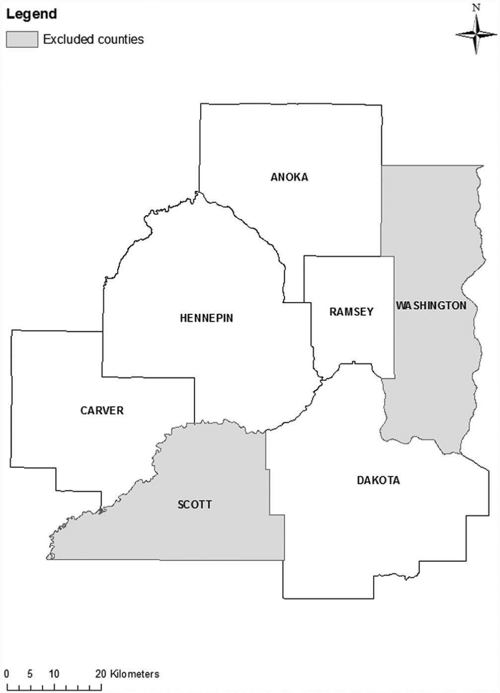
Metropolitan counties excluded from the data set.
For the remaining counties, where instances of missing data arose, the attributes were retrieved from MLS sales data for these counties during the years 2001 and 2004, these being the years that most closely matched the time period used in our study (2000 and 2005). In the case of Hennepin County, the region’s most populous county, data on median square footage of houses sold during 2001 and 2004 were used to substitute for the corresponding missing records in the parcel files for this county in 2000 and 2005.
Considering that two of the seven counties were removed from the analysis, the final number of TAZs which could be used as observations was significantly smaller than the original 1200. Another factor which reduced the final number of TAZs that could be analysed was the requirement that a TAZ had to have a valid sale in each of the two years in order to be considered. The final number of TAZs that met these criteria and were deemed suitable for further analysis was 860. Among the five counties for which home sales were included, there were over 34,000 total sales transactions in 2000 and over 41,000 in 2005.
Figure 2 displays histograms of the number of observed sales for each TAZ in each of the two years. For the year 2000 data, the number of sales varies from a minimum of 1 to a maximum of 220, with a mean of 30. Seventy-two percent of zones contain at least ten sales, while 86% contain at least five. In contrast, the 2005 data have an average of 42 sales per TAZ, with a minimum of 1 and a maximum of 342 sales. Seventy-nine percent of zones contain at least ten sales, while 88% of zones contain at least five.
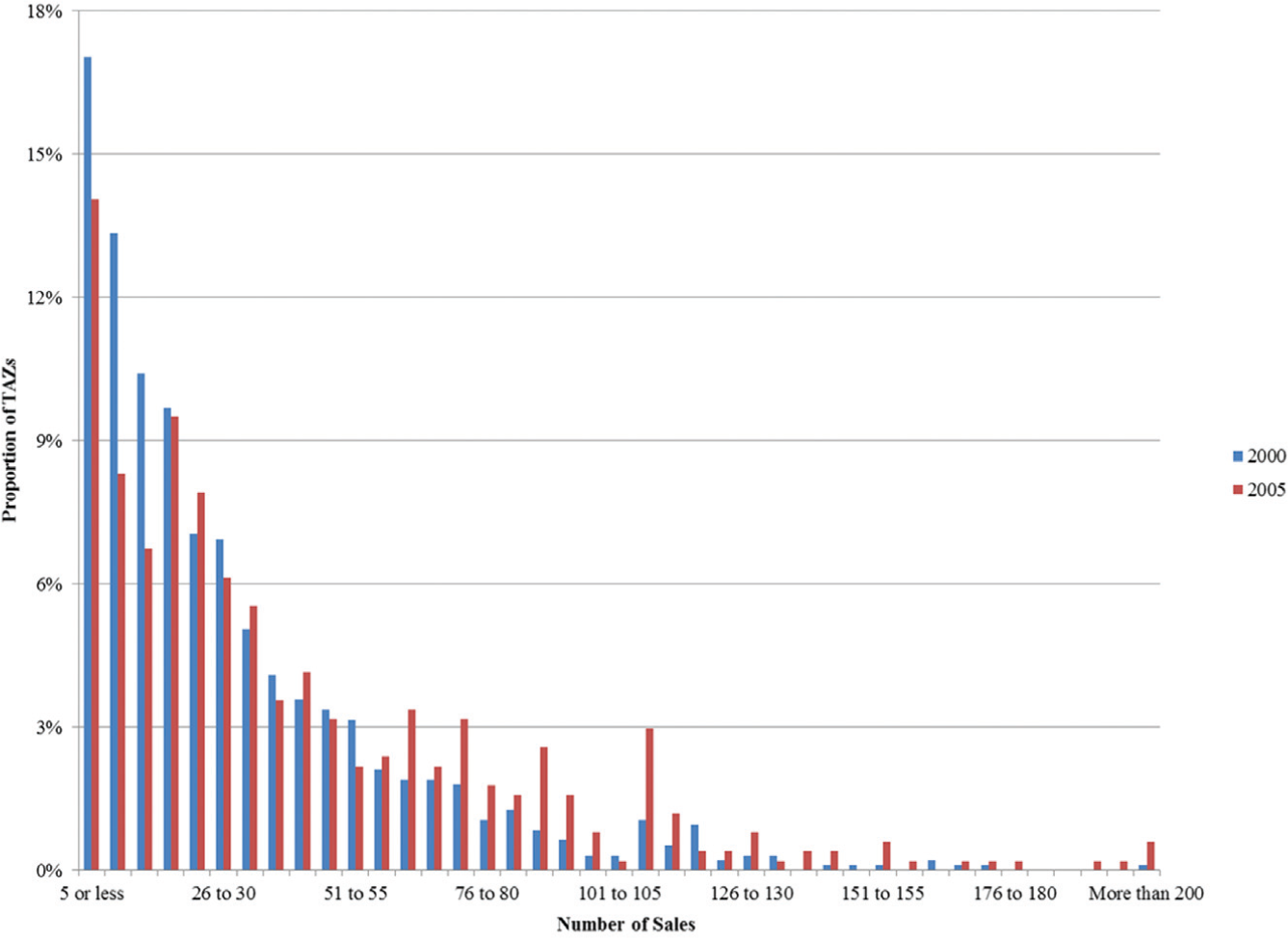
Histogram for proportion of TAZs containing a given number of observed sales, 2000 and 2005.
Each of the sales transactions were joined to regional accessibility data for their respective years. A sample of these data showing access to employment region-wide in 2000 and 2005 is displayed in Figure 3. Accessibility via three separate modes (walking, public transit and car) was considered using cumulative opportunity measures which calculate travel time thresholds based on travel times between zone centroids. The calculation of accessibility by walking was conducted at the Census block level, a lower level of aggregation than TAZs, as this scale was considered more appropriate to the characteristics of the mode. The primary focus was on access to employment, since this measure was the most consistently available across the different modes during both years. A measure of access to workers by car was also included, along with access to employment within different travel time thresholds to examine the sensitivity of the valuation of access to the demarcation of different travel sheds.
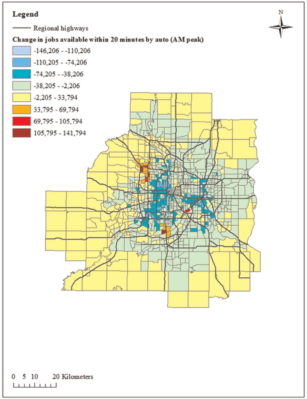
Change in accessibility to employment by car within 20 minutes in the Minneapolis-St. Paul region, 2000 to 2005.
Analysis
A central hypothesis of this study is that the marginal impact of changes in accessibility over time will differ from those obtained using a cross-sectional sample. To facilitate the comparison, we present the results of our representative house model using both cross-sectional data from 2000 and data in first-difference form reflecting changes in prices, housing attributes and accessibility over time. Table 1 presents a list of the variables included in the analysis, along with their descriptions.
Variable names and descriptions.
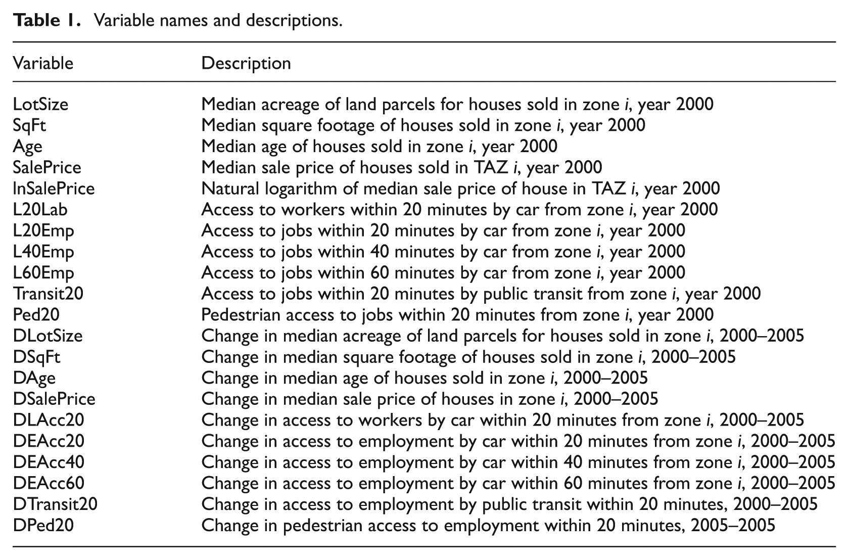
As Table 1 describes, the variables considered for the analysis include basic housing and property attributes, along with several accessibility variables covering different modes and travel sheds. These variables were chosen because they can be measured on a continuous scale, can vary over time and, taken together, represent some of the most important determinants of house prices. Descriptive statistics for both the cross-section variables and the differenced variables measuring 5-year changes are listed in Table 2.
Descriptive statistics for home sales and accessibility data.

Cross-sectional analysis
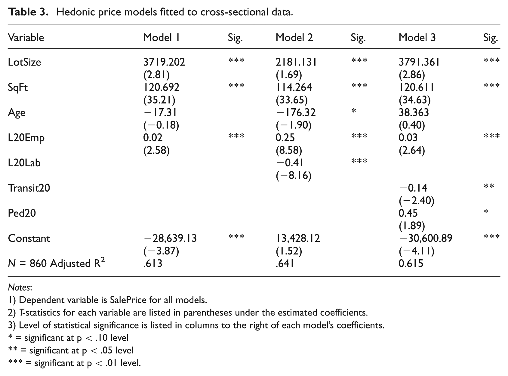
As a point of comparison, and to demonstrate the validity of the representative house approach, we first estimate the model using cross-sectional data from 2000. The basic specification includes the attribute variables representing the median age, square footage and lot size of houses selling in each TAZ during the year 2000, along with a measure of employment accessible by car within a 20-minute travel time threshold. This model is labelled ‘Model 1’ in Table 3 below, and is estimated in linear form.
Hedonic price models fitted to cross-sectional data.
Notes:
1) Dependent variable is SalePrice for all models.
2) T-statistics for each variable are listed in parentheses under the estimated coefficients.
3) Level of statistical significance is listed in columns to the right of each model’s coefficients.
= significant at p < .10 level
= significant at p < .05 level
= significant at p < .01 level.
Each of the other three models summarised in Table 3 represents a variation on the basic specification of Model 1. Model 2 adds a measure of access to workers (labour accessibility) from each zone to the basic specification. Model 3 adds measures of employment access by public transit and walking to the initial measure of access by car. The results reported in Table 3 indicate that even with a relatively limited specification, the models account for more than 60% of the variance in median sale prices across zones. Moreover, the fit of the model does not vary greatly across different specifications.
Given that the functional form of Model 1 is linear, we can interpret the coefficient on the employment accessibility variable as indicating that, all else constant, each additional 100,000 jobs available within a 20-minute drive is associated with a US$2,000 increase in the sale price of a house. Interestingly, the magnitude of this coefficient (though not the sign) increases dramatically when a labour accessibility variable is added to the model. The coefficient on the labour access variable has the expected sign (negative), and its magnitude is even larger than that of the employment access variable. Of note, however, the employment and labour access variables in Model 3 are highly correlated (r = 0.97), and a set of variance inflation factors computed for the regressors in this model indicate rather high values for each of the accessibility variables, over 22 and 21, respectively, which may be indicative of collinearity. Hence, their coefficients should be interpreted with some caution.
In Model 3, variables measuring employment access by walking and public transit are included, along with the standard employment access by car variable. The coefficients on the transit and walking access variables have opposing signs, and both have rather large magnitudes relative to the variable measuring access to employment by car. Again, it should be noted that both the walking and transit access variables are fairly strongly correlated with the car access variable (r = 0.40 and 0.57, respectively), as well as with each other, making it difficult to determine the unique contribution of each of the modal access variables to house prices.
In addition to mode-specific accessibility and measures which differentiate between employment and workers, we also tested travel time thresholds of 40 and 60 minutes rather than 20, in the measurement of employment accessibility by car. At these higher thresholds the marginal effect of an additional job was found to be smaller and statistically insignificant in both cases. This smaller effect may be due to the fact that one can typically reach a considerably larger number of jobs within 40 or 60 minutes than in 20, as can be confirmed by looking at Table 2. It may be true that the extra jobs that are available at these greater distances are not as highly valued by consumers searching among competing locations. This is corroborated by recent (2005–2009) commuting data for the Minneapolis-St Paul region from the American Community Survey (ACS), which suggest that commutes of these durations are fairly rare within the region. Only 13.6% of workers who did not work at home reported having commutes longer than 45 minutes. The corresponding figure for commutes exceeding 60 minutes was 5.7%.
Analysis of price changes
The representative house models fitted to cross-sectional data seem to predict house prices by location fairly well, even with relatively few explanatory variables. We now test the ability of the same modelling approach to predict changes in the median sale price of houses by zone between 2000 and 2005. All of the variables used in this part of the analysis are the differenced variables referred to in the lower halves of Tables 1 and 2. Similar to the cross-sectional analysis, all of the models in this part of the analysis will use a linear specification. This is primarily due to the limitation of using differenced variables. Since a log-linear model would imply a logged dependent variable, it would be impossible to define this variable in cases where the median sale price of houses in any zone declined between 2000 and 2005 as this would require taking the logarithm of a negative number.
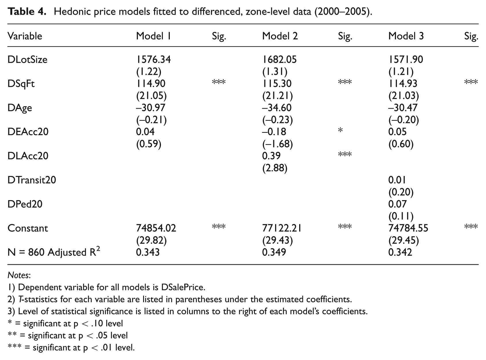
The remaining five specifications from the cross-sectional analysis are repeated using the differenced variables, with the model results reported in Table 4.
Hedonic price models fitted to differenced, zone-level data (2000–2005).
Notes:
1) Dependent variable for all models is DSalePrice.
2) T-statistics for each variable are listed in parentheses under the estimated coefficients.
3) Level of statistical significance is listed in columns to the right of each model’s coefficients.
= significant at p < .10 level
= significant at p < .05 level
= significant at p < .01 level.
The first thing to note when looking at the results of these models is that their overall fit is significantly poorer relative to those fit to the cross-sectional data. Whereas the cross-sectional, zone-level models all produced adjusted-R 2 values of over 0.6, the corresponding values for differenced models are all below 0.35.
Second, the coefficient values on the employment access variables are slightly higher than those produced by the cross-sectional models, but nearly all of them are statistically insignificant at any reasonable threshold of significance. As was done with the cross-sectional models, we also tested higher travel time thresholds. Results indicated higher coefficient values for the 40- and 60-minute employment access (by car) variables, with the latter approaching a marginal level of significance. These results contrast with the estimates from the cross-sectional models, where the employment access variables with higher travel time thresholds produced coefficients with smaller values and no statistical significance. Intriguingly, the accessibility variables in the differenced models are not that different from those in the cross-sectional models in terms of sign and magnitude, despite the former’s larger standard errors. We note the possibility that the lack of statistically significant effects of these variables in the differenced model could be reflective of the model’s inherent weaknesses in addition to the lack of a strong relationship with house price changes.
Third, the results from Model 3, which includes the walking and public transit employment access variables, indicate that none of the modal employment access variables are statistically significant. While all three coefficients carry a positive sign, the associated t-values are all well below a value of 1. This is notable since, unlike the cross-sectional accessibility variables, the variables measuring accessibility change by mode are largely uncorrelated with one another and hence less susceptible to problems of collinearity.
Fourth, the inclusion of a labour accessibility variable (in Model 2) again has a significant effect on the stability of the coefficient for the employment accessibility variable. As Table 4 indicates, the inclusion of the labour accessibility variable causes both it and the employment accessibility variable to have the opposite sign from what was expected. Again, the correlation between these two variables (r = 0.72), even when in differenced form, seems to bias the coefficient estimates.
To summarise, the models predicting changes in house prices as a function of changes in housing attributes and levels of accessibility produce a much poorer fit than the models fit to cross-sectional data. None of the accessibility change variables, regardless of mode, were able to consistently predict changes in house prices. In the next section, we consider what might account for the differences in results across models, and what implications may arise for the conceptual understanding and measurement of the relationship between accessibility, urban structure and land value.
Discussion
The previous section presented the results of analyses of house prices and price changes over time. The differences were stark in terms of model fit and the statistical significance of the variables representing regional accessibility. One possible interpretation of these results is that the models measuring changes in accessibility and house prices over time are more accurately describing the marginal effect of accessibility improvements, and that this effect is indeed too small to be statistically detectable. Why might this conclusion be possible?
The analyses of cross-sectional and differenced data presented here are illustrative of the types of problems associated with the measurement of the relationship between transportation networks and urban structure. Over time, urban structure is influenced by the sequential deployment of transportation networks representing various modes and technologies. A common process of development in many American cities is for parts of the city to reflect an urban structure influenced by the dominant transportation technology of the time, from walking to some form of fixed-route urban transit, and eventually to the automobile (LeRoy and Sonstelie, 1983). But while new modes supplant older, inferior ones, the parts of the city that developed around earlier technologies tend to retain much of their earlier form. The building stock within cities is among the most durable of its features, and so in the older parts of many cities urban structure tends to change relatively little, even over long periods of time. This durability, or ‘vintage effect’ (Brueckner, 1980) helps to explain how even in contemporary urban regions it is possible to find some empirical support for patterns of land rent associated with earlier theories of urban structure, such as the monocentric city (Frew and Jud, 2003; McMillen, 2003).
This effect will also be present when using more disaggregate (zone-based) measures of accessibility, since CBDs and other, more centrally located neighbourhoods in most cities tend to retain large concentrations of activities (i.e. employment), and hence have higher levels of accessibility and land value. The fixity of the building stock and the absence of vacant, developable land in these locations suggest that their overall levels of accessibility are likely to change little, even over significant periods of time. Thus, the relationship between their level of regional accessibility and land prices, all else constant, should be stable over time. Centrally located neighbourhoods, and especially CBDs, also benefit from the tendency of newer transportation networks to provide superior levels of service to central locations within regions. Even highway networks, which are often cited as decentralising forces within regions, tend to have hub-and-spoke route structures that provide the highest levels of accessibility to centrally located areas.
One can think of the deployment of transportation networks within cities as the shape of an ‘S-curve’ or logistic growth curve. 1 This growth curve should accurately characterise the periods of birth, growth and maturity of a transportation network. Within many American cities, as with cities in other developed countries, most transportation networks are at a stage of maturity. The implication is that marginal changes to the network are likely to have at most minor impacts on patterns of accessibility (Gomez-Ibanez, 1985).
Indeed, there are interesting parallels with other strands of literature which raise the question of average versus marginal effects in the deployment of transportation networks. The spate of studies in the economics literature during the late 1980s and early 1990s examining the relationship between aggregate investment in transportation and other ‘core’ infrastructure and economic output illustrate this phenomenon. Prominent reviews of this literature (Gramlich, 1994; Hulten and Schwab, 1993) have emphasised that studies which properly detrend and disaggregate their data reveal evidence of diminishing returns to more recent investment, as do studies which follow such trends over time (Fernald, 1999; Shirley and Winston, 2004).
If a relationship exhibiting diminishing marginal returns to additional network growth within cities does in fact exist, then there are some notable implications one can draw regarding the appropriate functional form to use in empirical models relating accessibility to land value. Most such empirical studies tend to use model specifications that suggest a relationship between accessibility and land value that is either linear or linear in the logarithms of the two variables. While these specifications often yield results that are acceptable in a broad statistical sense, they seem to fail to capture the effect of diminishing marginal returns that is inherent in transportation network deployment. A model specification that uses a logarithmic transformation of only the independent variable may be better able to represent this relationship. Our analysis of the cross-sectional relationship between accessibility and house prices provides some support for this contention.
In addition to the matter of estimating the marginal effects of accessibility improvements, our analysis also raised the issue of whether or not there are residual influences of public transit and pedestrian accessibility on land prices after controlling for access by auto. We have seen few previous studies that have attempted such an analysis. Indeed, the correlation between measures of accessibility by different modes makes such analysis difficult, but our use of differenced variables in the analysis of price changes was able to reduce this source of collinearity to the point where a reasonable model could be specified and estimated. The results indicated that after controlling for changes in accessibility by auto, changes in public transit and pedestrian accessibility did not yield any statistically significant impacts on home prices.
Conclusion
Despite the large amount of attention afforded to studies of the relationship between location and land value, there is still remarkably little evidence on how this relationship evolves over time and space. This paper has sought to provide a point of reference, including a replicable methodology, for investigating the dynamics of this relationship further. We hope that the results and discussion presented here will provoke a critical re-examination of how researchers go about measuring relationships between urban structure, location and land value.
Our findings indicate that some of the relationships between accessibility and house prices that appear in models fitted to cross-sectional data are weakened when measured in terms of changes over time. Some of this may be attributed to the short-term nature of the data set, using only five years of changes to evaluate the relationship. However, another possible interpretation is that the differences in these estimates represent, in a sense, the difference between ‘average’ and ‘marginal’ effects of transportation improvements.
Stated slightly differently, while it is possible to observe high land prices in locations with high accessibility, much of that location premium may have as much to do with the effects of previous generations’ investments as it does more recent ones. An implication for planning practice is that it would also mean that there is little guarantee that current investments in network improvements would be able to match those of previous decades (or longer), or that previous estimates of responses to accessibility changes based on cross-sectional relationships would be a good guide to estimating benefits from current changes. The benefits from current improvements may depend at least partly on the prevailing levels of accessibility provided by the network. This is an important consideration for urban areas in higher-income countries, where networks may already be substantially more mature and built out, providing already-high levels of access. We think this hypothesis is one that is deserving of further investigation.
The ‘representative house’ approach presented here and the limitations of the data sets used to calibrate it suggest some areas for possible improvement if and when this approach is replicated. For instance, one may question whether a five-year period is a long enough slice of time to observe meaningful changes in the components of accessibility, namely the structure of transportation networks and the spatial distribution of activities. Efforts to collect and archive data on these components in future years (especially regional accessibility) may greatly improve the ability to test this relationship over longer periods of time. Our analysis also indicated that models predicting changes over time, as reflected in the differenced specification, yielded a poorer overall statistical fit. The reasons for this may be many, but one distinct possibility is that the relationship between accessibility changes and price changes contains a lag of one or more years, as development patterns respond to new patterns of access. Testing for different adjustment periods may yield more insights into this process.
Other measures could further increase the robustness of the approach. In addition to collecting longer-term data series to allow for longer periods of adjustment to changes in accessibility, future research should try to identify other types of variables reflecting things such as urban amenities or neighbourhood-level attributes which could be measured at a zonal level or aggregated up to it. Also, in order to improve the reliability of the estimates from a zone-level model, certain restrictions could be placed on the number of observed sales in each zone in order to ensure a minimum sample size from which to construct the representative house. Alternative types of accessibility measures, such as those based on the doubly constrained gravity model, could also replace the use of cumulative opportunity measures in order to reduce problems with collinearity when trying to disaggregate the effects of accessibility to employment versus workers.
Another alternative to addressing the weaknesses identified in the representative house approach would be to use a method such as repeat sales to estimate the effects of accessibility changes. This would avoid the need to identify and measure changes in most structural and neighbourhood attributes, since many of them could be assumed to be time-invariant, at least in the shorter term. This method would also allow some flexibility in terms of the scale at which accessibility is measured. It would, however, require longer time series of sales in order to generate a sufficient number of repeat sales.
One other direction in which we suggest expanding this research is the disaggregation of urban areas into smaller study units in order to better estimate the marginal effects of accessibility changes and to reduce one source of heterogeneity in empirical models. The simplest type of disaggregation might be to divide the sample of regional house sales into central city and suburban submarkets. While housing markets are commonly referenced as one of the elements that unify cities as an economic unit, urban economists have keenly observed that there may be important differences in the behaviour of housing submarkets within the same urban area (Goodman and Thibodeau, 2007). One recent study by Habib and Miller (2008) explores the use of market segmentation with a model that simultaneously accounts for spatial and temporal sources of heterogeneity in house prices using clustering techniques to define different neighbourhoods. Combining this type of approach with a more refined, disaggregate representation of location and accessibility would be a good starting point for providing a more detailed understanding of the dynamic relationship between location and land value.
Footnotes
Funding
This research received no specific grant from any funding agency in the public, commercial, or not-for-profit sectors.