
Abstract
Rapid transit projects that increase accessibility should result in a localised land value uplift (LVU) benefit for locations near stations. A rich history of research has tested this hypothesis, generally operationalising transit accessibility by proxy through distance from a transit station. However, a growing body of research has also demonstrated LVU effects from transit-oriented development (TOD) as individuals sort themselves into locations that best match their preferences and willingness to pay. Considering the interdependence of transportation and land use in the urban system, we argue that these benefits create a spatial bundle of TOD goods around transit stations and hypothesise that households are willing to pay a premium for locations in more transit-oriented station catchment areas. Utilising latent class analysis, we quantify station area TOD submarkets. Next, interactions between these submarkets and station proximity in spatial hedonic regressions reveal that TOD is capitalised into land values in Toronto, though the maximum amount and spatial impact area of this capitalisation differs by TOD context.
Introduction
Determining the amount of land value uplift (LVU) produced by rapid transit infrastructure is of great importance as it provides evidence of a project’s larger benefits to society. While such transit projects can be pursued to produce many tangible and intangible benefits (Higgins and Kanaroglou, 2016c), we focus here on two of the most significant ways they can impact the urban land market: through improvements in transportation accessibility and by shaping the built environment around transit stations.
First, accessibility can be defined as the potential for reaching opportunities distributed over space from a particular location while considering the cost or difficulty involved in travelling between them (Páez et al., 2012). The spatial equilibrium framework of Alonso (1964), Muth (1969), and Mills (1972), referred to here as the AMM model, posits that the spatial distribution of transportation costs in terms of time, money, or even stress (e.g. Higgins et al., 2017), are primary drivers of differences in land values over space. If a rapid transit facility can offer a reduction in transportation costs and an improvement in accessibility, land values around stations should increase. Because most transit trips begin and end on foot, the spatial extent of LVU should peak at stations and generally dissipate over a short distance, typically operationalised as a 10-minute walk or about 800 m (Guerra et al., 2012). However, for a rapid transit project to produce LVU from accessibility, it must offer travel benefits relative to other modal options (Higgins and Kanaroglou, 2016b).
Second, the trend towards increasingly coordinated land use and transportation planning for many rapid transit projects can result in additional price effects from transit-oriented development (TOD), which generally refers to a high-density, mixed-use, amenity-rich, and pedestrian-friendly built environment around rapid transit stations. In terms of LVU, the type of lifestyle offered through TOD implementations is said to be particularly valued by specific cohorts of the population, namely young professionals, empty-nesters, and recent immigrants (Cervero et al., 2004; Dittmar et al., 2004), especially in the age of the ‘consumer city’ detailed by Glaeser et al. (2001). Indeed, previous literature has demonstrated positive land value changes associated with aspects of TOD (Bartholomew and Ewing, 2011; Higgins and Kanaroglou, 2016b).
To that end, what does the literature say regarding the LVU impacts of rapid transit? A comprehensive review by Higgins and Kanaroglou (2016b) revealed that in North America alone, more than 100 studies have sought to capture the relationship between rapid transit and land values, and results have been mixed. As the review argues, one reason for this heterogeneity in results is that many previous studies have assumed LVU impacts are derived only from accessibility. This relationship is typically operationalised by proxy through measures of distance from a transit station to capture the peaking in land values the AMM model predicts. From this, studies have often estimated models across a group of adjacent transit stations simultaneously to return ‘global’ estimates of LVU that are interpreted as evidence of an accessibility benefit.
Such an approach is potentially problematic. One of the main issues affecting hedonic models in general is bias introduced from omitted variables in the estimation of the hedonic price function, particularly when such omitted characteristics are correlated with a variable of interest (Kuminoff et al., 2010). For the present research area, a focus only on accessibility ignores the mutually dependent relationship between transportation and urban form in the urban system, where transportation infrastructure affects accessibility, accessibility shapes land use, land use guides travel patterns, and travel patterns influence the provision of transportation infrastructure (Giuliano, 2004). Such interdependency makes it difficult to analyse only one aspect of the urban system in isolation, and means measures of proximity to a transit station risk capturing benefits from transit’s regional accessibility, local station area land use and transit-oriented amenities, or a combination of both. Following Kuminoff et al. (2010), such an approach introduces the potential for omitted variables, unobserved relationships, and potentially misvalued results.
The actual supply of transportation infrastructure and transit-oriented land use development is dependent on a host of factors, such as public expenditures on transit, permissive zoning, and development incentives. But given their fundamental mutual dependence in the urban system, we argue that a rapid transit station area’s accessibility and built environment characteristics combine to result in a spatial basket or bundle of TOD goods around transit stations. Compared with the AMM model’s focus on land price as an outcome of the tradeoff between accessibility and space, our conceptualisation of the LVU benefits of rapid transit projects draws from Tiebout’s (1956) theory of sorting, wherein individuals self-select their location based on the best fit between individual preferences and the characteristics of different areas.
This is not to say that the spatial equilibrium frameworks of the AMM model and Tiebout are incompatible; they are instead complimentary (Epple et al., 2010; Hanushek and Yilmaz, 2007). We argue here that the heterogeneous distribution of different bundles of transit accessibility and transit-oriented built environments over space results in TOD as a location-specific amenity and produces submarkets of TOD characteristics. From this, individuals choose their location based on the utility-bearing attributes of these different TOD bundles, which are defined spatially by a station’s catchment area. If TOD is valued, individuals should be willing to pay a price premium to live in transit-oriented locations.
Not all previous research in this area has been insensitive to the built environment. Some authors control for land use through measures such as population density to better identify accessibility benefits (Higgins and Kanaroglou, 2016b). Similarly, a strand of recent research has sought to capture heterogeneity in LVU by a station’s built environment context. Atkinson-Palombo (2010) used a cluster model of several built environment indicators to tease out what were hypothesised as accessibility benefits from being proximate to rapid transit in different station area contexts. Results show that single detached homes and condominiums were worth 6% and 20% more, respectively, in mixed-use and amenity-rich neighbourhoods while no effect was seen in low-density residential neighbourhoods.
Duncan (2011a, 2011b) opted for an interaction approach to isolate how accessibility as proximity changes with measures of the built environment. Duncan (2011a) for example found that proximity to the San Diego Trolley is worth more in areas with higher densities, walkability, and retail employment. Similarly, Duncan (2011b) found that the value of proximity to Trolley stations is conditional on TOD zoning, with higher prices for single-detached homes with larger lots in areas zoned for higher densities.
The present paper generally continues this line of reasoning but breaks with past studies in three ways. First, rather than view the benefits of rapid transit as a product of accessibility alone, we re-conceptualise transit accessibility and the built environment around stations as an interdependent bundle of TOD goods. Second, instead of the traditional clustering methods utilised by Atkinson-Palombo (2010), we employ latent class analysis (LCA) to arrive at a probabilistic classification of neighbourhood TOD. Finally, we incorporate this classification in our hedonic models and employ interaction terms to isolate the joint effects of TOD and proximity to a station area’s TOD centre of gravity on land values in Toronto, Canada.
Research design
Study area
Toronto has a rich history of using rapid transit to guide growth (Bower, 1979), and the city’s experience with what is now commonly known as TOD has been hailed as an example for other jurisdictions. Knight and Trygg (1977) and Huang (1996) for example note how Toronto has long offered permissive zoning and density bonuses around subway stations, coordinated station design efforts with developers, and even aggressively marketed station air rights for development. While Toronto’s growth has been imperfect (Filion et al., 2006), its long-standing friendliness to coordinated transportation and land use planning presents an ideal opportunity to examine how the different bundles of TOD that have emerged over the past several decades are impacting LVU.
The study area consists of two intersecting Toronto Transit Commission (TTC) heavy rail transit (HRT) lines in the City of Toronto (Figure 1). Line 1 runs north–south and travels into the heart of the city’s central business district. The seven Line 1 stations within the sample have been in service since at least 1974, with Eglinton and Davisville opening in 1954. Line 4 features five stops spread over 5.5 km and feeds into Line 1. With service beginning in November of 2002, it is the city’s most recent HRT line. The study area also includes one commuter rail transit (CRT) station on GO Transit’s Richmond Hill Line, which began operation in 1978 and offers service to the central business district. The station is about 500 m from Leslie subway station and located beneath regional Highway 401. Very few of the transactions outlined below are within walking distance of this station, and zero are within a 10-minute walk of both a TTC and GO station. Nevertheless, we include Oriole GO as a control variable.

Study area and sale transactions.
Research hypotheses
The present paper seeks to test the following hypotheses:
H1: Rapid transit nodal accessibility and the built environment within a rapid transit station’s catchment area combine to present a bundle of goods that reflects different TOD characteristics, and this bundle is heterogeneous over space.
H2: Compared with locations outside of a rapid transit station catchment area, proximity to TOD is associated with an increase in LVU.
H3: Different bundles of TOD are associated with differential rates of LVU, with higher price premiums for locations that are more reflective of TOD as a concept.
H4: Rates of LVU are not time-constant.
Put another way, through H1–H3 we hypothesise that transit accessibility and the built environment are a bundle of goods and that proximity to rapid transit is worth more in areas that are more reflective of TOD as a concept. H4 also hypothesises that rates of LVU change over time, potentially a result of unobserved buyer preferences and broader trends in the local real estate market. In the Toronto context specifically, changes in the value of TOD between 2001–2003 and 2010–2014 could be expected based on two local trends. First, station area TOD has changed as the city has grown in both population and jobs and the new development required to accommodate it. A second factor is that young adults are increasingly moving to higher-density urban locations that are amenity-rich and well-served by public transit, a process Moos (2016) refers to as the ‘youthification’ of Toronto.
Modelling approach
To estimate the capitalisation of different bundles of TOD in the urban land market we utilise hedonic multiple regression with a data set of transacted house prices in a repeat cross-sectional model design. Established by Lancaster (1966) and Rosen (1974), the hedonic method postulates that the value of a good is determined by its utility-bearing attributes, and regressing these attributes on the price of the good can reveal their implicit value at market equilibrium. Isolating the value of land in a cross-sectional model requires the analyst to control for the other characteristics that make up the price of a home and to accomplish this we adopt the hierarchical model structure depicted in Figure 2. Here, variables reflecting structural, location, and time of sale characteristics of the home are regressed on its sale price, which is log-transformed to account for any non-linearities in the hedonic price function.
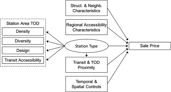
Model structure.
To reveal the capitalisation of TOD into land values, we adopt a two-stage approach with three measures. First, like other models in this research area, we measure a parcel’s proximity to a transit station access and egress point and capture this main effect directly. However, in contrast to other studies, we include a second key variable that controls for the LVU effects of heterogeneous station area TOD contexts. Using LCA, we incorporate a measurement sub-model that distils several attributes of station area TOD into a latent categorical variable corresponding to more homogeneous station types. This categorical variable is used to isolate the value placed on different bundles of TOD characteristics.
Finally, our third key variable consists of an interaction effect between station proximity and the station area TOD variable to account for a home’s proximity to the TOD ‘centre of gravity’ that rapid transit access and egress points provide. Together the three variables account for basic proximity effects common to all station types, a station-type specific TOD effect that should represent the more localised value placed on a location within walking distance of different bundles of TOD characteristics over and above common proximity, and the interaction effect that measures the rate at which the combined common and station-type specific effects decay over space as distance from the station increases.
Latent class TOD model
Transit access and station area TOD context
For the TOD context sub-model, we adopt the methodology proposed by Higgins and Kanaroglou (2016a) for using LCA to distil station area accessibility and built environment characteristics into a typology of different TOD bundles. TOD is operationalised by quantifying the five primary ‘D’ variables proposed by Ewing and Cervero (2010) according to the following definitions. The first ‘D’ is distance to transit, which considers how we define a station’s spatial catchment area. This catchment area is operationalised in two ways: a circular 800 m theoretical buffer around stations that captures its general built environment context, and the functional spatial area covered by a 10-minute walk (at an assumed speed of 1.3 m/s) that captures how each station is used. The input layer for calculating the walk buffers consists of the road network (excluding roads that are not pedestrian accessible) and off-street pedestrian paths mapped by the City of Toronto. Each definition is used as an input to the different TOD measures below. Buffers are unique to each station and not permitted to overlap. Exceptions to this are for adjacent station areas across the CRT and HRT networks and for the buffers used as inputs into the Design variable.
Density consists of population and employment per hectare within each station’s theoretical catchment area. Population and employment counts come from the Canadian Census of Population and the Toronto Employment Survey, respectively, each for the years 2001 and 2011. Diversity is measured in two ways. The first reflects the ratio of employment to population and employment within 800 m to gauge the development mix of each station. A second measure of diversity is land use mix, measured as the proportion of residential, commercial, industrial, and mixed-use land in each 800 m station area for each time period.
Destination accessibility considers a station’s interaction potential as measured by the gravity equation:

where
Finally, Design considers the overall design of the pedestrian network (streets and off-street pedestrian paths) measured through street connectivity. A second set of overlapping theoretical and functional buffers were created, and Design is the ratio of the area contained within a 10-minute walk to that of a circular 800 m buffer. Such an isochronic measure implicitly captures characteristics of the pedestrian shed, such as cul-de-sacs and intersection density. This method is similar to the 10-minute ‘ped-shed’ proposed by Porta and Renne (2005), and combined with our built environment measures, reflects the ‘walkability index’ employed by Frank et al. (2005). While this quantification of the walking environment lacks qualitative indicators, research by Manaugh and El-Geneidy (2011) found that the ped-shed and walkability indices performed as well as or better than the commonly used Walk Score index as correlates of household non-work walking trips.
Each of our TOD measures is quantified in ArcGIS. To increase the accuracy of population and employment estimates, counts at the dissemination area of geography are intersected with population- and employment-oriented parcels of land, respectively. Population, employment, and land use information is apportioned to each station buffer based on the proportion of a polygon intersecting the buffer. Figure 3 offers a visual depiction of this process for land use (Panel A) and population and employment data (Panel B), and this process is repeated for each time period.

Station area detail.
Latent class analysis
Like Ward’s or k-means clustering, LCA is a technique for the unsupervised classification of observations. However, compared with those methods, LCA offers several advantages: it is probabilistic and assumes its latent variable is informed by a mixture of underlying probability distributions; it does not require variables to be standardised and can handle different scales of measurement; it offers the analyst more formal criteria on which to make decisions about the number of classes; and it allows for the post-hoc classification of new observations on an existing cluster solution, a property we utilise here to maintain compatibility with Higgins and Kanaroglou (2016a).
Rather than use the LCA sub-model, the measures of neighbourhood TOD characteristics above could enter the hedonic model directly to reveal their individual implicit prices. However, the mutual dependence of transportation and urban form results in multicollinearity among our measures of TOD (Appendix B) that is problematic for multiple regression. On the other hand, LCA seeks to represent or explain correlations among observed variables through the latent classification so long as model results meet the key assumption of local independence, wherein variables are assumed to be independent of one another within-class after estimation. From this, we argue the LCA sub-model’s latent variable is an effective way of capturing the TOD context of an area to reveal the implicit price of TOD as a spatial bundle of goods.
The two-step estimation of the model depicted in Figure 2 first classifies stations using LCA based on the model’s posterior probabilities and incorporates this classification as an input variable into the spatial hedonic regression. A single-step estimation of the LCA and regression is possible, but per Petras and Masyn (2010), the choice of one- or two-step estimation entails different theoretical implications. A one-step model incorporates the regression as an additional indicator of latent class membership, which in this case would assume house price is another variable characterising the latent classes. In contrast, the two-stage estimation assumes a directional relationship between the latent categorical variable and the exogenous outcome. In our case, the two-step method is preferable as it treats house price as an outcome of the latent TOD context.
Still, while we incorporate LCA to reduce potential bias in the hedonic price function from omitted variables and correlations between accessibility and land use in the urban system, treating a probabilistic LCA classification as observed in the two-step approach can introduce its own bias in the parameters of the second stage regression. There are two potential solutions to this issue. The first is the most-likely class method, which classifies stations based on their highest posterior classification probability. Per Clark and Muthén (2009), the validity of this approach depends on the quality of the LCA classification as measured by the entropy statistic, which ranges from 0 to 1 with a value of 1 implying a perfect separation of classes. Higher entropies, particularly those greater than 0.8, indicate less error in the classification and introduce less potential for bias when most likely class membership is treated as observed and used as an input into additional models.
The second option is the pseudo-class draws technique. As outlined by Petras and Masyn (2010), this method classifies stations based on random samples from their distribution of posterior probabilities in the LCA. A series of random draws (Wang et al. (2005) recommend 20) allows stations to change their class membership and introduces variability in the estimation of the relationship between the latent station type variable and house price in Figure 2. Consistent estimates of the relationship between the mixture of latent classes and the dependent variable are obtained by averaging estimates over the pseudo-class draws.
Hedonic multiple regression
Real estate transaction data
The sample consists of single-detached homes located within 1 km of the selected TTC lines. Transaction data have been obtained over two time periods: 2001–2003, and 2010–2014. For the latter period, this includes records of roughly 2000 transactions. In the earlier period, we utilise a larger data set from Farber and Páez (2007) and Páez et al. (2008), but extract only transactions that occurred within the same geographic study area for a total of roughly 3000. In both cases, data were obtained from the Municipal Property Assessment Corporation, which maintains a database of all properties in Ontario with information on their structural characteristics and assessed and transacted value. The database is linked to Ontario’s geographic parcel fabric and was pre-screened for any sales that were not determined to constitute an open-market transaction.
Structural, parcel, and neighbourhood characteristics
Each transaction record contains several key structural and parcel characteristics associated with the home. Median household income at the dissemination area level of geography is used to act as a proxy for overall neighbourhood characteristics and we also measure a home’s proximity to its nearest park and school. To control for household access to regional job markets on the road network, we employ a second gravity measure of regional interaction potential. The equation is the same as the right-hand side of equation (1), but here the input
Temporal effects
To control for any temporal effects in the real estate market such as seasonal trends, inflation, sales volume, or other factors, we incorporate a series of quarterly dummy variables in the models. Beyond inflation, we hypothesised earlier that LVU associated with TOD is not time-constant, and if any differences over time exist, they should be revealed through changes between time periods in our repeat cross-sectional model design.
Spatial effects
Model diagnostics for aspatial hedonic regressions revealed the existence of spatial autocorrelation. In response, Thiessen polygons for each sale were created, a spatial weights matrix based on a ‘queen’ system of spatial contiguity was calculated, and models were re-run with spatial lag and spatial error terms with heteroskedastic error correction (Kelejian and Prucha, 1998, 1999, 2010) as implemented in the program GeoDa Space. Equations (2) and (3) describe the general form of the spatial lag and error model:
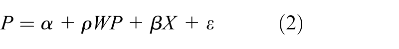
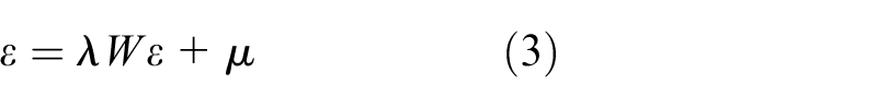
where
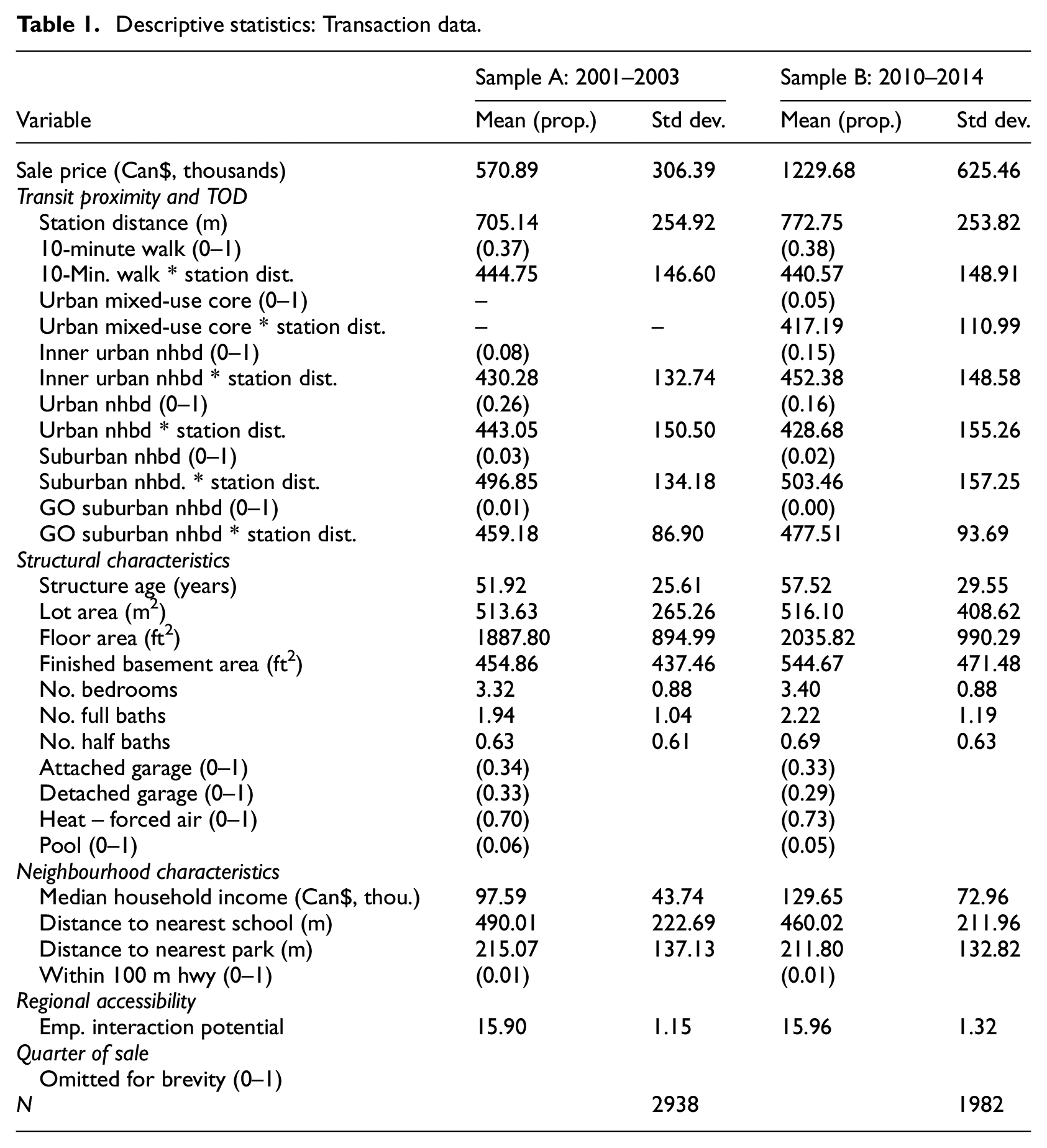
Descriptive statistics
Table 1 displays basic descriptive statistics for the variables included in the hedonic model. Comparing average prices across time periods gives an indication of the price appreciation that has occurred in the region over the past number of years. Table 1 also includes descriptive statistics for the different station types, which are defined and calculated based on a station’s most likely class membership from the LCA model results presented in the next section.
Descriptive statistics: Transaction data.
Model results
Latent class analysis
Using MPLUS 7.2, the latent class model classified each station’s TOD context based on their built environment and transit accessibility characteristics. A typology of station area TOD estimated in Higgins and Kanaroglou (2016a) revealed a best fit with nine distinct types of stations in the Toronto region, with a tenth Airport-type station qualitatively determined. As initial model diagnostics indicated moderate in-class residual covariance between density and accessibility, a covariate relationship between these variables was ultimately specified. The resulting entropy of this classification solution is 0.89, a high value that indicates a clear separation of classes. To keep the station typologies directly comparable, station type membership for the present paper is predicted from this model solution.
The result is a set of four station types within the study area: Urban mixed-use core, Inner urban neighbourhood, Urban neighbourhood, and Suburban neighbourhood. Table 2 displays latent class model results for each station type compared with averages for all stations in Higgins and Kanaroglou (2016a). Here coefficients correspond to each station type’s mean for a given measure of TOD and the significance corresponds to whether this parameter is estimated to be statistically different from zero. Numbers in parentheses reflect the deviation in percentage terms of this value from the sample mean reported in the right-hand column. Also in this column are within-class variances for each class mean. The latent class model assumes variances are constant across classes to ensure the resulting typology of station-area TOD is maximally homogeneous within class and heterogeneous across classes.
Station area TOD characteristics by station type.
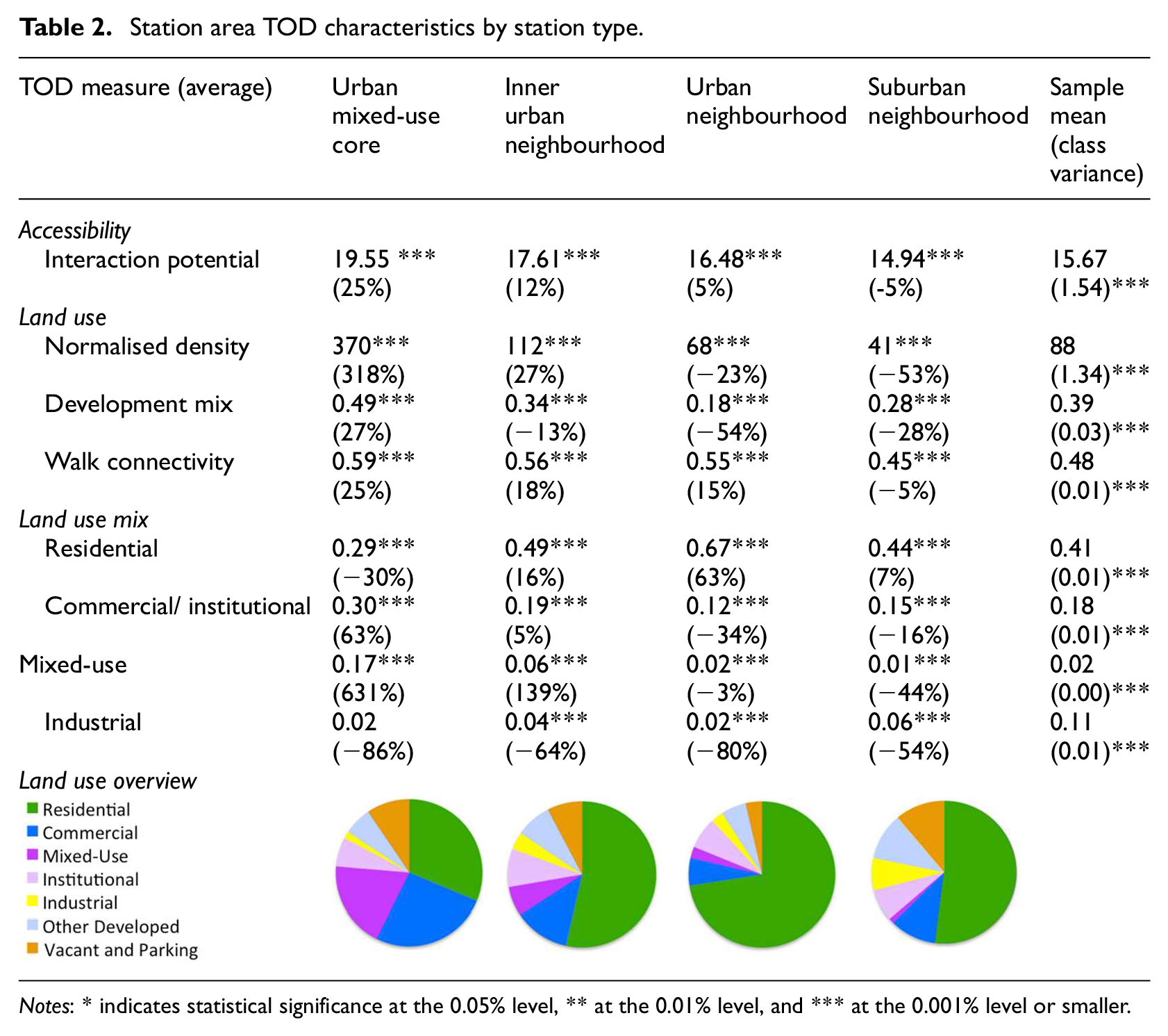
Notes: * indicates statistical significance at the 0.05% level, ** at the 0.01% level, and *** at the 0.001% level or smaller.
Greater discussion of latent class modelling and TOD classification results can be found in Higgins and Kanaroglou (2016a). For the present analysis, results from the typology suggest that Urban mixed-use core and Inner urban neighbourhood stations are most reflective of TOD as a concept, offering the highest levels of transit accessibility and high-density, mixed-use, and pedestrian-friendly development around rapid transit. This generally decreases as stations move from urban to suburban, with Suburban neighbourhoods featuring more homogeneous land uses and lower levels of development intensity, transit accessibility, and pedestrian-friendliness. However, compared with the ten station types in Higgins and Kanaroglou (2016a), all station types in the present study area exhibit of some elements of TOD.
Posterior probabilities for the individual stations are shown in Table 3. Across both time periods, Finch and Lawrence stations for example are clearly classified as an Inner urban neighbourhood and Urban neighbourhood, respectively. However, although the overall entropy for the LCA is high, several stations show variability in their classification and can be characterised by a mixture of station types. The posterior probabilities for Don Mills are roughly split between being an Inner urban neighbourhood and Urban neighbourhood in the early time period, and other stations show moderate mixing across both periods. In response, we adopt the pseudo-class draws technique to minimise potential bias in the second stage of our model.
Sample station posterior probabilities.

Notes: Time period: (A) 2001–2003; (B) 2010–2014. Most likely class for each time period in bold type.
It is also interesting to note that the probabilities for some stations have shifted over time, demonstrating the model’s sensitivity to changes in station area TOD. Eglinton station, for example, evolved from being primarily an Inner urban neighbourhood to a mix between that station type and an Urban mixed-use core as station area population and employment densities, mixed-use land, and accessibility increased. North York Centre, Sheppard-Yonge, and Don Mills stations went from being characterised primarily as Urban neighbourhoods to Inner urban neighbourhoods. In the case of North York Centre, population increased by 61% from nearly 9400 within 800 m in 2001 to more than 15,000 in 2011. For Sheppard-Yonge, population more than doubled to nearly 17,000 while employment totals in both station areas increased by 30%.
Hedonic multiple regression
Results are reported in Table 4 for three sets of models. The first model adopts a traditional structure where the only variable of interest with respect to LVU is a home’s distance from a transit station. The second model advances this specification by considering a separate interacted effect for properties within a 10-minute walk of any station, where a peaking of land values should be more pronounced. In contrast, the third model in each cross section adopts the full interaction approach, where different bundles of TOD are assumed to constitute spatial submarkets that are valued differently by homeowners.
Spatial hedonic model results.
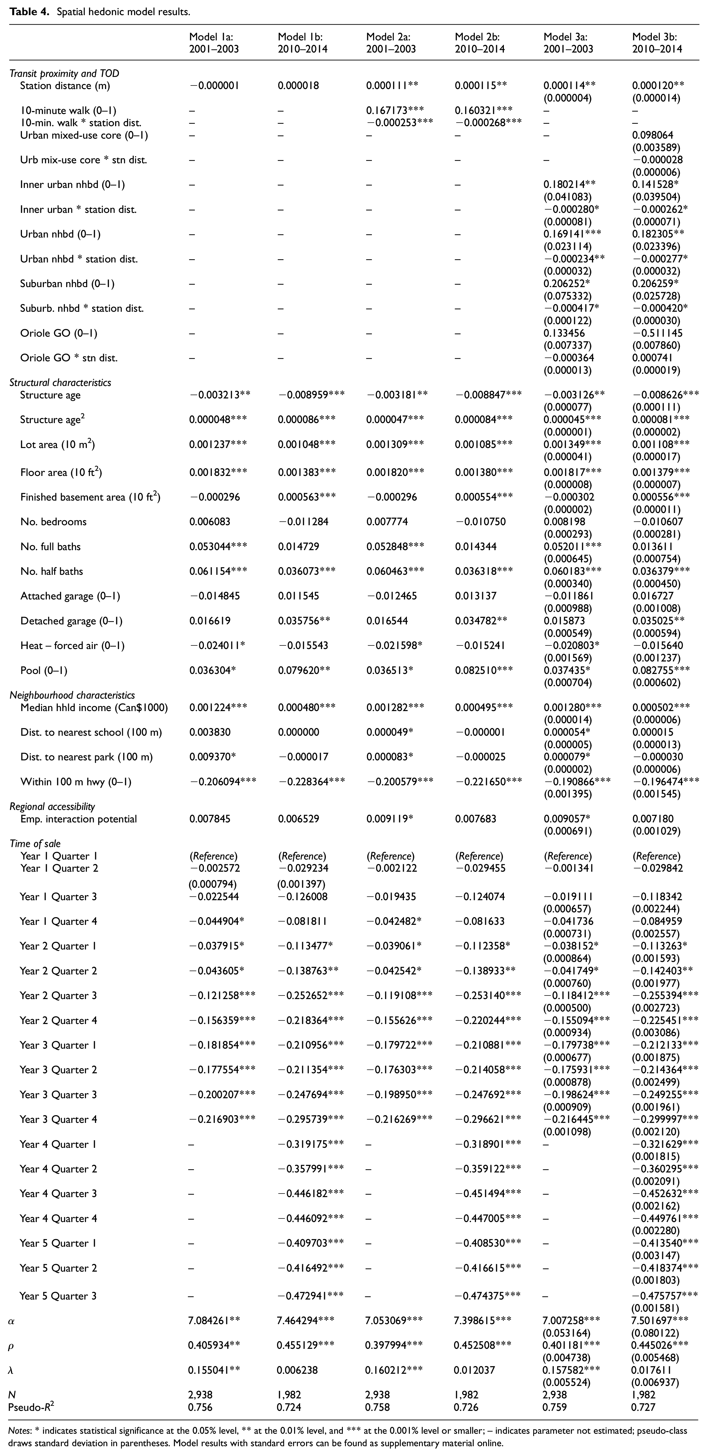
Notes: * indicates statistical significance at the 0.05% level, ** at the 0.01% level, and *** at the 0.001% level or smaller; – indicates parameter not estimated; pseudo-class draws standard deviation in parentheses. Model results with standard errors can be found as supplementary material online.
Model results for the structural, neighbourhood, regional accessibility, and quarterly time of sale control variables generally perform as expected, but for the sake of brevity we omit greater discussion of these impacts. Focusing on the key variables of interest in the Transit proximity and TOD group for Model 1, the lack of statistical significance on the Station distance variable suggests that a home’s proximity to its nearest TTC rapid transit access and egress point is not implicitly priced into the value of land in either cross-section.
However, re-estimation with an interaction specification to capture more localised LVU among properties within a 10-minute walk of a station in Model 2 reveals a strong and significant relationship between price and proximity across both time periods. The reference group consists of homes outside this 10-minute walk buffer. Results indicate that compared with the reference group, a location within a 10-minute walk is associated with a price increase of up to 18% in the early cross-section and 17% in the later cross-section. 1 This effect decreases at a rate of roughly 3% every 100 m further a home is from a station. Compared with Model 1, such results suggest that proximity to the TTC is indeed being priced into the land market and decays in a non-linear fashion as distance from a station increases. However, this global estimate hides any variability by station area TOD context, which the latent class model has shown to be heterogeneous across the study area.
To test whether these LVU amounts are consistent across all station types, Model 3 adopts the pseudo-class draws technique to estimate LVU by station area TOD context. Coefficients reflect the mean value across the 20 draws with standard deviations in parentheses. Although the standard deviations of the Transit proximity and TOD group suggest that different mixes of the stations result in varied estimates of LVU from TOD, the use of the pseudo-class draws method produces consistent estimates of these parameters.
For the earlier time period (Model 3a), compared with the reference group of homes outside a 10-minute walk, a location within an Inner urban neighbourhood station exhibits LVU of up to 20%, decreasing at a rate of 2.8% every 100 m further a home is located from this type of station. For Urban neighbourhood stations, homes are valued up to 18% more than those outside walking distance, decreasing 2.3% every 100 m. Finally, the model estimates that homes located next to Suburban neighbourhood stations are valued at approximately 23% more than the reference group, decreasing rapidly by 4.2% every 100 m further a home is from the station access point. This maximum uplift is 5% greater than the average for all stations in Model 2b.
In the later time period, changes in the character of LVU by station area TOD can be seen. Compared with uplift of up to 20% in the earlier period, the value of living within walking distance of Inner urban neighbourhood stations has dropped to 15%, decreasing by 2.6% every 100 m from a station access/egress point. In contrast, the maximum uplift for Urban neighbourhoods increased to 20%, decaying by 2.7% every 100 m. The premium for Suburban neighbourhoods stayed constant at 23%, again decreasing by 4.2% every 100 m. Interestingly, no statistically significant effect was found for the Urban mixed-use core station type. Similarly, no effect was seen for homes within walking distance of the Oriole GO Suburban neighbourhood station across both time periods.
What about the LVU main effects of proximity to rapid transit? Because of the interaction effects, this coefficient is interpreted differently for homes within and beyond walking distance of a station. For those beyond, it is interpreted as the change in sale price as distance from a station increases. As the results of Models 2 and 3 demonstrate, basic proximity to any type of station is positive, meaning land values for homes beyond walking distance increase as distance from a station increases. However, for homes within walking distance, this coefficient reflects the value of proximity to TOD common to all station types.
Total and net land value uplift
Taken together, the combined effects from the station-type specific TOD, global TOD proximity, and interacted variables capture differential rates of LVU around the sample stations (Figure 4). The panels plot the marginal implicit price derived from Model 3, showing the LVU benefits of TOD as proximity to station access/egress points changes. Panel 1 for example corresponds to Inner urban neighbourhood stations with 1a representing the early time period and 1b the later time period. Using a station’s most likely class membership, we also plot the location of individual sales in the sample to illustrate the distribution of observations informing each curve in the model.
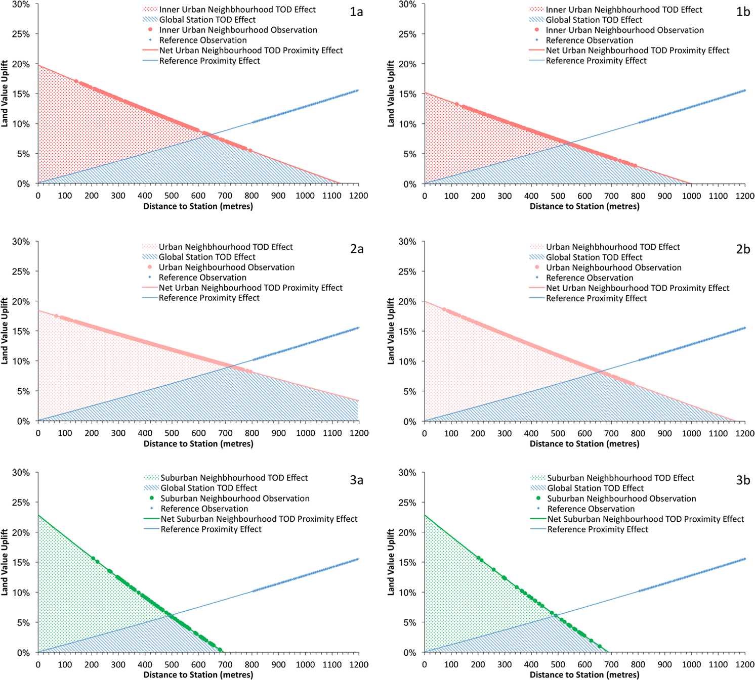
Net land value uplift by station type. 1(a) Inner urban neighbourhood (Sample A); 1(b) Inner urban neighbourhood (Sample B); 2(a) Urban neighbourhood (Sample A); 2(b) Urban neighbourhood (Sample B); 3(a) Suburban neighbourhood (Sample A); 3(b) Suburban neighbourhood (Sample B).
For 1a, total uplift for land within an Inner urban neighbourhood station type is the sum of the three LVU measures. The first is the station-specific TOD effect, which produces a maximum uplift of 20%. Second, the station-specific TOD distance interaction causes this effect to dissipate to zero at 640 m from the station. After this, the global TOD effect common to all station types is estimated to reach zero at 1120 m from Inner urban neighbourhood stations.
However, in terms of net LVU in the urban land market, the global TOD effect is cancelled out by the proximity curve estimated for the reference group of properties beyond walking distance of any station, which begins at 0% and increases to 15% at 1200 m. From this, the three measures of total LVU from TOD and the reference group proximity effect come together to reveal an inflection point in the distribution of land values over space around this type of station.
For Inner urban neighbourhoods in the later cross-section, Panel 1b shows that net LVU decreases in magnitude and spatial extent, with the TOD effect dissipating to zero at 530 m. A different trend can be seen for Urban neighbourhoods in panels 2a and 2b, the latter of which shows that LVU for this station type became more peaked over time. Although the maximum uplift increased from 18% to 20% over cross-sections, the net LVU impact area from station-type specific TOD decreased from within 720 m in the early time period to 650 m in the later time period. Finally, net uplift for Suburban neighbourhoods starts higher than the other station types at 23% in 3a, but the LVU from station-type specific TOD dissipates by 490 m. In contrast to the other station types, net uplift for Suburban neighbourhoods remains unchanged over time periods.
Considering these results, it is interesting to note that the net uplift impact area for land proximate to each of the station types is less than the 800 m/10-minute walk catchment area specified. Similarly, a lack of observations in close proximity to station access and egress points, particularly for Suburban neighbourhoods, means the model is predicting LVU for locations in the immediate vicinity of stations.
Moreover, it should also be noted that the figures above reflect only the direct LVU effects derived from the station distance and station-type variables. In a spatial lag model specification, any amenity benefits at one location exert additional spillover effects on neighbouring properties, which in turn yield added effects on the first property (Kim et al., 2003; Small and Steimetz, 2012). From this, the spatial multiplier approach utilises the model’s spatial lag coefficient to capture any additional indirect spillover effects, and the total value of an amenity is the sum of these direct and indirect effects.
In the present case, the spatial multiplier would increase our estimates of LVU by approximately 67% in the early time period and 80% in the later time period. However, as Small and Steimetz (2012) argue, the use of the spatial multiplier approach is only appropriate if the benefits of an amenity are technological (e.g. a homeowner’s utility increases from their neighbour’s higher property values that result from the amenity) rather than pecuniary in nature. In the present case, any spillover value added by a neighbour’s house being proximate to TOD should not increase a homeowner’s utility above and beyond their own proximity. From this, we conceptualise LVU from TOD as pecuniary and welfare-neutral and focus on only the direct effects.
Discussion
TOD bundles and LVU submarkets
The results confirm several of our hypotheses as they relate to LVU from TOD in the Toronto region. First, latent class model results reveal that station area TOD characteristics vary within the study area, confirming H1. Incorporating the latent TOD classes into the hedonic regression in Model 3 suggests that land in transit-oriented locations is valued higher than land outside station catchment areas, supporting H2. Further-more, different bundles of TOD are priced into single-detached homes at different rates. This partially confirms H3 that LVU effects are heterogeneous and vary by station context. Finally, the changes for Inner urban and Urban neighbourhoods over cross-sections plotted in Figure 4 partially confirm H4 that there are differences in the capitalisation of TOD over time. From this, we can conclude that TOD matters, and different bundles of each are priced into the value of land around rapid transit stations in Toronto.
Nevertheless, the results raise important questions as the directionality of the relationship between TOD and land values in hypothesis H3, where we posited that a greater premium should be found for locations higher in TOD, is not confirmed. Compared with more Urban-type stations, Suburban neighbourhoods are lower in our measured TOD attributes but were found to have consistently higher rates of maximum LVU. That no statistically significant LVU was detected for the Urban mixed-use core station type in Model 3b also appears counter-intuitive as this type of station best represents TOD as a concept in the study area. Furthermore, Inner urban neighbourhoods saw a decrease in maximum LVU over the time periods while Urban neighbourhoods saw an increase and Suburban neighbourhoods stayed constant. Such findings appear to suggest that high intensity TOD is a disamenity to buyers of single-detatched homes.
On the other hand, the net spatial LVU impact from TOD varied by station type with the largest uplift areas for the more transit-oriented Inner urban and Urban neighbourhoods, which suggests that the amenities offered by station areas higher in TOD cast a longer LVU ‘shadow’. That said, in all cases, the net LVU catchment area implied by the models is smaller than our specification of a catchment area as the distance covered by a 10-minute walk.
What might explain these trends? One factor limiting the robustness of the results for the Urban mixed-use core station type in particular is sample size. With only one, it may be that the idiosyncrasies of Eglinton station beyond its measured TOD characteristics are affecting the significance of the station-type specific TOD effects measured by the LCA model.
Related to this, a second likely factor impacting the relationship between TOD and land values is unobserved heterogeneity in individual preferences, which can inform the sorting process into different housing types and TOD submarkets. For Eglinton, the intense development seen around the station over the study period is likely associated with increasing noise, construction, or building shadows, which could in turn be viewed negatively among single-detached homebuyers. Similar development trends are behind the shift in class probabilities for three other stations that switched from being primarily Urban to Inner urban neighbourhoods, which may explain the drop in LVU seen for this station type across time periods.
As in other papers, different results could be found for additional property types, such as condominiums. However, such reasoning assumes property type is a proxy through which significant differences in underlying preferences for TOD among homebuyers are implicitly operationalised. This exposes a fundamental limitation of transaction data; although factors such as a preference for more environmentally friendly lifestyles or the ‘youthification’ of Toronto outlined by Moos (2016) may be impacting real estate values in the study area, transactions alone cannot reveal how the characteristics of the people buying the homes are affecting the observed LVU trends.
Conclusion
With the shift towards integrated transportation and land use planning for rapid transit, it seems plausible that both rapid transit and associated TOD can result in significant price premiums for locations around stations. But previous research into rapid transit’s LVU effects has generally worked from the lens of the AMM model, often estimating models across several stations simultaneously and interpreting any proximity effects as evidence of the capitalisation of accessibility into land. This approach risks leaving information on how LVU varies by station area TOD context unobserved. It also introduces the potential for omitted variable bias in the estimation of the hedonic price function as built environment characteristics can be correlated with proximity to rapid transit.
In response, we explicitly recognise the potential for LVU effects from both transit accessibility and transit-oriented built environments and conceptualise these effects as a bundle of TOD goods spatially defined by the area within a 10-minute walk of a station. Results from the latent class model show that station areas are indeed heterogeneous with respect to TOD. From this, hedonic model results confirm that there are submarkets of LVU effects from TOD in the study area, and that land values decrease as distance from the TOD centre of gravity increases.
Still, although the hedonic model can theoretically isolate the value of land at a certain location, what this land is used for and the preferences of the user affect this value. Our results raise questions related to how different levels of TOD are valued by buyers of single-detached homes: uplift around suburban implementations of TOD is more peaked and decreases rapidly, uplift for stations higher in TOD is flatter with a larger spatial impact area, and there is no effect for the highest intensity TOD. This suggests a complex relationship between TOD and single-detached home values, one where TOD is valued but only up to a point.
Such results offer some direction for research, planning, and policy. First, the finding that TOD is valued in the urban land market shows that households are willing to pay for more sustainable patterns of development, reinforcing Duncan’s (2011a) conclusion that planners should seek to remove supply constraints on TOD. However, like the work of Atkinson-Palombo (2010), our results also suggest that TOD planning and policy may have differential impacts for different housing types proximate to stations. Second, the spatial capitalisation of TOD varies by station type, and in all cases the net uplift area is smaller than the 800 m or 10-minute walk typically used to define a station catchment area. Finally, the contextual sensitivity of LVU means that both transit access and built environment factors should be considered when estimating uplift for existing transit infrastructure, and forecasting uplift for the purposes of land value capture.
However, to offer better guidance on these issues, further study is required. A larger sample of stations and station types would help to increase the robustness of these results, particularly as they relate to our findings for the Urban mixed-use core station type. Researchers should also perform a sensitivity analysis on the assumed spatial extent of a station’s LVU impact area. Moreover, other housing types should be considered, as such buyers may on average place a higher value on TOD, which could in turn result in differences in the magnitude and extent of LVU.
To that end, while our observed LVU estimates reflect the underlying transportation, land use, economic, social, and institutional conditions of the Toronto market, the methods utilised in this paper are generalisable. This includes conceptualising TOD as a bundle of goods, capturing variations in TOD through LCA, and incorporating these measures into spatial hedonic models through the pseudo-class draws approach. The results of the station typology in Higgins and Kanaroglou (2016a) in particular can be utilised within LCA to construct station classifications in other study areas that are directly comparable with the present work.
That said, transaction data alone cannot reveal how implicit homebuyer preferences and broader societal trends are informing the identified LVU curves from TOD. Considering this, future research should seek to analyse the relationship between heterogeneous individual and household preferences, their spatial and household-type sorting decisions, and TOD. Only then can we begin to truly isolate the contextual sensitivity inherent in the relationship between TOD and LVU.
Footnotes
Appendix A
Correlation matrix of TOD measures (later time period).
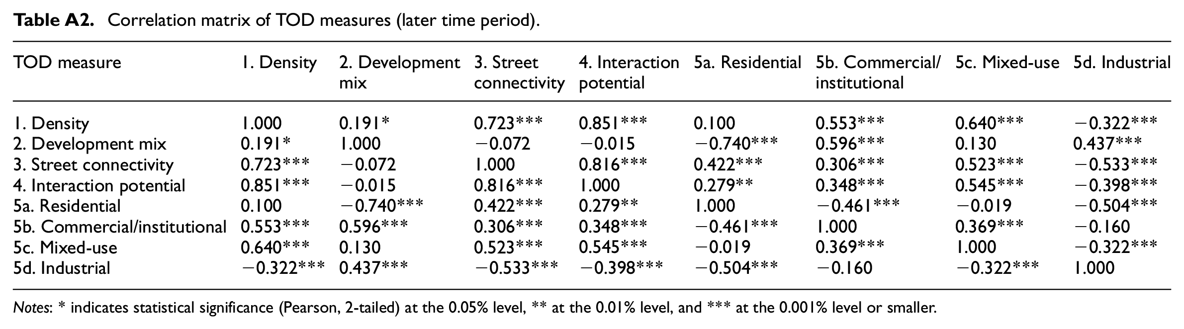
| TOD measure | 1. Density | 2. Development mix | 3. Street connectivity | 4. Interaction potential | 5a. Residential | 5b. Commercial/ institutional | 5c. Mixed-use | 5d. Industrial |
|---|---|---|---|---|---|---|---|---|
| 1. Density | 1.000 | 0.191* | 0.723*** | 0.851*** | 0.100 | 0.553*** | 0.640*** | −0.322*** |
| 2. Development mix | 0.191* | 1.000 | −0.072 | −0.015 | −0.740*** | 0.596*** | 0.130 | 0.437*** |
| 3. Street connectivity | 0.723*** | −0.072 | 1.000 | 0.816*** | 0.422*** | 0.306*** | 0.523*** | −0.533*** |
| 4. Interaction potential | 0.851*** | −0.015 | 0.816*** | 1.000 | 0.279** | 0.348*** | 0.545*** | −0.398*** |
| 5a. Residential | 0.100 | −0.740*** | 0.422*** | 0.279** | 1.000 | −0.461*** | −0.019 | −0.504*** |
| 5b. Commercial/institutional | 0.553*** | 0.596*** | 0.306*** | 0.348*** | −0.461*** | 1.000 | 0.369*** | −0.160 |
| 5c. Mixed-use | 0.640*** | 0.130 | 0.523*** | 0.545*** | −0.019 | 0.369*** | 1.000 | −0.322*** |
| 5d. Industrial | −0.322*** | 0.437*** | −0.533*** | −0.398*** | −0.504*** | −0.160 | −0.322*** | 1.000 |
Notes: * indicates statistical significance (Pearson, 2-tailed) at the 0.05% level, ** at the 0.01% level, and *** at the 0.001% level or smaller.
Appendix B
Spatial hedonic model results with standard errors.

| Model 1a: 2001–2003 | Model 1b: 2010–2014 | Model 2a: 2001–2003 | Model 2b: 2010–2014 | Model 3a: 2001–2003 |
Model 3b: 2010–2014 |
|||
|---|---|---|---|---|---|---|---|---|
| Variable | Coefficient (std err.) | Coefficient (std err.) | Coefficient (std err.) | Coefficient (std err.) | Mean coefficient (std err.) | Std dev. | Mean coefficient (std err.) | Std dev. |
| Transit proximity and TOD | ||||||||
| Station distance (m) | −0.000001 | 0.000018 | 0.000111** | 0.000115** | 0.000114 | 0.000004** | 0.000120 | 0.000014** |
| (0.000020) | (0.000024) | (0.000035) | (0.000043) | (0.000035) | 0.000000 | (0.000044) | 0.000002 | |
| 10-minute walk (0–1) | – | – | 0.167173*** | 0.160321*** | – | – | ||
| (0.039542) | (0.045991) | |||||||
| 10-min. walk * station dist. | – | – | −0.000253*** | −0.000268*** | – | – | ||
| (0.000063) | (0.000074) | |||||||
| Urban mixed-use core (0–1) | – | – | – | – | – | 0.098064 | 0.003589 | |
| (0.080549) | 0.000197 | |||||||
| Urb mix-use core * stn dist. | – | – | – | – | – | −0.000028 | 0.000006 | |
| (0.000176) | 0.000000 | |||||||
| Inner urban nhbd (0–1) | – | – | – | – | 0.180214 | 0.041083** | 0.141528 | 0.039504* |
| (0.057243) | 0.004053 | (0.056354) | 0.004290 | |||||
| Inner urban * station dist. | – | – | – | – | −0.000280 | 0.000081* | −0.000262 | 0.000071* |
| (0.000109) | 0.000010 | (0.000103) | 0.000014 | |||||
| Urban nhbd (0–1) | – | – | – | – | 0.169141 | 0.023114*** | 0.182305 | 0.023396** |
| (0.044640) | 0.002657 | (0.059145) | 0.004428 | |||||
| Urban nhbd. * station dist. | – | – | – | – | −0.000234 | 0.000032** | −0.000277 | 0.000032* |
| (0.000075) | 0.000006 | (0.000105) | 0.000011 | |||||
| Suburban nhbd (0–1) | – | – | – | – | 0.206252 | 0.075332* | 0.206259 | 0.025728* |
| (0.094826) | 0.022273 | (0.089238) | 0.007943 | |||||
| Suburb. nhbd * station dist. | – | – | – | – | −0.000417 | 0.000122* | −0.000420 | 0.000030* |
| (0.000175) | 0.000036 | (0.000162) | 0.000023 | |||||
| GO suburb. nhbd (0–1) | – | – | – | – | 0.133456 | 0.007337 | −0.511145 | 0.007860 |
| (0.102821) | 0.000441 | (0.695486) | 0.001845 | |||||
| GO sub. nhbd * stn dist. | – | – | – | – | −0.000364 | 0.000013 | 0.000741 | 0.000019 |
| (0.000222) | 0.000001 | (0.001205) | 0.000002 | |||||
| Structural characteristics | ||||||||
| Structure age | −0.003213** | −0.008959*** | −0.003181** | −0.008847*** | −0.003126 | 0.000077** | −0.008626 | 0.000111*** |
| (0.001076) | (0.000898) | (0.001076) | (0.000898) | (0.001079) | 0.000001 | (0.000903) | 0.000003 | |
| Structure age2 | 0.000048*** | 0.000086*** | 0.000047*** | 0.000084*** | 0.000045 | 0.000001*** | 0.000081 | 0.000002*** |
| (0.000011) | (0.000009) | (0.000011) | (0.000009) | (0.000011) | 0.000000 | (0.000009) | 0.000000 | |
| Lot area (10 m2) | 0.001237*** | 0.001048*** | 0.001309*** | 0.001085*** | 0.001349 | 0.000041*** | 0.001108 | 0.000017*** |
| (0.000349) | (0.000239) | (0.000350) | (0.000251) | (0.000350) | 0.000002 | (0.000264) | 0.000007 | |
| Floor area (10 ft2) | 0.001832*** | 0.001383*** | 0.001820*** | 0.001380*** | 0.001817 | 0.000008*** | 0.001379 | 0.000007*** |
| (0.000136) | (0.000127) | (0.000136) | (0.000126) | (0.000136) | 0.000000 | (0.000127) | 0.000000 | |
| Finished basement area (10 ft2) | −0.000296 | 0.000563*** | −0.000296 | 0.000554*** | −0.000302 | 0.000002 | 0.000556 | 0.000011*** |
| (0.000160) | (0.000166) | (0.000160) | (0.000165) | (0.000160) | 0.000000 | (0.000166) | 0.000000 | |
| No. bedrooms | 0.006083 | −0.011284 | 0.007774 | −0.010750 | 0.008198 | 0.000293 | −0.010607 | 0.000281 |
| (0.006972) | (0.009128) | (0.006952) | (0.009119) | (0.006946) | 0.000009 | (0.009112) | 0.000020 | |
| No. full baths | 0.053044*** | 0.014729 | 0.052848*** | 0.014344 | 0.052011 | 0.000645*** | 0.013611 | 0.000754 |
| (0.008265) | (0.008314) | (0.008244) | (0.008345) | (0.008260) | 0.000022 | (0.008390) | 0.000034 | |
| No. half baths | 0.061154*** | 0.036073*** | 0.060463*** | 0.036318*** | 0.060183 | 0.000340*** | 0.036379 | 0.000450*** |
| (0.007917) | (0.010127) | (0.007923) | (0.010089) | (0.007912) | 0.000030 | (0.010162) | 0.000024 | |
| Attached garage (0–1) | −0.014845 | 0.011545 | −0.012465 | 0.013137 | −0.011861 | 0.000988 | 0.016727 | 0.001008 |
| (0.012387) | (0.014631) | (0.012406) | (0.014571) | (0.012467) | 0.000014 | (0.014539) | 0.000034 | |
| Detached garage (0–1) | 0.016619 | 0.035756** | 0.016544 | 0.034782** | 0.015873 | 0.000549 | 0.035025 | 0.000594** |
| (0.009572) | (0.013484) | (0.009552) | (0.013490) | (0.009565) | 0.000021 | (0.013524) | 0.000036 | |
| Heat – forced air (0–1) | −0.024011* | −0.015543 | −0.021598* | −0.015241 | −0.020803 | 0.001569* | −0.015640 | 0.001237 |
| (0.010105) | (0.014568) | (0.010051) | (0.014535) | (0.010043) | 0.000044 | (0.014656) | 0.000071 | |
| Pool (0–1) | 0.036304* | 0.079620** | 0.036513* | 0.082510*** | 0.037435 | 0.000704* | 0.082755 | 0.000602*** |
| (0.018139) | (0.024326) | (0.018226) | (0.024085) | (0.018188) | 0.000051 | (0.024273) | 0.000049 | |
| Neighbourhood characteristics | ||||||||
| Median hhld income (Can$1000) | 0.001224*** | 0.000480*** | 0.001282*** | 0.000495*** | 0.001280 | 0.000014*** | 0.000502 | 0.000006*** |
| (0.000166) | (0.000106) | (0.000166) | (0.000106) | (0.000167) | 0.000001 | (0.000107) | 0.000001 | |
| Dist. to nearest school (100 m) | 0.003830 | 0.000000 | 0.000049* | −0.000001 | 0.000054 | 0.000005* | 0.000015 | 0.000013 |
| (0.000024) | (0.000025) | (0.000024) | (0.000025) | (0.000024) | 0.000000 | (0.000027) | 0.000001 | |
| Dist. to nearest park (100 m) | 0.009370* | −0.000017 | 0.000083* | −0.000025 | 0.000079 | 0.000002* | −0.000030 | 0.000006 |
| (0.000038) | (0.000043) | (0.000038) | (0.000044) | (0.000038) | 0.000000 | (0.000044) | 0.000000 | |
| Within 100 m hwy (0–1) | −0.206094*** | −0.228364*** | −0.200579*** | −0.221650*** | −0.190866 | 0.001395*** | −0.196474 | 0.001545*** |
| (0.053116) | (0.047303) | (0.052610) | (0.045421) | (0.056285) | 0.000295 | (0.055746) | 0.000403 | |
| Regional accessibility | ||||||||
| Emp. interaction potential | 0.007845 | 0.006529 | 0.009119* | 0.007683 | 0.009057 | 0.000691* | 0.007180 | 0.001029 |
| (0.004023) | (0.004087) | (0.004012) | (0.004008) | (0.004074) | 0.000057 | (0.004111) | 0.000093 | |
| Time of sale | ||||||||
| Year 1 Quarter 1 | (Reference) | (Reference) | (Reference) | (Reference) | (Reference) | (Reference) | ||
| Year 1 Quarter 2 | −0.002572 | −0.029234 | −0.002122 | −0.029455 | −0.001341 | 0.000794 | −0.029842 | 0.001397 |
| (0.017348) | (0.052238) | (0.017309) | (0.052591) | (0.017307) | 0.000040 | (0.052711) | 0.000156 | |
| Year 1 Quarter 3 | −0.022544 | −0.126008 | −0.019435 | −0.124074 | −0.019111 | 0.000657 | −0.118342 | 0.002244 |
| (0.018226) | (0.071362) | (0.018153) | (0.071277) | (0.018171) | 0.000018 | (0.073574) | 0.000444 | |
| Year 1 Quarter 4 | −0.044904* | −0.081811 | −0.042482* | −0.081633 | −0.041736 | 0.000731 | −0.084959 | 0.002557 |
| (0.021277) | (0.068039) | (0.021251) | (0.067934) | (0.021291) | 0.000033 | (0.067779) | 0.000116 | |
| Year 2 Quarter 1 | −0.037915* | −0.113477* | −0.039061* | −0.112358* | −0.038152 | 0.000864* | −0.113263 | 0.001593* |
| (0.018242) | (0.046187) | (0.018215) | (0.046457) | (0.018177) | 0.000036 | (0.046804) | 0.000180 | |
| Year 2 Quarter 2 | −0.043605* | −0.138763** | −0.042542* | −0.138933** | −0.041749 | 0.000760* | −0.142403 | 0.001977** |
| (0.017398) | (0.047819) | (0.017405) | (0.047135) | (0.017434) | 0.000020 | (0.046925) | 0.000196 | |
| Year 2 Quarter 3 | −0.121258*** | −0.252652*** | −0.119108*** | −0.253140*** | −0.118412 | 0.000500*** | −0.255394 | 0.002723*** |
| (0.018310) | (0.055874) | (0.018290) | (0.056508) | (0.018343) | 0.000016 | (0.056523) | 0.000149 | |
| Year 2 Quarter 4 | −0.156359*** | −0.218364*** | −0.155626*** | −0.220244*** | −0.155094 | 0.000934*** | −0.225451 | 0.003086*** |
| (0.020745) | (0.037257) | (0.020756) | (0.037296) | (0.020736) | 0.000052 | (0.037387) | 0.000094 | |
| Year 3 Quarter 1 | −0.181854*** | −0.210956*** | −0.179722*** | −0.210881*** | −0.179738 | 0.000677*** | −0.212133 | 0.001875*** |
| (0.022494) | (0.035377) | (0.022421) | (0.035471) | (0.022366) | 0.000031 | (0.035503) | 0.000094 | |
| Year 3 Quarter 2 | −0.177554*** | −0.211354*** | −0.176303*** | −0.214058*** | −0.175931 | 0.000878*** | −0.214364 | 0.002499*** |
| (0.017982) | (0.035876) | (0.018000) | (0.035917) | (0.018004) | 0.000018 | (0.036149) | 0.000070 | |
| Year 3 Quarter 3 | −0.200207*** | −0.247694*** | −0.198950*** | −0.247692*** | −0.198624 | 0.000909*** | −0.249255 | 0.001961*** |
| (0.020145) | (0.041969) | (0.020130) | (0.041888) | (0.020151) | 0.000018 | (0.041932) | 0.000153 | |
| Year 3 Quarter 4 | −0.216903*** | −0.295739*** | −0.216269*** | −0.296621*** | −0.216445 | 0.001098*** | −0.299997 | 0.002120*** |
| (0.026673) | (0.037660) | (0.026647) | (0.037652) | (0.026636) | 0.000054 | (0.037630) | 0.000089 | |
| Year 4 Quarter 1 | – | −0.319175*** | – | −0.318901*** | – | −0.321629 | 0.001815*** | |
| (0.035180) | (0.035223) | (0.035180) | 0.000077 | |||||
| Year 4 Quarter 2 | – | −0.357991*** | – | −0.359122*** | – | −0.360295 | 0.002091*** | |
| (0.038229) | (0.038230) | (0.037760) | 0.000081 | |||||
| Year 4 Quarter 3 | – | –0.446182*** | – | −0.451494*** | – | −0.452632 | 0.002162*** | |
| (0.039637) | (0.039730) | (0.039730) | 0.000099 | |||||
| Year 4 Quarter 4 | – | −0.446092*** | – | −0.447005*** | – | −0.449761 | 0.002280*** | |
| (0.040093) | (0.040233) | (0.040342) | 0.000122 | |||||
| Year 5 Quarter 1 | – | −0.409703*** | – | −0.408530*** | – | −0.413540 | 0.003147*** | |
| (0.036347) | (0.036480) | (0.036541) | 0.000098 | |||||
| Year 5 Quarter 2 | – | −0.416492*** | – | −0.416615*** | – | −0.418374 | 0.001803*** | |
| (0.036269) | (0.036252) | (0.036218) | 0.000087 | |||||
| Year 5 Quarter 3 | – | −0.472941*** | – | −0.474375*** | – | −0.475757 | 0.001581*** | |
| (0.040917) | (0.040853) | (0.040971) | 0.000093 | |||||
|
|
7.084261** | 7.464294*** | 7.053069*** | 7.398615*** | 7.007258 | 0.053164*** | 7.501697 | 0.080122*** |
| (0.333625) | (0.375564) | (0.333373) | (0.373449) | (0.336796) | 0.002817 | (0.383563) | 0.005474 | |
|
|
0.405934** | 0.455129*** | 0.397994*** | 0.452508*** | 0.401181 | 0.004738*** | 0.445026 | 0.005468*** |
| (0.026982) | (0.028560) | (0.027077) | (0.028624) | (0.027398) | 0.000276 | (0.029392) | 0.000407 | |
|
|
0.155041** | 0.006238 | 0.160212*** | 0.012037 | 0.157582 | 0.005524*** | 0.017611 | 0.006937 |
| (0.040023) | (0.049015) | (0.039802) | (0.048774) | (0.039961) | 0.000133 | (0.049440) | 0.000146 | |
| N | 2,938 | 1,982 | 2,938 | 1,982 | 2,938 | 1,982 | ||
| Pseudo-R2 | 0.756 | 0.724 | 0.758 | 0.726 | 0.759 | 0.727 | ||
Notes: * indicates statistical significance at the 0.05% level, ** at the 0.01% level, and *** at the 0.001% level or smaller; – indicates parameter not estimated; standard errors in parentheses.
Acknowledgements
The corresponding author would like to extend his gratitude to Pavlos Kanaroglou, who was a mentor and friend up to his passing in May of 2016. The corresponding author would also like to thank the anonymous referees, as their suggestions have helped to improve this paper.
Funding
This research received no specific grant from any funding agency in the public, commercial, or not-for-profit sectors.