Expanding cities and vehicle use in India: Differing impacts of built environment factors on scooter and car use in Mumbai

Abstract

Expanding urban populations are inducing development at the edges of Indian cities, given the constraints on land use intensification within municipal boundaries. Existing peripheral towns are becoming anchors for this new growth, creating urban agglomerations. Such areas have become preferred home locations for the working poor and emergent middle class, groups that are often priced out of the urban housing market. However, many such exurban locations lack infrastructure such as durable paved roads and transit, because investments are largely clustered within municipal boundaries. This paper focuses on the Greater Mumbai Region and relies on a cross-sectional household travel survey data set. The objective is to understand how vehicle use is linked to the built environment and socio-economics. Spatial analysis shows that cars are used in urban centres while scooters and motorcycles are used in the exurbs. Estimated censored regression models show that greater household distance from the main employment centre Nariman Point, better job accessibility and improved socio-economic factors increase vehicle use, while land use diversity and density bring down vehicle use. A key econometric result is that after controlling for location, land use, infrastructure supply and socio-economics, the expectation of a motorised two-wheeler or car in a household does not translate to its use. Overall, the findings suggest that policies encouraging higher land use diversity, density and transit supply have the potential to marginally decrease vehicle use in the Indian metropolis. However, future research needs to focus on residential location to better understand how the choices of where to live and how to travel are interconnected.

Keywords

built environment car motorised two-wheeler South and Southeast Asia vehicle use

Introduction

Growing cities have a tendency to expand outward, with private vehicle use increasing for households locating in the peripheries. This verdict is largely based on transportation scholarship from developed world cases where there is adequate infrastructure supply in the city peripheries. This pattern of higher private vehicle use in the peripheries is also observed in the developing world, though under different conditions. For example, infrastructure production lags behind land development in India, so Indian cities grow rapidly but the supply of roads and transit services is often weak. The need for more infrastructure has been recognised for some time in India (Government of India, 2011), and countrywide polices have been put in place. Specifically, the Jawaharlal Nehru National Urban Renewal Mission (JnNURM), an infrastructure policy for urban India, was in effect between 2005 and 2014. Of the total budget, 14% was spent on urban roads and overpasses, and 8% on other urban transport infrastructure including mass rapid transport systems (Government of India, 2012). However, most of this transportation infrastructure has been supplied in urban centres, while the exurbs have seen marginal investments. One consequence of the relatively small level of expenditure for urban mass transportation is that service levels are often poor, especially at the peripheries of cities.

While middle class and affluent groups generally live in suburbs in the developed world and have access to good infrastructure, working poor and emergent middle class households (Shirgaokar, 2014: 249) live in the peripheries of Indian cities; the well-off live in the expensive urban centres. Households that locate in the exurbs tend to be upwardly mobile and seek a better quality of life. The well-off city-centre dwellers have cars, while working class households in the exurbs rely on affordable motorised two-wheelers such as scooters or motorcycles to overcome limitations in travel options (Figure 1). Based on these differing private mode use patterns, this paper asks: How are Indian households that locate in the city centres and peripheries different in terms of their use of private vehicles? Which built environment and socio-economic factors predict higher use of motorised two-wheelers and cars in Indian households?

Figure 1.

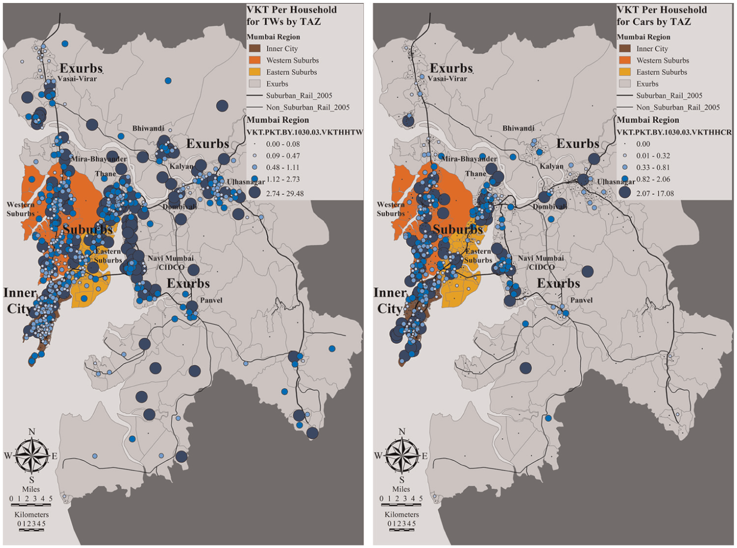
VKT per household for motorised two-wheelers (TWs) (left) and cars (right) in the Greater Mumbai Region (GMR); shown at home TAZ, where large circles show top quintile.

India has seen a mushrooming of private vehicle fleets since the mid 1990s. According to automobile industry figures, average annual sales of motorised two-wheelers (TWs) including motorcycles, scooters and mopeds grew by 12% between 2009 and 2015, while those of cars grew by 7% annually (Society of Indian Automobile Manufacturers, 2015). TWs with 50–350 cc engines are found commonly in South and Southeast Asia, yet the TW is an understudied mode (Dissanayake and Morikawa, 2010; Srinivasan et al., 2007; Yagi et al., 2013) – a gap this paper addresses. Especially, the impact of built environment variables on TW (and car) use is investigated here. This paper uses a cross-sectional data set from Mumbai to investigate how private vehicle use and built environment factors including density, diversity, job accessibility and transit access are linked, controlling for socio-economics. The hypothesis tested is that as households locate farther away from a city centre, all else being equal, their use of motorcycles, scooters and cars increases.

Literature review

The ‘Ds’ and built environment’s impact on vehicle use

Many factors influence vehicle use including built environment variables (Ewing and Cervero, 2010), complex trip chaining resulting from busy lifestyles (Schwanen and Lucas, 2011) and residential location choices (Houston et al., 2015). Overall, using the ‘Ds’ framework to study travel behaviour at a disaggregate level is informative. These numerous D factors, namely, density, diversity, design, destination accessibility and distance to transit have varying impacts on vehicle use.

Density’s influence on vehicle utility has received extensive treatment in transportation scholarship, but available evidence suggests that its impact is limited. Multiple studies find that density is negatively correlated with vehicle use (Cervero and Murakami, 2010; Chatman, 2009; Ewing et al., 2014). However, scholars also point out that higher density curbs vehicle use marginally, suggesting that it is an ineffective policy leaver (Bento et al., 2005; Brownstone and Fang, 2014).

Constrained residential location choice and vehicle use

Scholarship on height restrictions and floor area ratios in Indian cities suggests that limits to densification lead to an expansion of urban boundaries, constrain housing supply and increase generalised costs of transportation (Bertaud and Brueckner, 2005; Brueckner and Sridhar, 2012; Nallathiga, 2005). Furthermore, not just housing but also manufacturing and service jobs are moving outside urban centres (Singh, 2010; Sridhar, 2010). In the short term, anti-densification policies may seem reasonable for reducing crowding and restraining demand on infrastructure. However, with growing populations the resulting urban housing shortage is likely to constrain residential location choice.

Housing choices can be informed by preference for a specific travel mode such as transit (Houston et al., 2015) as well as other factors such as a preference for open space or wanting to live with one’s social class. Research suggests that households that make the choice of living close to transit have lower private vehicle use (Cervero, 2007; Ewing and Hamidi, 2014). More broadly, some researchers contend that self-selection impacts built environment estimates (Cao et al., 2009) while others argue that the impact of self-selection is unclear (Chatman, 2009).

Generally, in North America, households self-selecting to live in the suburbs have higher car use than those households self-selecting to live in city centres (Zhou and Kockelman, 2008). In comparison, Mumbai households, on average, have more car use in the city and higher TW use in the peripheries (Figure 1). In many cities, it is possible that those who live close to transit hubs derive benefits from the agglomerating jobs, shops and recreation. Such households likely have higher incomes, and own/use vehicles more (Bhat and Guo, 2007; Guerra, 2015). In contrast, those households that are priced out of locations near transit hubs and ‘choose’ to live farther out may need to use private vehicles to access transit or other opportunity sites for jobs and shopping. Thus, inadequate location choice in a constrained housing market may result in more vehicle use for those living farther from transit. To be conservatively cautious, in this research selection bias is computed and used as a covariate (see section ‘Bias correction measures’).

Background

Most often Mumbai is understood only as Mumbai City, but it has a large periphery. Inner City, the traditional employment centre, is located at the southern end of the peninsula (Figure 1). Inner City, along with the Western and Eastern Suburbs, falls under the Brihanmumbai Municipal Corporation. The region outside Mumbai City is a wide area with diffused urban agglomerations that are governed by various local bodies. These exurbs are made up of bedroom communities along with some nodes of industry and employment. The Greater Mumbai Region (GMR) is comprised of Mumbai City plus the exurbs, and the Mumbai Metropolitan Region Development Authority (MMRDA) is the metropolitan planning organisation for this region.

The GMR grew from 14.5 million in 1991 to 23.5 million in 2011. Mumbai City had 67% of the GMR’s population in 1991, yet this number shrunk to 53% in 2011 (Bhagat and Jones, 2013; LEA International Limited et al., 2008). Hence, the GMR has grown in population, but it is expanding outside Mumbai City. According to the 2011 Census, Mumbai City had a 20,700 persons/km² overall density, while the Region had a 5400 persons/km² gross density. Thus, Mumbai City still remains dominant in the region (Shirgaokar, 2014). Many major and minor nodes are spread across the GMR, yet Nariman Point in the Inner City remains a primary destination for employment (Shirgaokar, 2014: 253–255).

Expanding cities and housing supply

The outward growth of Indian cities has been happening for some time now, and has followed a particular trajectory. In the 1970s policymakers in India encouraged the de-congesting of cities, replicating practice from the developed world. With the view of encouraging new growth outside the congested urban centres, incentives such as higher floor area ratios were put into many municipal building codes for outer locations, while constraining density to equivalent levels in city centres. In Mumbai, in the 1970s policymakers encouraged the creation of secondary employment nodes such as Bandra Kurla Complex and urban periphery cities such as Navi Mumbai for housing. This kind of public-sector housing supply is a small part of current urban development policies. Today, private-sector housing is relatively plentiful and cheap in the peripheries, where the middle half of the income ladder comprised of the working poor and the emergent middle-class is moving. In the GMR, there is some evidence that not only housing but jobs too are moving out (LEA International Limited et al., 2008).

Transportation infrastructure and mode choice

On its website, MMRDA has a list of principal projects undertaken (MMRDA, 2015). Concentrating on the built transportation projects, a major focus on rail-based infrastructure is evident, with some spending on roads and rubber-based transit. For example, Metroline 1 connecting the Eastern and Western suburbs between Ghatkopar and Versova opened in 2014; an elevated system, this cost ₹ 23.6 billion (US$ 0.37 billion). Similarly, a monorail line went into operation in 2014 connecting the Eastern and Western Suburbs between Chembur and Wadala; the project cost was ₹ 24.6 billion (US$ 0.38 billion). The Maharashtra State Road Development Corporation Limited built an eight-lane cable-stayed bridge between Bandra and Worli at ₹ 16.3 billion (US$ 0.25 billion) (Phadke, 2014). Though these investments are needed, generally there has been more capital spending for infrastructure supply within Mumbai City and marginal investment outside (Phadke, 2013).

Some transportation investments are made with the aim of linking Mumbai City with the rest of the GMR, or with the intention of opening up new areas for development. Public–private enterprises supply buses that enable trips between exurban agglomerations and major employment centres or transit nodes. These travel options do provide choices to passengers between multiple points along arterials. Yet those who live away from the infrastructure corridors face the first-mile problem, which is solved sometimes by using a rickshaw or jitney service. In locations with weak supply of these options, working poor and emergent middle class households often walk or bicycle. Some individuals might elect to use TWs and cars, depending on the distance they need to travel and their money value of time.

Data

The cross-sectional data used for this paper are from a household travel survey conducted in the GMR by the MMRDA between April 2005 and April 2006. Overall, this data set comprises a random 1.5% sample of the total population (about 66,000 households) within the GMR (LEA International Limited et al., 2008). For the purpose of this analysis, private mode trips are all unlinked trips that were reported in the travel diary undertaken by a motorised two-wheeler (TW) or car driver. Generally, TWs include all classes of motorised two-wheelers including motorcycles, scooters and mopeds. Cars include all classes of motorised four-wheelers including sedans, coupes, jeeps, mini-vans and sports utility vehicles. Of the 182,600 trips that middle class households made on an average weekday, 11,200 trips (6%) were made using a two-wheeler or car where the trip-maker was a driver. About 19% of these total private mode trips were non-work related, but were for school, shopping, recreation, etc. For this analysis, all trip purposes are included since the research focuses on total household vehicle use.

Geography of private vehicle use in Mumbai

Figure 1 shows the spatial nature of private vehicle use in the GMR reported as vehicle kilometres travelled (VKT) in a household at the Traffic Analysis Zone (TAZ) level. Focusing only on the top quintile, shown by large circles, it is evident that the highest car use is concentrated in Mumbai City along the transportation corridors (right image), and in secondary cities such as Thane and Navi Mumbai. However, TW use is much more ubiquitous and shows up in all urban agglomerations, particularly in the exurbs (left image).

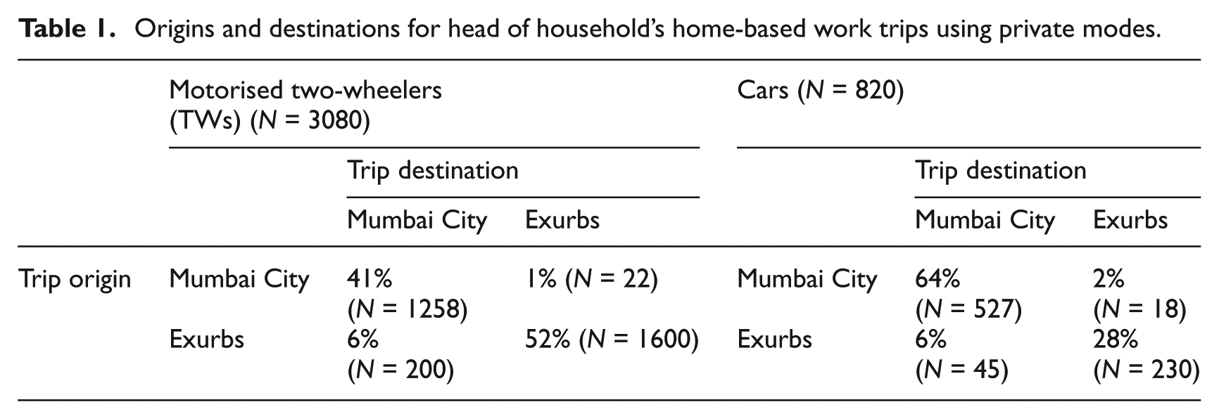
Aggregate origin-destination tabulation (Table 1) lends further support to the idea that TWs are used outside Mumbai city. Specifically, 52% of the trips from home to work by the head of household using a TW begin and end in exurbs, while car trips are concentrated within Mumbai City with 64% of these trips beginning and ending within Mumbai City.

Table 1.

Origins and destinations for head of household’s home-based work trips using private modes.

	Motorised two-wheelers (TWs) (N = 3080)			Cars (N = 820)
		Trip destination			Trip destination
		Mumbai City	Exurbs		Mumbai City	Exurbs
Trip origin	Mumbai City	41% (N = 1258)	1% (N = 22)	Mumbai City	64% (N = 527)	2% (N = 18)
Trip origin	Exurbs	6% (N = 200)	52% (N = 1600)	Exurbs	6% (N = 45)	28% (N = 230)

Variables used in the analysis

An overview of variables used in this analysis is presented in Table 2, followed by a discussion regarding the construction of covariates. Many of the variables entered the models in their natural log form, but are reported in their original form. The variables are reported in four groups in Table 2, namely households where VKT was either greater than zero or zero, for TWs and cars. Some key observations are:

Households reporting car access, especially those reporting use, tend to live closer to Nariman Point, the principal financial centre of Mumbai suggesting a residential location bias.

Accessibility to jobs by cars is lower in comparison to TWs indicating that low speeds for car travel impact destination accessibility.

A comparison of the density metrics suggests that, on average, car users live and work in denser places, while TW users live and work in locations with lower density.

As expected, per capita annual household income is highest for the households that use cars and lowest in the group where TW use is zero.

Two-thirds of the heads of households in the car use group have a college education (or a technical diploma), while an almost equal number in the TW use group do not.

Variables for total persons, adults and the presence of a child in the household suggest that bigger household size may negatively affect vehicle use.

Table 2.

Overview of variables used.

Variable description	Variable name^a	VKT TW (non-zero) (N = 3133)		VKT TW = 0 (N = 2764)		VKT CAR (non-zero) (N = 842)		VKT CAR = 0 (N = 1044)
		Mean (mode)	Std. dev.^b	Mean (mode)	Std. dev.^b	Mean (mode)	Std. dev.^b	Mean (mode)	Std. dev.^b
Vehicle kilometres travelled (VKT) by all members of a household (private mode trips only, all trip purposes) (km)	VKTTWHHPLUS1LN or VKTCARHHPLUS1LN	13.9	15.6	–	–	19.0	18.5	–	–
Location
Street network distance from centroid of home TAZ to the principal employment centre, Nariman Point (km)	ODISTNMPTNREDLN	37.4	20.3	39.3	19.6	26.7	17.5	33.6	19.8
Head of household’s usual place of work (1 = Inner City, 0 = Other)	WKISMUMDM	(0)	84%	(0)	74%	(0)	68%	(0)	69%
Land use
Job accessibility by motorised two-wheeler (‘000)	HHTZAI076TWTTLEMPLFN	853	682	804	686
Job accessibility by car (‘000)	HHTZAI082CARTTLEMPLFN					795	539	771	578
Home TAZ land use diversity	HHTZDI	0.48	0.15	0.48	0.15	0.50	0.15	0.49	0.15
Population density at home TAZ (persons/km²) (‘000)	HHTZPOPDENCRSLN	617	1186	624	1253
Housing density at home TAZ (residences/km²) (‘000)	HHPRKM2LN					12.3	19.1	11.2	15.3
Employment density at head of household’s work TAZ (employees/km²) (‘000)	UPETZTTLEMPLDENCRSLN	263	458	289	488	349	465	295	421
Infrastructure supply
Network distance to nearest railway station from centroid of home TAZ	HHNTDISTSTATLN	2.6	3.1	2.6	3.2
Centroid of home TAZ within straight-line distance of 250 m from a railway station (yes = 1, no = 0)	HHEUDISTSTAT250MTDM					(0)	97%	(0)	96%
Street density at home TAZ (street length/km²)^c	HHTZSTREETDENPLUS1LN	3.9	3.3	4.0	3.3
Socio-economics
Per capita annual household income in Indian Rupees ₹ (’000)	PRCPTHHINCLN	41	26	39	25	69	44	51	38
Head of household has a technical diploma or is college educated (yes = 1, no = 0)	EDUCDM	(0)	69%	(0)	66%	(1)	66%	(1)	51%
Total private parking per household^c,d	TTLPRIVPKPLUS1LN	1.2	0.5	1.1	0.5
Type of residence is apartment or independent house (yes = 1, no = 0)	RESTYPDM					(1)	90%	(1)	83%
Total persons in the household	TOTALPERSONSLN	3.0	1.2	3.1	1.3
Total adults in the household	TOTALADULTSLN					2.2	1.1	2.3	1.1
Children dummy (yes = 1, no = 0)	CHILDHHDM					(0)	61%	(0)	53%
Motorised two-wheelers available per total persons in the household	TWAVILPERTTLPRSNS	0.4	0.2	0.4	0.2
Cars available per total persons in the household	CARAVILPERTTLPRSNS					0.5	0.3	0.4	0.3
Bias correction measures (see section ‘Bias correction measures’)
Expected number of vehicles	ENV	0.3	0.2	0.3	0.2	0.4	0.2	0.4	0.2
Self-selection bias correction	SBC	−1.5	0.4	−1.5	0.4	−1.2	0.1	−1.2	0.2

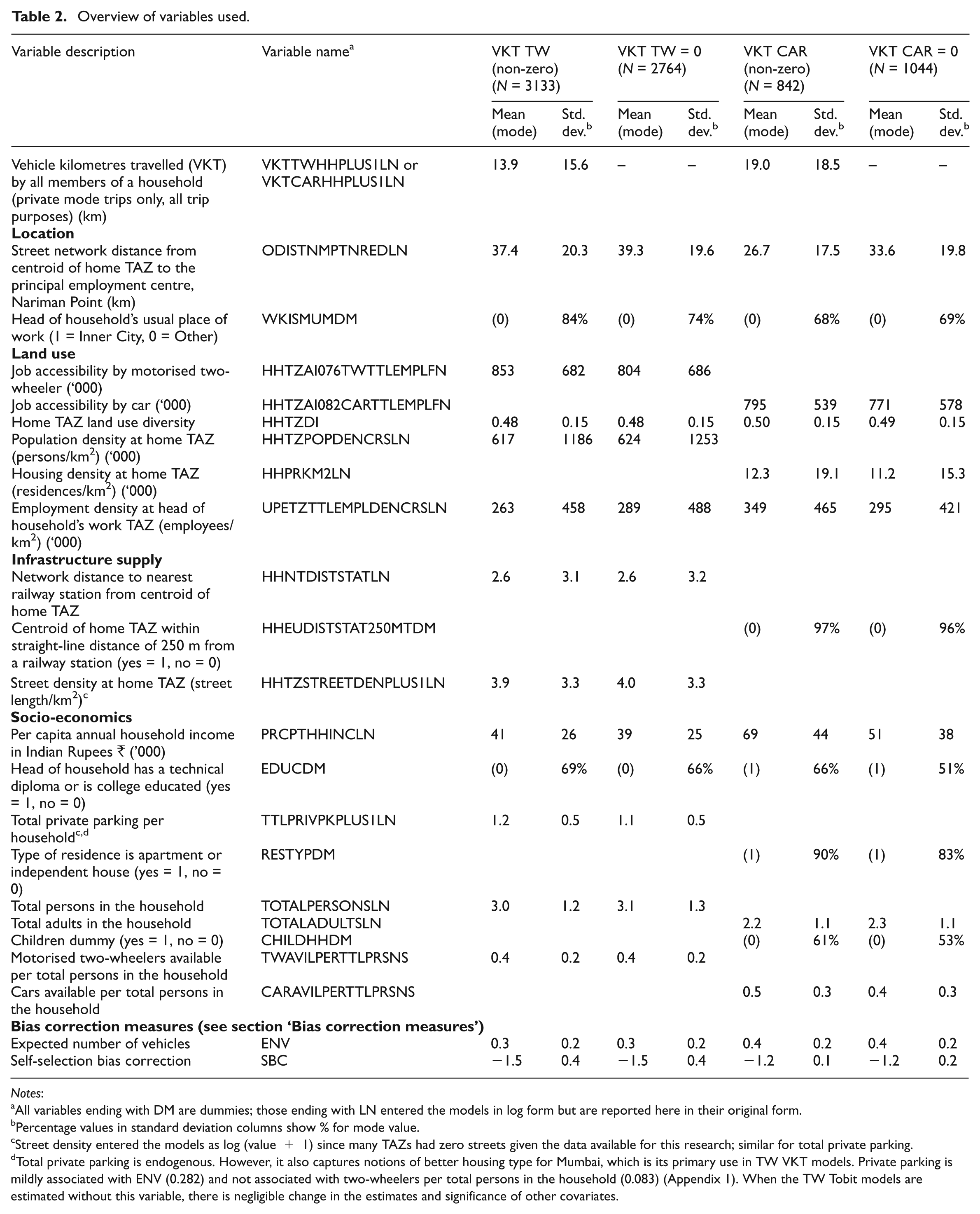
Notes:

All variables ending with DM are dummies; those ending with LN entered the models in log form but are reported here in their original form.

Percentage values in standard deviation columns show % for mode value.

Street density entered the models as log (value + 1) since many TAZs had zero streets given the data available for this research; similar for total private parking.

Total private parking is endogenous. However, it also captures notions of better housing type for Mumbai, which is its primary use in TW VKT models. Private parking is mildly associated with ENV (0.282) and not associated with two-wheelers per total persons in the household (0.083) (Appendix 1). When the TW Tobit models are estimated without this variable, there is negligible change in the estimates and significance of other covariates.

Vehicles kilometres travelled by household

Any household that reported access, i.e. ownership or availability, to a TW or car was included in this analysis. Of all the middle class households surveyed only 5897 (9%) households had access to at least one TW, and just 1886 (3%) households had access to at least one car. Not all middle class households that had such access reported using the vehicle on the survey day; merely 3133 (53%) households with access to TW and 842 (45%) households with access to cars generated some VKT.

To construct the dependent variable vehicle kilometres travelled (VKT) per household, these private mode trips were aggregated by TW and car at the household level. It was not possible to compute exact trip lengths since the available street network did not have sufficient detail, so trips lengths were computed between TAZ centroids. Lengths for all trips that started and ended in the same TAZ were calculated as radius of a circle of area equal to that TAZ. Since some of the private vehicle trip lengths were imputed from TAZ areas, a few households had rather small VKT, i.e. less than 0.25 km per day. Only those households whose total vehicle use on the survey day was more than 0.25 km were identified as having valid VKT (section ‘Model specifications’).

Location measures

To study impacts of location on vehicle use, two variables – household distance from city centre (Zegras, 2010) and usual place of work for head of household – were used. Distance along the street network between the home location’s TAZ centroid and Nariman point, as the primary employment node, was computed in kilometres. Workplace location for head of household in Inner City (Figure 1) was a dummy variable.

Land use measures

A destination accessibility indicator measures the number of opportunity sites (e.g. jobs) accessible from a location (household TAZ) by a travel mode (TW or car) weighed by the negative exponent of travel time. This measure was calculated for each TAZ by both travel modes and assigned to the household according to its home location TAZ. The value was computed using the equation (Guerra, 2014):

A_{i, m} = \sum_{i = 1}^{j} J_{j} * e^{(- d_{m} * T T_{ij, m})}

(1)

where, A_i,m is job accessibility in TAZ i by mode m, travel mode m is TW or car, J is number of jobs in TAZ j (available from MMRDA), d_m is impedance factor calculated as one over the regional average commute distance by travel mode m (Hu, 2014), and TT is mode-specific travel time in minutes between centroids of TAZs i and j for TW and car trips. The regional average commute distance for TW was 13.1 km, giving an impedance factor of 0.076, while that for car was 12.2 km, giving an impedance factor of 0.082.

Typically land use diversity is an indicator showing how much variety in land uses exists in an area, computed based on the square metres of various use categories such as housing, office, retail, etc. (Rajamani et al., 2003; Zegras, 2010). Since detailed land use data were not available for this analysis, the diversity index was computed using trip destination and trip purpose (Guerra, 2014). The index was computed for each TAZ using four trip purposes, namely, housing, work, school and other, and then assigned to each household based on its reported TAZ. This measure was computed using the formula:

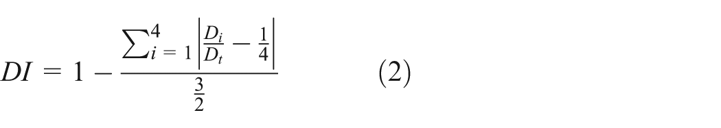
DI = 1 - \frac{\sum_{i = 1}^{4} | \frac{D_{i}}{D_{t}} - \frac{1}{4} |}{\frac{3}{2}}

(2)

where, DI is diversity index in a given TAZ, D_i is number of trip destinations in the TAZ in each category, home, work, school and other, and D_t is total trip destinations in the TAZ.

Three measures of density were used in the two mode-specific models (Table 2). Each density metric was calculated using the numbers from the strategic level of aggregation in MMRDA’s TAZ system, divided by the corresponding area. Under MMRDA’s TAZ system 1030 TAZs were grouped into 171 strategic zones. These coarse measures were calculated on purpose to reduce the impact of high-density nodes. Population density factored in number of people, housing density relied on number of housing units, and employment density had the number of employees at the head of a household’s workplace.

Infrastructure supply measures

Some measures were used to capture the impact of available transportation infrastructure on vehicle use. These covariates were distance to the nearest rail station and street density. Proximity to transit was captured using two variables, one using street distance and another as a dummy. However, the focus was only on railway stations since there were no data available on bus, rickshaws, taxis and other forms of jitney services. Since data on the availability of all other modes were not included in this measure on transit supply, the coefficients computed likely underestimate the effect.

Street density was computed at home TAZ as length of all classes of streets in the TAZ divided by TAZ area in square kilometres (Li et al., 2010). However, the street network was not detailed and likely did not include minor streets and alleys. Therefore, this metric also likely underestimates the impact of street supply on vehicle use.

Socio-economic measures

A few different socio-economic measures were used in the VKT models for TW and car use such as per capita annual household income and a dummy for higher education for the head of household. Total private parking in the household (Table 2, footnote d) was used in the TW VKT models as an alternative for the type of residence dummy used in car use models.

Other socio-economic measures included total persons and total adults in the household; the latter measure does not include children younger than 16 years. This age cut-off is used since only at 16 years is it possible to get a driving license for low-powered TWs in India. A dummy for children under 16 was also set up for the car VKT models, enabling full information on household composition to be expressed in the car use models.

To test if changing the expected number of vehicle variable altered the estimates, TWs (or cars) available per total persons was used (sections ‘Bias correction measures’ and ‘Limitations’).

Bias correction measures

Two measures were calculated to correct for endogeneity and selection bias (Houston et al., 2015; Zegras, 2010). The expectation of a vehicle in the household, as an exogenous and independent variable, was calculated based on an estimated multinomial logit (MNL) model on vehicle ownership (not reported here). The formula used to calculate ENV was:

EN V_{l, m} = 0 * P_{l, 0, m} + 1 * P_{l, 1, m}

(3)

where, ENV_l,m is expected number of private vehicles for household l by mode m, m is TW or car, P_l,k,m is predicted probability of household l having access to a TW or car, where k can equal 0 or 1.

A second measure to counter self-selection (section ‘Constrained residential location choice and vehicle use) was constructed as a correction. SBC was calculated using the equation:

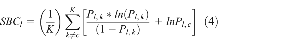
SB C_{l} = (\frac{1}{K}) \sum_{k \neq c}^{K} [\frac{P_{l, k} * \ln (P_{l, k})}{(1 - P_{l, k})} + \ln P_{l, c}]

(4)

where, SBC_l is self-selection correction for household l, K is total number of alternatives, k is alternative index (0 or 1 private vehicle), c is chosen alternative index, P_l,k is predicted probability of household l owing k vehicles (from MNL).

Model specifications

Three model specifications were used to tease out the impacts of built environment and socio-economic variables on vehicle use: a binary logit form of log odds to study non-zero VKT households, a Tobit model to correct for left censoring of the dependent variable, and a censored quantile regression to figure out the impacts of the covariates on different levels of vehicle use.

Many of the households who had access to a TW or car chose not to use it on the survey day (section ‘Vehicles kilometres travelled by household’). The likelihood that a household had non-zero VKT was modelled using a binary logit form (Ewing et al., 2015). The following system of equations expresses the binary logit model (Long, 1997):

y_{l, m} = {\begin{matrix} 1, if VK T_{l, m} > 0.25 \\ 0, if VK T_{l, m} \leq 0.25 \end{matrix}

(5)

P_{l, m} (1) = P (U_{l, m, 1} \geq U_{l, m, 0})

(6)

U_{l, m} = V_{l, m} + ε_{l, m}

(7)

P_{l, m} (1) = \frac{e^{V_{l, m, 1}}}{e^{V_{l, m, 1}} + e^{V_{l, m, 0}}}

(8)

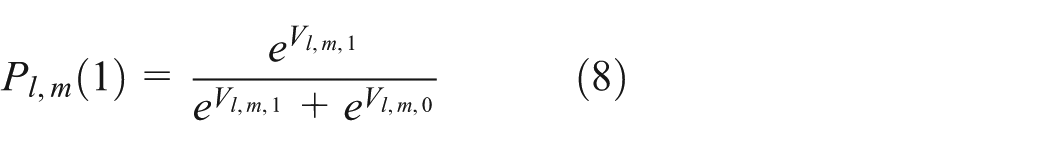
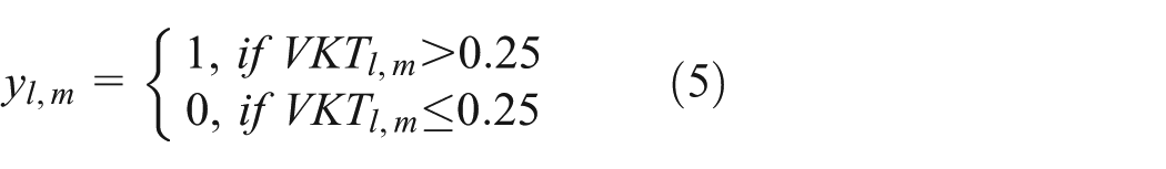
where, y is binary dependent variable, l is index of household, m is mode (TW or car), $P_{l, m} (1)$ is probability that household l using mode m had VKT > 0.25 km, $U_{l, m, k}$ is a utility expression for household l using mode m (k = 1 or 0), $V_{l, m}$ is systematic component of utility expression for household l using mode m, and $ε_{l, m}$ is a random component of utility expression for household l using mode m.

Household VKT can be modelled using a log-log ordinary least squares specification. However, the likelihood of getting biased estimates is high since the dependent variable VKT for both modes theoretically stops at zero, and has a long-tailed positive distribution. Hence, a Tobit regression form for such a left-censored distribution was chosen (Chatman, 2003; Houston et al., 2015). However, the cut-off was set to 0.25 km rather than 0 km of VKT in the household (section ‘Vehicles kilometres travelled by household’). The dependent variable was transformed to the natural log of (1 plus VKT) (Guerra, 2014). The Tobit model specification takes the following form (Long, 1997):

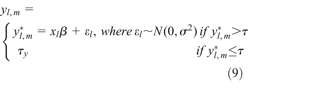
y_{l, m} = {\begin{matrix} y_{l, m}^{*} = x_{l} β + ε_{l}, & w h e r e ε_{l} ~ N (0, σ^{2}) i f y_{l, m}^{*} > τ \\ τ_{y} & i f y_{l, m}^{*} \leq τ \end{matrix}

(9)

where, $y_{l, m}$ is dependent variable VKT for household l and mode m, $x_{l}$ stands for covariates for household l, $ε_{l}$ is an error term for household l, and $τ$ is VKT at 0.25 km.

Another question of interest was how the amount of driving by TW or car in a household, at the 25th, 50th and 75th use quantiles, was connected to the built environment and socio-economic variables. These models were run as censored regressions using the ‘quantreg’ package, crq fitting function and por censored quantile regression estimator in R (Koenker, 2008; Portnoy, 2003).

Model results

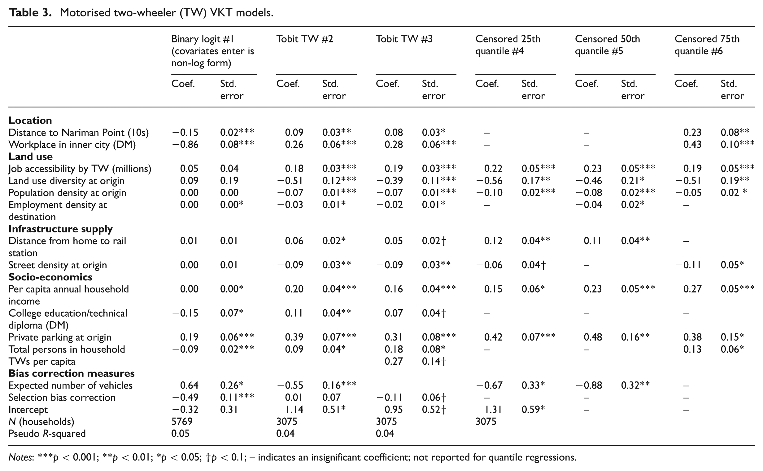
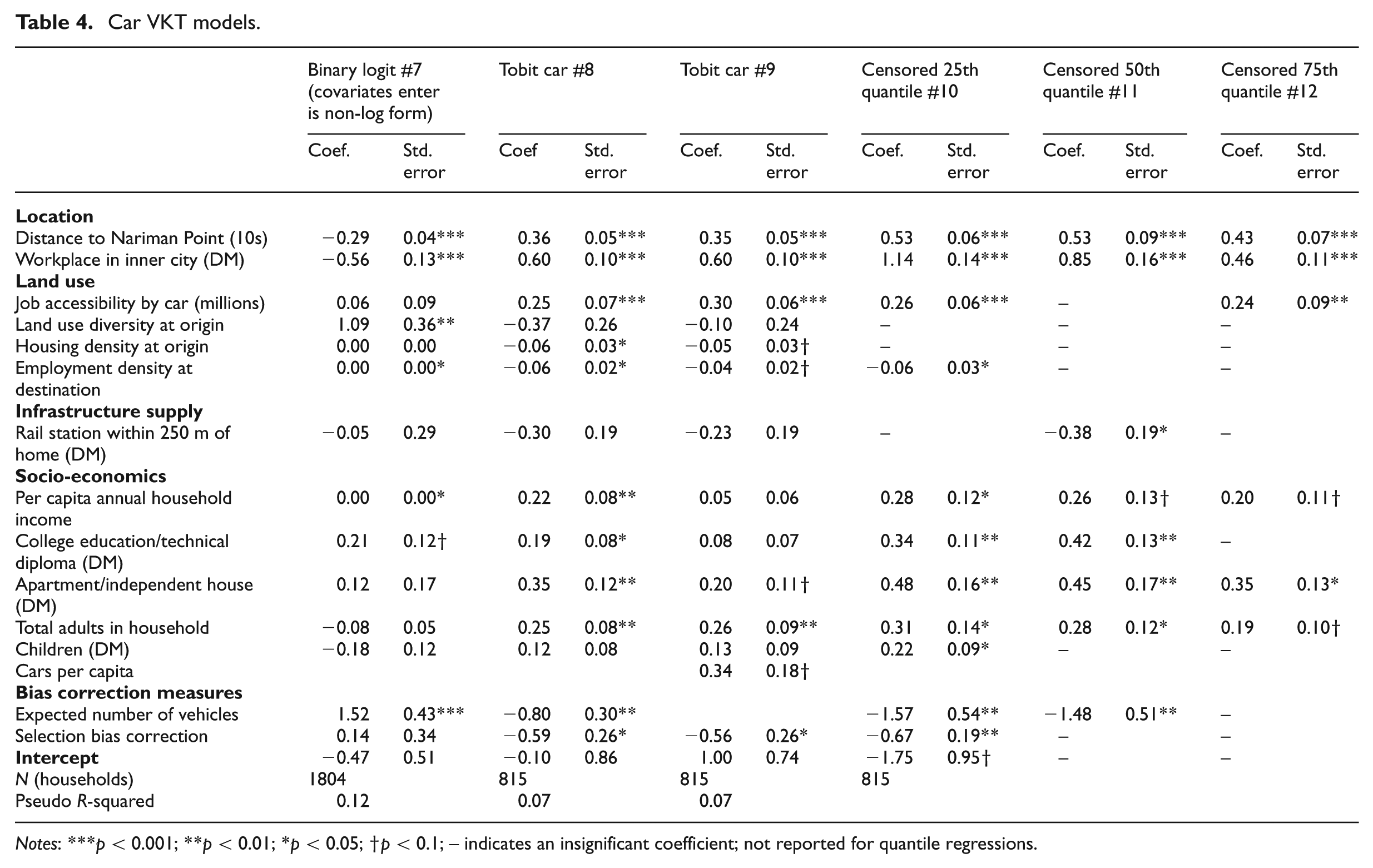
In this section, Tables 3 and 4 show findings from the models for TWs and cars, respectively. Note that the binary logit models did not have log transformed covariates for continuous variables entering the model estimation. The Tobit models were run with ENV (equation 3) as well as with the alternative variables, per capita TW (or car) ownership.

Table 3.

Motorised two-wheeler (TW) VKT models.

	Binary logit #1 (covariates enter is non-log form)		Tobit TW #2		Tobit TW #3		Censored 25th quantile #4		Censored 50th quantile #5		Censored 75th quantile #6
	Coef.	Std. error	Coef.	Std. error	Coef.	Std. error	Coef.	Std. error	Coef.	Std. error	Coef.	Std. error
Location
Distance to Nariman Point (10s)	−0.15	0.02***	0.09	0.03**	0.08	0.03*	–		–		0.23	0.08**
Workplace in inner city (DM)	−0.86	0.08***	0.26	0.06***	0.28	0.06***	–		–		0.43	0.10***
Land use
Job accessibility by TW (millions)	0.05	0.04	0.18	0.03***	0.19	0.03***	0.22	0.05***	0.23	0.05***	0.19	0.05***
Land use diversity at origin	0.09	0.19	−0.51	0.12***	−0.39	0.11***	−0.56	0.17**	−0.46	0.21*	−0.51	0.19**
Population density at origin	0.00	0.00	−0.07	0.01***	−0.07	0.01***	−0.10	0.02***	−0.08	0.02***	−0.05	0.02 *
Employment density at destination	0.00	0.00*	−0.03	0.01*	−0.02	0.01*	–		−0.04	0.02*	–
Infrastructure supply
Distance from home to rail station	0.01	0.01	0.06	0.02*	0.05	0.02†	0.12	0.04**	0.11	0.04**	–
Street density at origin	0.00	0.01	−0.09	0.03**	−0.09	0.03**	−0.06	0.04†	–		−0.11	0.05*
Socio-economics
Per capita annual household income	0.00	0.00*	0.20	0.04***	0.16	0.04***	0.15	0.06*	0.23	0.05***	0.27	0.05***
College education/technical diploma (DM)	−0.15	0.07*	0.11	0.04**	0.07	0.04†	–		–		–
Private parking at origin	0.19	0.06***	0.39	0.07***	0.31	0.08***	0.42	0.07***	0.48	0.16**	0.38	0.15*
Total persons in household	−0.09	0.02***	0.09	0.04*	0.18	0.08*	–		–		0.13	0.06*
TWs per capita					0.27	0.14†
Bias correction measures
Expected number of vehicles	0.64	0.26*	−0.55	0.16***			−0.67	0.33*	−0.88	0.32**	–
Selection bias correction	−0.49	0.11***	0.01	0.07	−0.11	0.06†	–		–		–
Intercept	−0.32	0.31	1.14	0.51*	0.95	0.52†	1.31	0.59*	–		–
N (households)	5769		3075		3075		3075
Pseudo R-squared	0.05		0.04		0.04

Notes: ***p < 0.001; **p < 0.01; *p < 0.05; †p < 0.1; – indicates an insignificant coefficient; not reported for quantile regressions.

Table 4.

Car VKT models.

	Binary logit #7 (covariates enter is non-log form)		Tobit car #8		Tobit car #9		Censored 25th quantile #10		Censored 50th quantile #11		Censored 75th quantile #12
	Coef.	Std. error	Coef	Std. error	Coef.	Std. error	Coef.	Std. error	Coef.	Std. error	Coef.	Std. error
Location
Distance to Nariman Point (10s)	−0.29	0.04***	0.36	0.05***	0.35	0.05***	0.53	0.06***	0.53	0.09***	0.43	0.07***
Workplace in inner city (DM)	−0.56	0.13***	0.60	0.10***	0.60	0.10***	1.14	0.14***	0.85	0.16***	0.46	0.11***
Land use
Job accessibility by car (millions)	0.06	0.09	0.25	0.07***	0.30	0.06***	0.26	0.06***	–		0.24	0.09**
Land use diversity at origin	1.09	0.36**	−0.37	0.26	−0.10	0.24	–		–		–
Housing density at origin	0.00	0.00	−0.06	0.03*	−0.05	0.03†	–		–		–
Employment density at destination	0.00	0.00*	−0.06	0.02*	−0.04	0.02†	−0.06	0.03*	–		–
Infrastructure supply
Rail station within 250 m of home (DM)	−0.05	0.29	−0.30	0.19	−0.23	0.19	–		−0.38	0.19*	–
Socio-economics
Per capita annual household income	0.00	0.00*	0.22	0.08**	0.05	0.06	0.28	0.12*	0.26	0.13†	0.20	0.11†
College education/technical diploma (DM)	0.21	0.12†	0.19	0.08*	0.08	0.07	0.34	0.11**	0.42	0.13**	–
Apartment/independent house (DM)	0.12	0.17	0.35	0.12**	0.20	0.11†	0.48	0.16**	0.45	0.17**	0.35	0.13*
Total adults in household	−0.08	0.05	0.25	0.08**	0.26	0.09**	0.31	0.14*	0.28	0.12*	0.19	0.10†
Children (DM)	−0.18	0.12	0.12	0.08	0.13	0.09	0.22	0.09*	–		–
Cars per capita					0.34	0.18†
Bias correction measures
Expected number of vehicles	1.52	0.43***	−0.80	0.30**			−1.57	0.54**	−1.48	0.51**	–
Selection bias correction	0.14	0.34	−0.59	0.26*	−0.56	0.26*	−0.67	0.19**	–		–
Intercept	−0.47	0.51	−0.10	0.86	1.00	0.74	−1.75	0.95†	–		–
N (households)	1804		815		815		815
Pseudo R-squared	0.12		0.07		0.07

Notes: ***p < 0.001; **p < 0.01; *p < 0.05; †p < 0.1; – indicates an insignificant coefficient; not reported for quantile regressions.

TW use models

Table 3 shows that the land use, infrastructure supply and socio-economic variables are largely significant for the Tobit and censored quantile models. The location variable coefficients support the hypothesis that the farther a household is located from Nariman Point, TW use increases, all else being equal. Specifically, a 10-km increase in distance of the household from Nariman Point increases TW VKT by 9% (model #2, log-log form). For households who use their TWs a lot (model #6), this change in location results in a 23% increase in TW use. Jobs are distributed across the GMR but if the head of household shifts to working in the Inner City (Figure 1), TW VKT goes up by 30% (#2, $e^{0.26}$ = 1.30); at the 75th quantile, TW use goes up by 54% (#6, $e^{0.43}$ = 1.54). The binary logit shows that a 10-km increase in household location from Nariman Point, will reduce the odds of a household going from no use to the vehicle use group by 14% (#1, $e^{- 0.15}$ = 0.86), holding all else constant. If the head of household started working in the Inner City, the probability of the household going from no use to TW use decreases by 58% (#1, $e^{- 0.86}$ = 0.42).

A 1-unit increase in accessibility to jobs (equation 1) results in a 20% increase in TW VKT (#2, $e^{0.18}$ = 1.20). As expected, increasing land use diversity brings down TW VKT. A 1-unit increase in land use diversity (equation 2) results in 40% decrease in TW use (#2, $e^{- 0.51}$ = 0.60). This large impact that land use diversity has in bringing down TW use is notable. In contrast, increasing density has a marginal effect on reducing TW use. A 10% increase in population density at the home location results in a 0.7% downward shift in TW use (#2, log-log form), and a 10% increase in employment density at the head of household’s work place decreases TW VKT by 0.3%.

A 10% increase in the distance between the home and railway station would result in a 0.6% increase in TW VKT (#2, log-log form). A counter-intuitive finding is that supplying more road space brings down TW VKT. Specifically, a 10% increase in street density decreases TW VKT by 0.9% (#2, log-log form). A possibly explanation is that this covariate is capturing some impacts of street congestion.

Within the socio-economic variables, a 10% growth in per capita income increases TW VKT by 2% (#2, log-log form). Better education similarly increases TW use, with the head of household having a college education resulting in a 12% increase in TW use (#2, $e^{0.11}$ = 1.12). If household size increases by 10%, TW VKT grows by 9% (#2, log-log form).

Higher ENV (equation 3) is linked to lower TW use; specifically the expectation of a TW in a household reduces its use by 42% (#2, $e^{- 0.55}$ = 0.58), all else being equal (section ‘Limitations’). A reduced model with just ENV as an explanatory variable results in a positive TW VKT (not shown here, $e^{0.20}$ = 1.22). Further, the binary logit (#1, $e^{0.64}$ = 1.90) suggests that odds of TW use increase with expectation of a TW, and using TWs per capita (#3, $e^{0.27}$ = 1.30) shows increasing TW use.

Car use models

The car VKT models (Table 4) suggest that location and socio-economics have a greater impact on car use than land use and infrastructure supply. Location variables support the hypothesis that increasing distance of household location from Nariman Point is linked to higher car use, holding all else equal. This effect is much stronger for car use than TW use; specifically a 10-km increase in distance of home location from Nariman Point increases car use by 36% (model #8, log-log form). If the head of household makes the change to work in the Inner City (Figure 1), car use increases dramatically by 83% (#8, $e^{0.60}$ = 1.83). The binary logit (#7) estimates suggest that moving the home location 10-km away from Nariman Point, brings down the likelihood of moving from the nonuse to car use group by 25% (#7, $e^{- 0.29}$ = 0.75). Also, if the head of household starts working at Nariman Point, the odds of the household using a car drop by 43% (#7, $e^{- 0.56}$ = 0.57).

Land use and infrastructure supply measures have less predictive power for car use than TW use, indicating that car use is not strongly impacted by these factors. Yet there are a few significant findings, for example, better job accessibility by car increases car VKT, and the impacts are larger than those for TWs. Specifically, a 1-unit increase in accessibility to jobs by car (equation 1) results in a 29% increase in car VKT (#8, $e^{0.25}$ = 1.29). Higher density has a marginal impact on car use, similar to TW use. Increasing housing density by 10% results in a 0.6% decline in car use (#8, log-log form), and an equal impact is predicted from increasing employment density by 10%.

Overall, socio-economic variables have a greater impact on car use than TW use, though the effect of a 10% increase in per capita income is similar between the two modes, i.e. a 2% increase in car VKT (#8, log-log form). If the head of household has a college education (or technical diploma), car VKT increases by 21% (#8, $e^{0.19}$ = 1.21). At the 50th quantile of car use, the impact of college education is more pronounced at 52% (#11, $e^{0.42}$ = 1.52). Living in an apartment/independent house, predicts higher car use at 42% (#8, $e^{0.35}$ = 1.42). Car VKT also increases with more adults in the household; a 10% increase in adults in the household is linked to a 25% increase in car use (#8, log-log form).

A 1-unit increase in ENV (equation 3) decreases car use by 55% (#8, $e^{- 0.80}$ = 0.45). A reduced model with just ENV as an independent variable has a positive but insignificant coefficient. The odds of moving from the nonuse to car use group increases dramatically with a 1-unit increase in ENV for car (#7, $e^{1.52}$ = 4.59), and using cars per capita instead of ENV results in an increase of 40% in car use (#9, $e^{0.34}$ = 1.40). A 1-unit increase in SBC (equation 4) decreases car use by 45% (#8, $e^{- 0.59}$ = 0.55).

Limitations

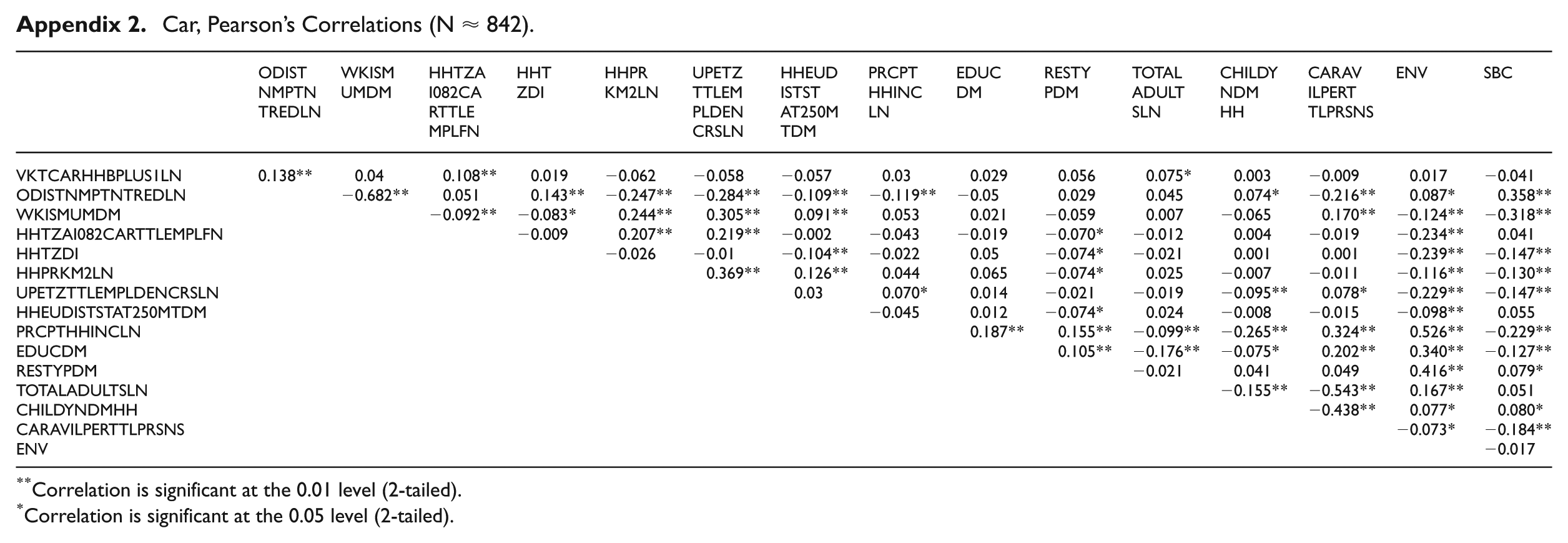
Of the random 66,000 households, just 11% had TW access and merely 3% had car access. When analysing ownership using a multinomial logit model (not reported here), expected probabilities of owning TWs or cars were negligible. Therefore, the expected number of vehicles (ENV) (equation 3) also computed as a small number for most households (Table 2). Appendices 1 and 2 present correlation matrices for variables entering the TW and car models respectively; and the correlation between VKT and ENV is weak for both private modes. ENV is used in the Tobit regressions as an instrument and exogenous variable, but its coefficient has a counter-intuitive sign. Running tests with reduced models shows that the impact of ENV is positive on vehicle use, as expected. The likely explanation for the negative coefficient is that the other explanatory variables take away the marginal impact of ENV on VKT. However, this finding needs further study since some alternative measures of vehicle access have positive estimates.

Housing self-selection presupposes that residential mobility exists; an assumption that is less likely to hold in the developing world. In India many households cannot afford to live in dense inner city environments given the constrained housing supply. Those with higher incomes, however, may live in such locations with transit supply, yet might choose to drive (Bhat and Guo, 2007; Salon et al., 2012). Though the research in this paper controls for self-selection (equation 4), joint modelling of travel and residential location may be better suited to understand how the two choices are interconnected.

Comparisons and conclusions

There is a growing body of research about Asia that examines travel behaviour. However, given limited data on land use and transportation networks, these studies have largely depended either on socio-economic variables to understand user preferences, or on small samples. These efforts offer important advances in thinking about travel behaviour in this region. A few published studies have delved into the built environment, where they use measures such as CBD versus non-CBD trips (Dissanayake and Morikawa, 2010), proximity to activity nodes (Srinivasan et al., 2007) and job density (Yagi et al., 2013). Some of these findings can be used to validate the outcomes of this current work on Mumbai. Ewing and Cervero (2010) offer a VKT-built environment meta-analysis, which is also appropriate given the limited number of studies about Asia using comparable covariates.

This paper, using disaggregate household travel survey data, reveals the connection between the built environment and vehicle use for motorised TWs such as motorcycles and scooters, and for cars in Mumbai. This study’s hypothesis, that the farther a household is located from a city centre the greater its use of TWs and cars, is supported in the literature (Srinivasan et al., 2007; Yagi et al., 2013; Zegras, 2010). The impact of distance from the city centre is higher for car use than TW use in Mumbai (Tables 3 and 4), suggesting that as Indian cities expand the use of cars may increase more than TWs.

As expected, most of the socio-economic variable estimates indicate that higher income, more education, better housing and bigger household size are associated with increasing TW use (Table 3, model #2). A counter-intuitive finding is that the impact of better education and bigger household size is negative on the odds of TW use in a household (Table 3, model #1). Thus, as education improves and if household sizes grow it is likely that TW use may go down for some families. However, whether the unmet travel demand shifts to transit or car use is a question for further research.

Greater income, college education, better housing and more adults in a household have a relatively strong impact on car use compared with TW use (Table 4, model #8). Overall, these findings suggest that TWs and cars act as substitutes rather than complements. A comparison between the model outcomes suggests that TW use is greater at lower education levels, but as socio-economics get better, car use goes up. It is likely that substitution occurs across a household’s life cycle, e.g. a household with just TWs in early married years shifts to a mixed fleet of TWs and cars over the years. Substitution can also occur within a household at a given time, e.g. the head of household uses the car for work trips but relies on a TW for quick errands around the neighborhood.

Elasticity estimates and validation

Mode-specific elasticities for this study are calculated first as marginal effects for each household and then averages are presented in Table 5 (Salon et al., 2012). Higher job accessibility by private modes increases VKT comparably for TWs and cars, though this impact is smaller than found in other studies (e.g. Guerra, 2014). This suggests that investments in the urban street network may increase VKT as private mode travel time improves (Shirgaokar, 2014: Appendix A). So policies that encourage investment in road space may induce higher private vehicle use. In contrast, street density elasticity suggests that TW use decreases at higher values of street length per square kilometre. This variable is likely capturing congestion effects and availability of other travel options such as rickshaws and shared cabs in locations with better street networks. The elasticity for proximity to rail transit suggests a marginal increase in TW use the further a household locates from a rail station. These values for street density and distance to a rail station are similar to findings in the meta-analysis (Ewing and Cervero, 2010: tables A-3 and A-5).

Table 5.

Elasticities (computed by household for a 1% change in the covariate).

	Motorised two-wheelers (Tobit TW #2)	Cars (Tobit car #8)
Street network distance from centroid of home TAZ to the main employment centre, Nariman Point (10 km)	0.05	0.09
Job accessibility (millions)	0.07	0.08
Street density at home TAZ (street length/km²)	−0.06
Network distance to nearest railway station from centroid of home TAZ	0.02
Home TAZ land use diversity	−0.11	Insignificant
Population density at home TAZ (persons/km²)	−0.41
Household density at home TAZ (households/km²)		−0.20
Employment density at head of household’s work TAZ (employees/km²)	−0.15	−0.29

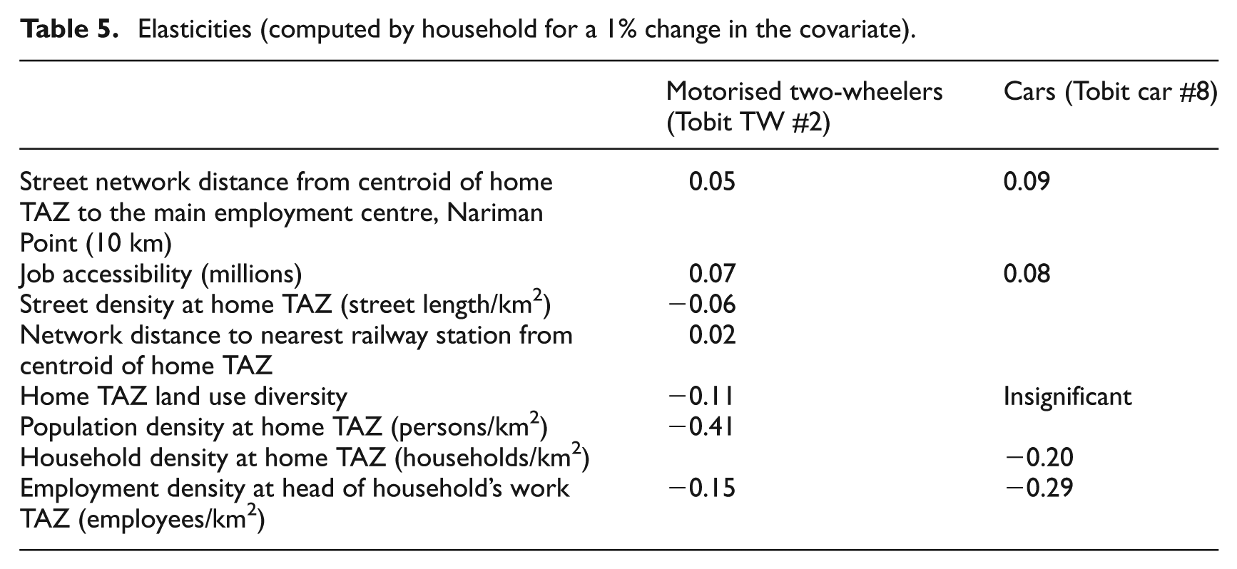
The average elasticity for land use diversity suggests that policies encouraging land use mixing may bring down private vehicle use, a finding validated by Ewing and Cervero (2010: table A-2). Housing and employment density elasticity values are comparable with Chatman (2003) whose dependent variable was commercial VKT (Ewing and Cervero, 2010: table A-1). Overall, the density elasticity findings for Mumbai are bigger than other studies, even though the covariates are computed using average density (section ‘Land use measures’). If more research on Asian cases corroborates these findings, policies may be considered to include density as a tool for managing private travel.

Policy discussion and implications for South and Southeast Asia

Most analyses of the built environment and vehicle use are in the Americas and Europe (Ewing and Cervero, 2010). These studies largely suggest that expanding metropolitan areas increase car use, and land use policies have marginal impacts for managing growing VKT. Fewer studies have looked at rapidly changing Asian cities (e.g. Yagi et al., 2013), where land development policies might affect residential and travel choices differently. Some Asian case studies shed light on car ownership and use, and support the idea that the well-off live in central cities and use private modes of travel (e.g. Li et al., 2010). Scholarship on Chinese cities has other interesting case-specific results, showing that city expansion is linked to higher car use (Pan et al., 2013). Findings about Indian travellers regarding cars corroborate other developing country scholarship on this topic, showing that improving socio-economic conditions predict car ownership and use (Rajagopalan and Srinivasan, 2008; Srinivasan et al., 2007). However, South and Southeast Asian countries also have the motorised two-wheeler, offering a cheaper form of private travel; a mode likely to grow given the rising incomes.

Motorised two-wheeler modes improve mobility but also have the potential to add to pollution and emissions (Iyer and Badami, 2007). As South and Southeast Asia urbanises with limited travel options in the peripheries, studying TW use impacts is becoming important (Dissanayake and Morikawa, 2010; Srinivasan et al., 2007; Yagi et al., 2013). This Mumbai study sheds light on the differing geography of car use versus motorcycle/scooter use. The finding that cars are used in urban centres, while scooters and motorcycles are used in the peripheries (Figure 1), suggests that subregional policies across large metropolitan areas are appropriate for managing vehicle growth. For example, after further research considering both the efficiency and equity aspects, differing taxes on ownership and use of vehicles by mode and subgeography could be developed.

From a land use perspective, the findings on density (Table 3, model #2 and Table 4, model #8) suggest that policies encouraging density have the potential to bring down vehicle use marginally. However, these findings require further validation from developing world cases, particularly in South and Southeast Asia. The outcome that incentivising land use mixes is linked to lower vehicle use is consistent with the broad literature, though the impact is predicted to be modest. This paper suggests that increasing transit supply has the potential for bringing down private vehicle use. However, only rail station proximity is tested here, and it is likely that further studies that include a full suite of travel options including jitneys may reveal bigger impacts from supplying formal (and supporting informal) transit.

Overall, the findings from the Mumbai case are promising for policies to reign in vehicle use in developing countries, though the impacts are marginal. The transportation findings suggest that greater destination accessibility by private modes increases vehicle use yet transit supply may bring down vehicle use. The land use findings indicate that density and land use diversity can reduce vehicle use, but as household distance from major employment zones increases, vehicle use may go up. These outcomes need to be corroborated from other Asian case studies that include better land use and transportation network data.

Footnotes

Appendix

Appendix 2.

Car, Pearson’s Correlations (N ≈ 842).

	ODISTNMPTNTREDLN	WKISMUMDM	HHTZAI082CARTTLEMPLFN	HHTZDI	HHPRKM2LN	UPETZTTLEMPLDENCRSLN	HHEUDISTSTAT250MTDM	PRCPTHHINCLN	EDUCDM	RESTYPDM	TOTALADULTSLN	CHILDYNDMHH	CARAVILPERTTLPRSNS	ENV	SBC
VKTCARHHBPLUS1LN	0.138**	0.04	0.108**	0.019	−0.062	−0.058	−0.057	0.03	0.029	0.056	0.075*	0.003	−0.009	0.017	−0.041
ODISTNMPTNTREDLN		−0.682**	0.051	0.143**	−0.247**	−0.284**	−0.109**	−0.119**	−0.05	0.029	0.045	0.074*	−0.216**	0.087*	0.358**
WKISMUMDM			−0.092**	−0.083*	0.244**	0.305**	0.091**	0.053	0.021	−0.059	0.007	−0.065	0.170**	−0.124**	−0.318**
HHTZAI082CARTTLEMPLFN				−0.009	0.207**	0.219**	−0.002	−0.043	−0.019	−0.070*	−0.012	0.004	−0.019	−0.234**	0.041
HHTZDI					−0.026	−0.01	−0.104**	−0.022	0.05	−0.074*	−0.021	0.001	0.001	−0.239**	−0.147**
HHPRKM2LN						0.369**	0.126**	0.044	0.065	−0.074*	0.025	−0.007	−0.011	−0.116**	−0.130**
UPETZTTLEMPLDENCRSLN							0.03	0.070*	0.014	−0.021	−0.019	−0.095**	0.078*	−0.229**	−0.147**
HHEUDISTSTAT250MTDM								−0.045	0.012	−0.074*	0.024	−0.008	−0.015	−0.098**	0.055
PRCPTHHINCLN									0.187**	0.155**	−0.099**	−0.265**	0.324**	0.526**	−0.229**
EDUCDM										0.105**	−0.176**	−0.075*	0.202**	0.340**	−0.127**
RESTYPDM											−0.021	0.041	0.049	0.416**	0.079*
TOTALADULTSLN												−0.155**	−0.543**	0.167**	0.051
CHILDYNDMHH													−0.438**	0.077*	0.080*
CARAVILPERTTLPRSNS														−0.073*	−0.184**
ENV															−0.017

Correlation is significant at the 0.01 level (2-tailed).

Correlation is significant at the 0.05 level (2-tailed).

Acknowledgements

This work benefited from commentary made by Allie Thomas, Elizabeth Deakin, Erick Guerra, Jake Wegmann, Miriam Aranoff, Rebecca Sanders, Robert Cervero and three anonymous reviewers. Akshay Vij and Amy Kim helped with critiquing the models. The Mumbai Metropolitan Regional Development Authority (MMRDA) shared the household travel survey data set.

Funding

The University of California Transportation Center’s Dissertation Grant and the Dean’s Normative Time Fellowship at the University of California, Berkeley, provided funding for this research.

References

Bento

Cropper

Mobarak

. (2005) The effects of urban spatial structure on travel demand in the United States. The Review of Economics and Statistics 87(3): 466–478.

Bertaud

Brueckner

(2005) Analyzing building-height restrictions: Predicted impacts and welfare costs. Regional Science and Urban Economics 35(2): 109–125.

Bhagat

Jones

(2013) Population change and migration in Mumbai metropolitan region: Implications for planning and governance. Asia Research Institute, National University of Singapore, Working Paper Series No. 201 (May).

Bhat

Guo

(2007) A comprehensive analysis of built environment characteristics on household residential choice and auto ownership levels. Transportation Research Part B 41(5): 506–526.

Brownstone

Fang

(2014) A vehicle ownership and utilization choice model with endogenous residential density. The Journal of Transport and Land Use 7(2): 135–151.

Brueckner

Sridhar

(2012) Measuring welfare gains from relaxation of land-use restrictions: The case of India’s building-height limits. Regional Science and Urban Economics 42(6): 1061–1067.

Cao

X (Jason)

Mokhtarian

Handy

(2009) Examining the impacts of residential self-selection on travel behaviour: A focus on empirical findings. Transport Reviews 29(3): 359–395.

Cervero

(2007) Transit-oriented development’s ridership bonus: A product of self-selection and public policies. Environment and Planning A 39(9): 2068–2085.

Cervero

Murakami

(2010) Effects of built environments on vehicle miles traveled: Evidence from 370 US urbanized areas. Environment and Planning A 42(2): 400–418.

10.

Chatman

(2003) How density and mixed uses at the workplace affect personal commercial travel and commute mode choice. Transportation Research Record: Journal of the Transportation Research Board 1831: 193–201.

11.

Chatman

(2009) Residential choice, the built environment, nonwork travel: Evidence using new data and methods. Environment and Planning A 41(5): 1072–1089.

12.

Dissanayake

Morikawa

(2010) Investigating household vehicle ownership, mode choice and trip sharing decisions using a combined revealed preference/stated preference nested logit model: Case study in Bangkok metropolitan region. Journal of Transport Geography 18(3): 402–410.

13.

Ewing

Cervero

(2010) Travel the built environment. Journal of the American Planning Association 76(3): 265–294.

14.

Ewing

Hamidi

(2014) Longitudinal analysis of transit’s land use multiplier in Portland (OR). Journal of the American Planning Association 80(2): 123–137.

15.

Ewing

Hamidi

Gallivan

. (2014) Structural equation models of VMT growth in US urbanised areas. Urban Studies 51(14): 3079–3096.

16.

Ewing

Tian

Goates

. (2015) Varying influences of the built environment on household travel in 15 diverse regions of the United States. Urban Studies 52(13): 2330–2348.

17.

Government of India (Ministry of Urban Development) (2012) Compendium of Projects and Reforms Under Jawaharlal Nehru National Urban Renewal Mission. July. Available at: http://jnnurm.nic.in/wp-content/uploads/2012/11/Compendium-Projects-amp-Reforms-JnNURM-MoUD-July-12-Vol-01Part-01.pdf (accessed 25 August 2015).

18.

Government of India (The High Powered Expert Committee (HPEC) for Estimating the Investment Requirements for Urban Infrastructure Services) (2011) Report on Indian Urban Infrastructure and Services. Government of India, March. Available at http://icrier.org/pdf/FinalReport-hpec.pdf (accessed 25 August 2015).

19.

Guerra

(2014) The built environment and car use in Mexico City: Is the relationship changing over time?Journal of Planning Education and Research 34(4): 394–408.

20.

Guerra

(2015) The geography of car ownership in Mexico City: A joint model of households’ residential location and car ownership decisions. Journal of Transport Geography 43: 171–180.

21.

Houston

Boarnet

Ferguson

. (2015) Can compact rail transit corridors transform the automobile city? Planning for more sustainable travel in Los Angeles. Urban Studies 52(5): 938–959.

22.

(2014) Changing job access of the poor: Effects of spatial and socioeconomic transformations in Chicago, 1990–2010. Urban Studies 51(4): 675–692.

23.

Iyer

Badami

(2007) Two-wheeled motor vehicle technology in India: Evolution, prospects and issues. Energy Policy 35(8): 4319–4331.

24.

Koenker

(2008) Censored quantile regression redux. Journal of Statistical Software 27(6): 1–25.

25.

LEA International Limited, LEA Associates South Asia Private Limited and Mumbai Metropolitan Region Development Authority (2008) Comprehensive Transportation Study for Mumbai Metropolitan Region. Final Report and Annexures. Canada and India. Unpublished.

26.

Walker

Srinivasan

. (2010) Modeling private car ownership in China: Investigation of urban form impact across megacities. Transportation Research Record: Journal of the Transportation Research Board 2193: 76–84.

27.

Long

(1997) Regression Models for Categorical and Limited Dependent Variables. Thousand Oaks, CA: SAGE Publications.

28.

Mumbai Metropolitan Region Development Authority (MMRDA) (2015) Projects, Transport. Available at: http://mmrda.maharashtra.gov.in (accessed 25 August 2015).

29.

Nallathiga

(2005) The impacts of density regulation on cities and markets: Evidence from Mumbai. International Journal of Regulation and Governance 5(1): 13–39.

30.

Pan

Shen

Zhao

(2013) Travel and car ownership of residents near new suburban metro stations in Shanghai, China. Transportation Research Record: Journal of the Transportation Research Board 2394: 63–69.

31.

Phadke

(2013) Mumbai metropolitan region: Impact of recent urban change on the peri-urban areas of Mumbai. Urban Studies (51)11: 2466–2483.

32.

Phadke

(2014) As toll roads face fire, Bandra-Worli sea link struggles for a profit. The Indian Express, 7 May. Available at: http://indianexpress.com/article/cities/mumbai/as-toll-roads-face-fire-bandra-worli-sea-link-struggles-for-a-profit/99/ (accessed 25 August 2015).

33.

Portnoy

(2003) Censored regression quantiles. Journal of the American Statistical Association 98(464): 1001–1012.

34.

Rajagopalan

Srinivasan

(2008) Integrating household-level mode choice and modal expenditure decisions in a developing country: Multiple discrete-continuous extreme value model. Transportation Research Record: Journal of the Transportation Research Board 2076: 41–51.

35.

Rajamani

Bhat

Handy

. (2003) Assessing impact of urban form measures on nonwork trip mode choice after controlling for demographic and level-of-service effects. Transportation Research Record: Journal of the Transportation Research Board 1831: 158–165.

36.

Salon

Boarnet

Handy

. (2012) How do local actions affect VMT? A critical review of the empirical evidence. Transportation Research Part D 17(7): 495–508.

37.

Schwanen

Lucas

(2011) Understanding auto motives. In: Lucas

Blumenberg

Weinberger

(eds) Auto Motives: Understanding Car Use Behaviors. Bingley, UK: Emerald Group Publishing Limited, pp. 3–28.

38.

Shirgaokar

(2014) Employment centers and travel behavior: Exploring the work commute of Mumbai’s rapidly motorizing middle class. Journal of Transport Geography 41: 249–258.

39.

Singh

(2010) Employment situation in Mumbai: An analysis. Global Labour Conference, Berlin, Germany, September. Available at: http://www.global-labour-university.org/fileadmin/GLU_conference_2010/papers/44._Employment_situation_in_Mumbai_An_analysis.pdf (accessed 25 August 2015).

40.

Society of Indian Automobile Manufacturers (2015) Statistics, Domestic Sales Trends. Available at: http://www.siamindia.com/statistics.aspx?mpgid=8&pgidtrail=14 (accessed 25 August 2015).

41.

Sridhar

(2010) Impact of land use regulations: Evidence from India’s cities. Urban Studies 47(7): 1541–1569.

42.

Srinivasan

Bhargav

Ramadurai

. (2007) Determinants of changes in mobility and travel patterns in developing countries: Case study of Chennai, India. Transportation Research Record: Journal of the Transportation Research Board 2038: 42–52.

43.

Yagi

Nobel

Kawaguchi

(2013) Time series comparison of joint mode and destination choice models in changing transportation environment, Jakarta, Indonesia. Transportation Research Record: Journal of the Transportation Research Board 2394: 100–110.

44.

Zegras

(2010) The built environment and motor vehicle ownership and use: Evidence from Santiago de Chile. Urban Studies 47(8): 1793–1817.

45.

Zhou

Kockelman

(2008) Self-selection in home choice: Use of treatment effects in evaluating relationship between built environment and travel behavior. Transportation Research Record: Journal of the Transportation Research Board 2077(1): 54–61.