
Abstract
This paper applies a general spatial equilibrium model to investigate the effect that distance within the urban hierarchy can have on interurban house prices. Our spatial model predicts a negative price gradient towards higher-tier cities, which can be decomposed into a ‘productivity component’ and an ‘amenity component’, representing respectively the effect of wage differences and households’ valuation of access to higher-order services. The theoretical findings are tested on data for the hierarchical urban system of the Pan-Yangtze River Delta in China. Both central and subcentral cities are shown to impose statistically significant distance penalties on interurban house prices, even after we control for amenities and characteristics that are generally considered to be the determinants of house prices. According to the empirical decomposition, the negative house price gradients are largely accounted for by the productivity component.
Introduction
House prices vary significantly across areas. For example, the average house price for the US metropolitan statistical areas (MSAs) in the top price decile in 2000 was about 290,000 dollars, almost four times the average for the MSAs in the bottom decile and more than twice the mean value. 1 Likewise, developing economies such as China exhibit a huge house price differential between cities. According to the ‘100 city house price index report’, 2 the 90th percentile price for 95 prefecture cities (municipalities) in December 2010 was more than three times higher than the 10th percentile price.
The remarkable variation in house price across cities is usually attributed to differences in socio-economic conditions and amenities. Household income and population (changes), which directly influence housing demand, are often cited as key factors (e.g. de Bruyne and van Hove, 2013; Potepan, 1996). On the basis of time-series data, the long-run equilibrium relationship between house price and income has been established by many authors (e.g. Ashworth and Park, 1997), though others have cast doubt on its validity (Gallin, 2006). Some demographic characteristics, such as the share of foreigners, are also partly responsible for the variation in house price across cities (e.g. Ozanne and Thibodeau, 1983).
Urban households are willing to pay a premium to live in a city with better amenities. For instance, cities with a warm winter or cool summer are always expensive (e.g. Rappaport, 2007). In addition, man-made amenities, notably school quality and crime rate, have a significant effect on house prices (e.g. Gyourko and Tracy, 1991). 3 Topographical constraints and legal regulations, which determine the housing supply, can also affect house prices (e.g. Malpezzi, 1996). Furthermore, as we argue here, the relative location of a city should be taken into account when explaining interurban house price patterns. This paper demonstrates a persistent spatial pattern whereby differences in house prices tend to increase as the location shifts from the core city to peripheral cities.
The effect of location on the price of inner-city land (or houses) has been widely investigated since the pioneering work of Alonso (1964), Mills (1967) and Muth (1969). Their work predicted a negative effect of distance on price when moving away from the Central Business District (CBD). Empirical evidence for negative gradients of population density, house prices or land values has been found in studies of Chicago, Berlin, Stockholm, Beijing and the southern part of West Norway (Ahlfeldt, 2011; McMillen, 1996; Osland et al., 2007; Söderberg and Janssen, 2001; Zheng and Kahn, 2008). The pattern of house prices in a modern polycentric city is much more complicated, however. There, location is also shaped by proximity to subcentres and other important nodes such as universities, hospitals and parks (Heikkila et al., 1989; Qin and Han, 2013; Waddell et al., 1993).
In an interurban context where cities form a hierarchy, 4 it is no surprise to find that house prices in top-tier cities tend to be the highest, whereas lower prices characterise the lowest-order cities in the hinterland. Yet relevant studies on the effect of a city’s location on house prices are largely absent; to our knowledge, only two have been published. De Bruyne and van Hove (2013) developed a theoretical model to explain, from the perspective of commuters, how access to a core municipality will affect house prices. The underlying premise is that commuters have to compensate for their loss in leisure time and for the cost of the journey to work by economising on housing expenditure. Using municipal-level data for Belgium, they found solid evidence supporting their hypothesis: good access to economic centres (capital city or provincial capitals) will increase house prices.
Commuting between core and peripheral cities might not be realistic in some countries. In this regard, Partridge et al. (2009) present a general analytical framework that combines the spatial general equilibrium framework of Roback (1982) and Central Place Theory. They state that location characteristics (access to higher-tier centres) will enhance a firm’s profitability and households’ utility, respectively, by providing access to greater markets and unique consumer services such as exotic restaurants, renowned museums and specialised healthcare facilities. Spatial differences in house prices are thus outcomes of the location responses of firms and households to the urban hierarchy. Data for rural and urban counties in the USA shows that estimated incremental distance penalties for remoteness from the combined tiers of the urban hierarchy are about 12% to 17%. 5
In the study underlying this paper, we systematically investigated how the location of a city – i.e. distance to higher tiers within the urban hierarchy – would affect house prices by applying a general spatial equilibrium framework analogous to that of Partridge et al. (2009). This framework predicts a negative interurban house price gradient with respect to higher-tier cities. The price gradient can be decomposed into a ‘productivity component’, which represents the effects of wage difference caused by agglomeration spillovers, and an ‘amenity component’, which reflects households’ valuation for access to higher-tier consumer services. We used aggregate data from China’s Pan-Yangtze River Delta, where a housing market has emerged and matured since the housing system reform was launched in 1998. With that data, a series of interurban house price gradients were estimated and empirically decomposed after controlling for city-specific amenities and characteristics.
The contribution we intend to make with this paper is twofold. First, we test the penalties imposed by distance within the urban hierarchy on house prices in developing countries where the spatial pattern of interurban house prices has been largely understudied. Second, we attempt to decompose the house price gradient rather than wage (growth) differentials, the latter having been analysed previously by Partridge et al. (2010).
Related literature
Explaining house price differences across markets has long been a concern, as amply demonstrated in the literature. 6 Ozanne and Thibodeau (1983) developed an implicit demand and supply model of metropolitan housing markets. The markets were divided into rental and homeowner sectors, which are linked by tenure choice and the urban land market. Reduced equations for house prices and rents were then estimated using seemingly unrelated regression (SUR) method based on a data set of MSAs in the USA. Among other independent variables, they considered median income, number of households, demographic characteristics, tax, construction cost, price of land and other consumer goods, as well as geographic features and government restrictions on land supply. Surprisingly, they found that two variables, namely income and number of households, significantly affect rents but not house prices. Coastal location, as a proxy for topographical land use restrictions, had no influence on house prices either. Potepan (1996) further extended the framework of Ozanne and Thibodeau (1983) to include housing service, housing capital and urban land markets, of which the first two are linked through user-cost relationships. In contrast, their reduced-form estimates based on data for MSAs confirm the significant effect of income and population (change) on house prices. Amenities, such as climate and quality of public services, were also shown to influence house prices. Using a provincial panel data set for China, Li and Chand (2013) also found that income level and the ratio of impending marriage population to total population have a significant effect on house prices.
While most of the studies include income and population as independent variables, the spatial general equilibrium framework (Glaeser et al., 2006; Roback, 1982) clearly justifies the endogeneity between wage, population and house prices. This framework accommodates migration across markets to equalise the interurban utility level. Accordingly, price differences between cities are considered as compensating differentials that compensate for city amenities. The implicit prices of amenities can further be used to calculate a quality-of-life index. Gyourko and Tracy (1991) regressed housing expenditure on a set of pure amenities such as climate and environmental indicators and a set of non-pure amenities such as education, safety and healthcare. In general, they found that those amenities, as a group, significantly affect housing expenditure in the USA. Similarly, Rappaport (2007) provides evidence from the US market that counties with warmer winters and cooler summers enjoy higher growth in house prices. Not surprisingly, amenities are also highly valued in Chinese housing markets. For example, green space and beach access have a positive relationship with house prices, while air pollution, measured as particulate matter (PM), affects house prices negatively (Zheng et al., 2010). Moreover, cross-boundary pollution flows, referring to pollutants carried by wind from other cities, also have a negative effect on a specific city’s house prices (Zheng et al., 2014).
On the supply side the price of raw land and construction cost are the two main factors, playing an even bigger role in explaining house prices in more developed cities (Li and Chand, 2013). Conditions such as topographical features and regulation constraints, which may be directly or indirectly correlated with land prices and construction cost, can also affect house prices. When facing a demand shock, cities with a relatively elastic supply will experience a modest house price increase because of the unfettered new supply. On the other hand, house prices must rise dramatically in cities with an inelastic supply (Glaeser et al., 2006). Malpezzi (1996) investigated the relationship between the regulatory environment, as measured by a series of rent controls and zoning plans, and housing markets in the USA and found that regulation raises rents and house prices but lowers homeownership rates. The finding that greater regulatory restrictiveness will increase house prices or foster a larger house price growth in a booming period is further confirmed by Ihlanfeldt (2007) and Huang and Tang (2012), among others.
More recently, some studies have considered the spatial dimension of house price determinants. A few authors have investigated the role that the relative location of a city within the urban hierarchy plays in forming house prices, assuming that central cities that have larger market potential and higher consumer amenities will have a positive effect on nearby cities’ house prices (de Bruyne and van Hove, 2013; Partridge et al., 2009). Our study will contribute to this stream of research by investigating the effect of distance within the urban hierarchy on interurban house prices in an emerging market – China.
Theoretical framework
Our theoretical framework follows the spatial general equilibrium model of Roback (1982), which has been extensively used by Beeson and Eberts (1989) and Partridge et al. (2010). To perform our analysis, we made several assumptions. Both capital and labour can move freely across cities, thereby allowing individuals to select their residential location within a particular city and to choose between different cities. However, the option of living in one city and working in another is ruled out. Further, land is fixed in each city but can be freely changed between uses.
Households maximise utility subject to a budget constraint by choosing amounts of traded composite goods (

where

The indirect utility function has the usual properties,
Suppose that land is the only input of housing production according to a constant-return-to-scale production function:

where
Following the tradition of Rosen (1979), households are viewed as self-producers of composite goods. The assumption of self-production ensures that land is not a factor of production. That is,

The unit cost function
Now we turn to the effect that distances in the urban hierarchy (
Holding within-area amenities (
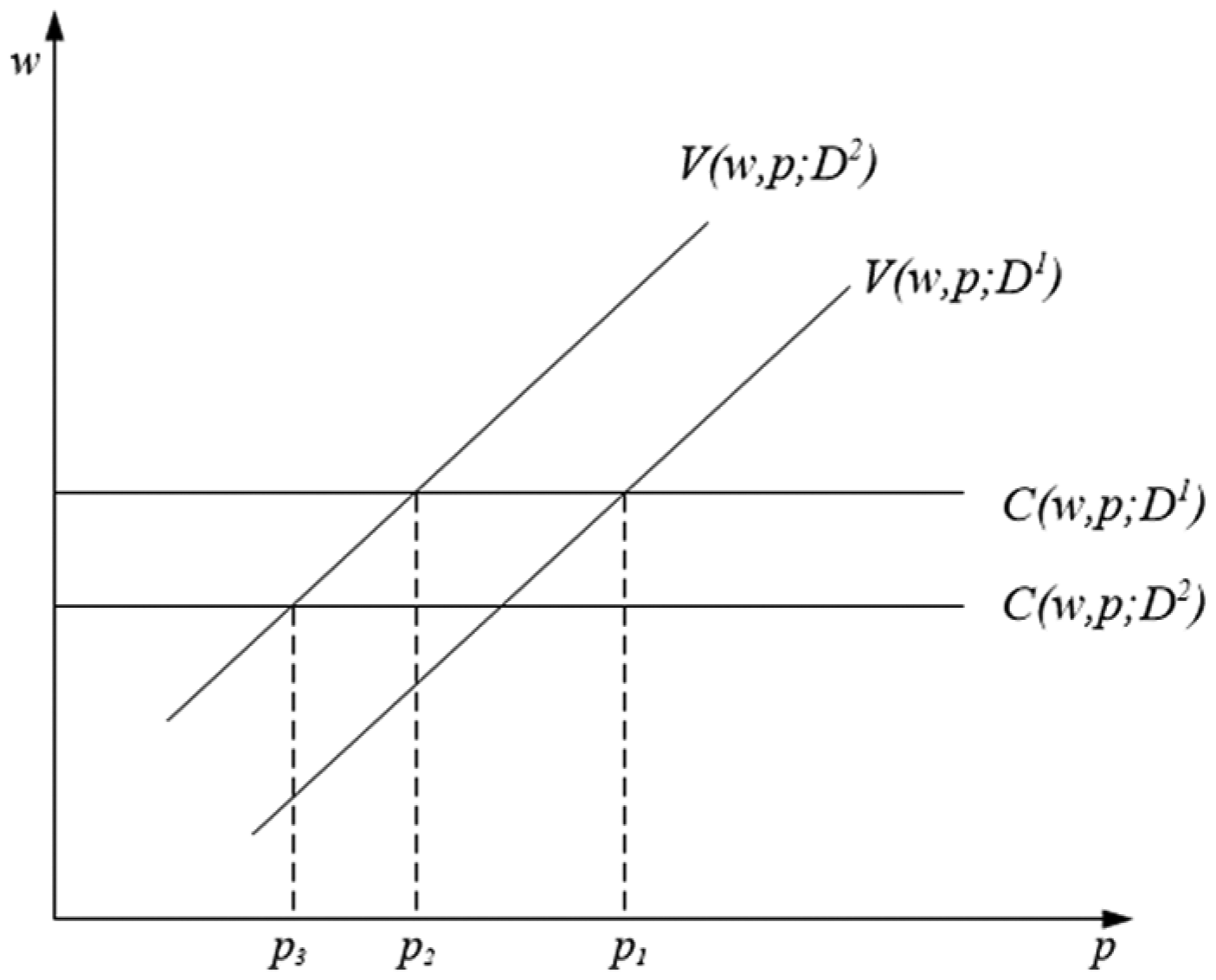
Illustration of distance effects on equilibrium wages and house prices.
Totally differentiating the equations (2), (3) and (4) and solving for
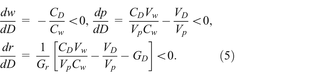
Rearranging
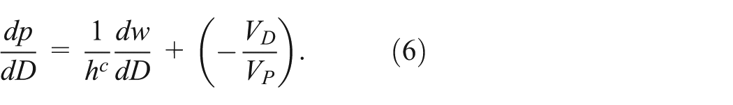
The first term in Equation (6) is the effect on
where
Hierarchical urban system and empirical data
Hierarchical urban system of interest
Prior to introducing the readers to the hierarchical urban system covered in this study, we offer some background on the administrative arrangement of Chinese urban areas. A typical prefecture city, or a municipality directly under the central government (municipality for short), usually consists of districts and counties (or county-level cities). The ‘city proper’ (shiqu) of the prefecture city is made up of the districts (Ding, 2013). 7 The hierarchical urban system mentioned in this paper pertains to the city proper of prefecture cities and municipalities.
The empirical grounds for the study refer to the hierarchical urban system of the Pan-Yangtze River Delta (PYRD). The area comprises one municipality (Shanghai) and three provinces (Jiangsu, Zhejiang and Anhui), including 42 cities, with a land area of 350,000 km2 and a population of 215 million in 2010 (see Figure 2). With the hukou restriction on labour mobility being phased out in the transition to a market economy, a more liberal labour market has emerged. People can freely migrate to cities that offer higher real wages or better urban amenities. For example, the population of Shanghai increased by 43% from 2000 to 2010. Furthermore, urbanites tend to live and work in the same city because of cultural traditions, the expense of commuting and so on. Given these features, the PYRD constitutes a natural experimental setting for our theoretical analysis.
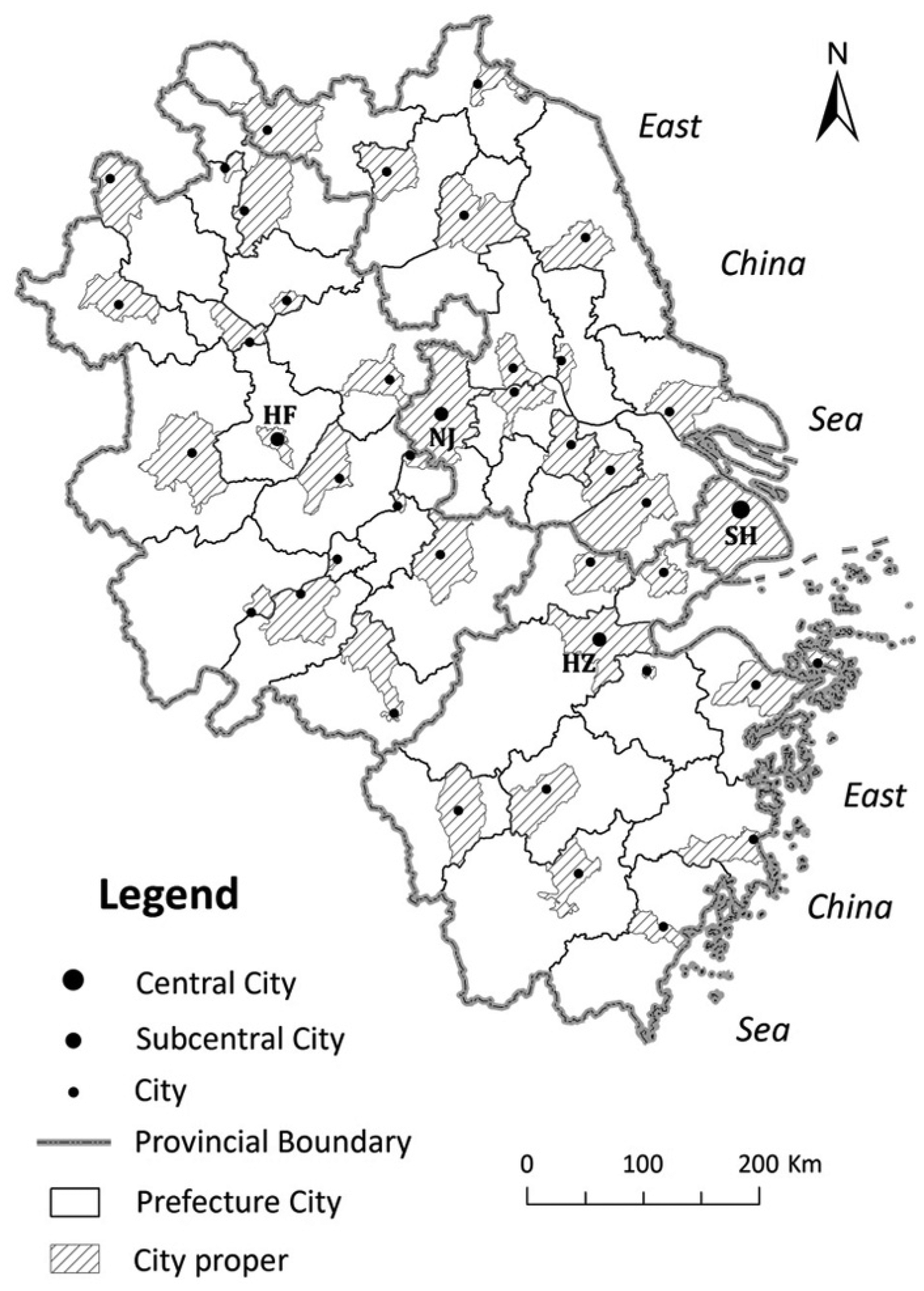
Hierarchical urban system of Pan-Yangtze River Delta.
Accompanying the rapid economic growth and liberalisation of the labour market, the increasing urban population has been accommodated in a modern, market-oriented housing sector since the housing reform of 1998. Three types of housing are provided to meet the demand of different income groups: commercial housing, government-supported affordable housing (Jingji shiyong fang) and government-subsidised rental housing (Lianzu fang) (Wang et al., 2012). The commercial sector is market-oriented. At present, it comprises the majority of the units, even though affordable housing has been encouraged and supported by governments in recent years.
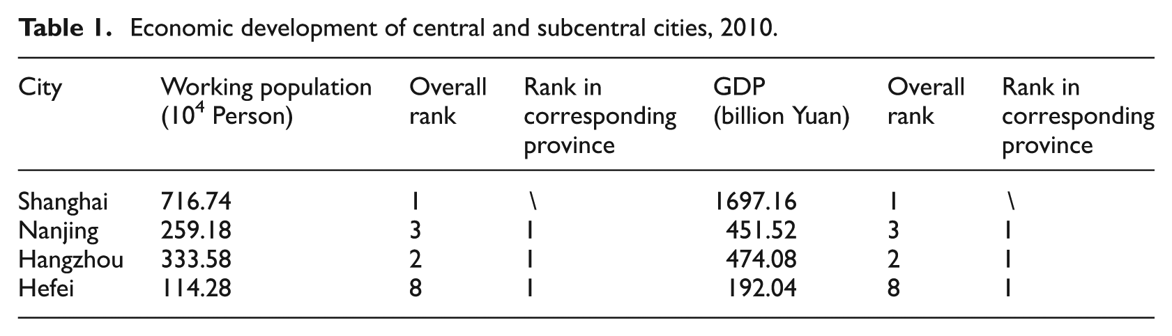
In theory, a higher-tier city should have a relatively large market and provide higher-order services and products for lower-tier cities. In China, urban development and the spatial layout of cities are usually guided by the upper-level governments’ plans. Therefore, the Outline of National Urban System Planning (2005–2020) offers a good perspective from which to define the urban hierarchy in the PYRD area. The Outline identifies a three-tiered urban system. Shanghai, planned to be the nationwide central city, is undoubtedly the only highest-tier city. Nanjing, Hangzhou and Hefei, as local-central cities and the capitals of Jiangsu, Zhejiang and Anhui province, respectively, comprise the second (subcentral) tier. They offer higher-order functions and services for third-tier cities. Note that Ningbo, designated as a local-central city, is excluded from the list of subcentral cities. Because Ningbo lies very close to Hangzhou, its influence on third-tier cities can be easily overshadowed by Hangzhou. 8 The evidence presented in Table 1 suggests that the inclusion of Hefei as a subcentral city is a little controversial; its economic indicators, namely the working population and GDP, are not in the top rank. However, considering its leading position in Anhui province, it is reasonable to define Hefei as one of the local centres.
Economic development of central and subcentral cities, 2010.
Model specification and data
We use a set of panel data for 42 cities (41 prefecture cities and one municipality) spanning the period from 2006 to 2010. Thus, we have 210 annual observations. According to the theoretical model, the full specification of the pooled cross-sectional model can be expressed as:
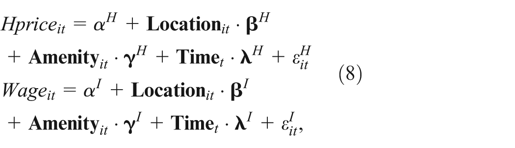
where
The primary data sources for this paper are the city-level or province-level statistical yearbooks as well as China City Statistical Yearbooks. Here, the notion of house price refers to the average sale price of newly sold residential buildings per square metre of floor space in the city proper. 9 This measure includes both finished and pre-sale housing. 10 One drawback of this measure is that it does not control for housing quality. Nonetheless, to our knowledge, this is the only aggregate measure of house price that can cover all of the cities in this analysis. The wage level is approximated by annual average wages of employees working in state-owned, collective-owned non-private sectors. The wage data is gathered from China City Statistical Yearbooks.
Both geographical distance and travel time are used to measure the accessibility of a city to higher-tier cities. Geographical distance is the straight line distance between the CBD of two cities, while travel time means the least amount of driving time extracted from Google Maps in December 2012. By the same approach, geographical distance and travel time to the nearest subcentral city are constructed. Our measure here differs from the incremental distance (see note 5 for a detailed explanation) of Partridge et al. (2009). Under the assumption of incremental distance, a third-tier city, say city
A set of variables are chosen as proxies for city amenities and characteristics. The main climate variable is the winter temperature, specifically the average temperature of December, January and February. The summer temperature is excluded, as it does not vary much across our study area. The environmental indicator is the annual amount of industrial smoke and dust emissions per GDP. Smoke and dust are the two major components of particulate matter, which is an important aspect of quality of life. This measure reflects the intensity of particulate matter emissions. Higher emission intensities usually indicate a higher share of the polluting sector in the industrial composition, which will make the city less pleasant to live in. We also create the dummy variable ‘coastal city’ to measure the living comfort of a city. It takes the value of 1 if the city proper borders an ocean but the value of 0 otherwise. The man-made amenities we consider are healthcare and education conditions, the most important aspects of quality of life in a city. They are approximated by the ratio of students to teachers and the number of physicians per thousand inhabitants. Finally, the variable ‘arable land per capita in 2004’ is incorporated as a proxy for planning and regulation constraints. To ensure grain security, the central government has drawn a ‘red line’ minimum for arable land at 120 million ha in the whole country. In this regard, a city with less arable land will probably face more strict planning and regulation constraints, which will consequently push up the house prices but limit its population growth (Glaeser et al., 2006). Note that the spatial context of winter temperature, smoke and dust emissions, and arable land per capita does not pertain to the city proper but covers the whole prefecture city (including counties or county-level cities). 11
Estimating interurban house price gradients
A set of interurban house price gradients were estimated to investigate the distance penalties of central and subcentral cities. First, a parsimonious model that only considers the effect of a central city was estimated based on three distance-decay forms. Second, the augmented models that contain both central and subcentral cities were used to detect the house price pattern in a polycentric urban system. Third, after controlling for city amenities and characteristics, the house price gradients of central and subcentral cities were re-estimated.
House price gradient towards central city
Specifying the functional form is an important issue in empirical analysis. In order to choose the ‘best’ model specification, we considered three distance-decay forms of parsimonious models: linear (Level-Level), semi-log (Log-Level) and log-log (Log-Log). In addition, we included two regional dummy variables to control for the provincial fixed effects of Jiangsu and Anhui, such as natural resource availability and policy difference.
The estimated central-city house price gradients are reported in Table 2. t statistics were produced on the basis of standard errors clustered by city that are robust to correlation between error terms of the same city and heteroskedasticity over time. Except for the linear functional form where the negative coefficients of distance measures are not significant, both the semi-log and log-log form detected the highly significant distance penalties of the central city (Shanghai) on house prices in other cities. These penalties are in accordance with our theoretical findings as well as findings in US housing markets. To our surprise, geographic distance performs even better than travel time, which is considered to be more appropriate for measuring the accessibility between cities. The explanation may be related to the fact that the travel time has changed along with the continuous improvement of transportation infrastructure in the study area. However, what we actually used is a constant travel time derived from Google Map service, which could not track such changes. 12 The following analysis only takes geographical distance into account.
Estimation of house price gradient towards central city.
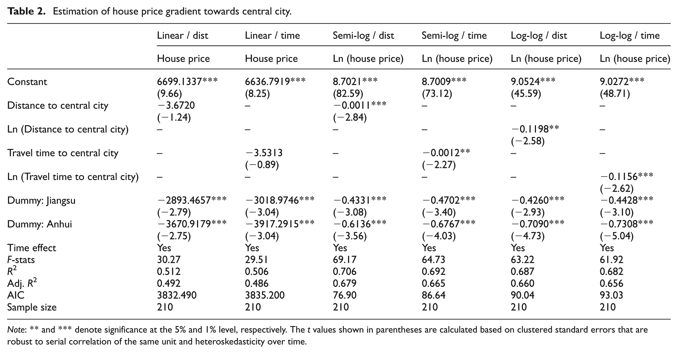
Note: ** and *** denote significance at the 5% and 1% level, respectively. The
The semi-log functional form using geographical distance performs best, according to the goodness-of-fit and AIC criteria. Together with two regional dummy variables, the geographic distance to the central city can explain 70% of the spatial variance of house prices in this model. The corresponding negative gradient is −0.0011, indicating that for 1 km further away a city lies from the central city, the average house price will decrease by about 0.11% when holding the regional effects constant. Moreover, house prices in Jiangsu province are significantly lower than those in Zhejiang, and Anhui is even cheaper. Finally, the estimation results of four time dummy variables show that overall house prices rose continuously during the study period, though we do not report the results. 13
House price gradient of both central and subcentral cities
To investigate the distance penalties of both central and subcentral cities on interurban house prices, we extended the framework of Heikkila et al. (1989), who considered the role of subcentres in a polycentric city. For our interurban augmented model, we assumed a competitive relationship among three subcentral cities but a complementary relationship between each of them and the central city. Thus, access to subcentral cities is measured by the distance to the nearest subcentral city. We then assigned either the semi-log or log-log distance-decay form to both central and subcentral cities, resulting in four models with different functional combinations.
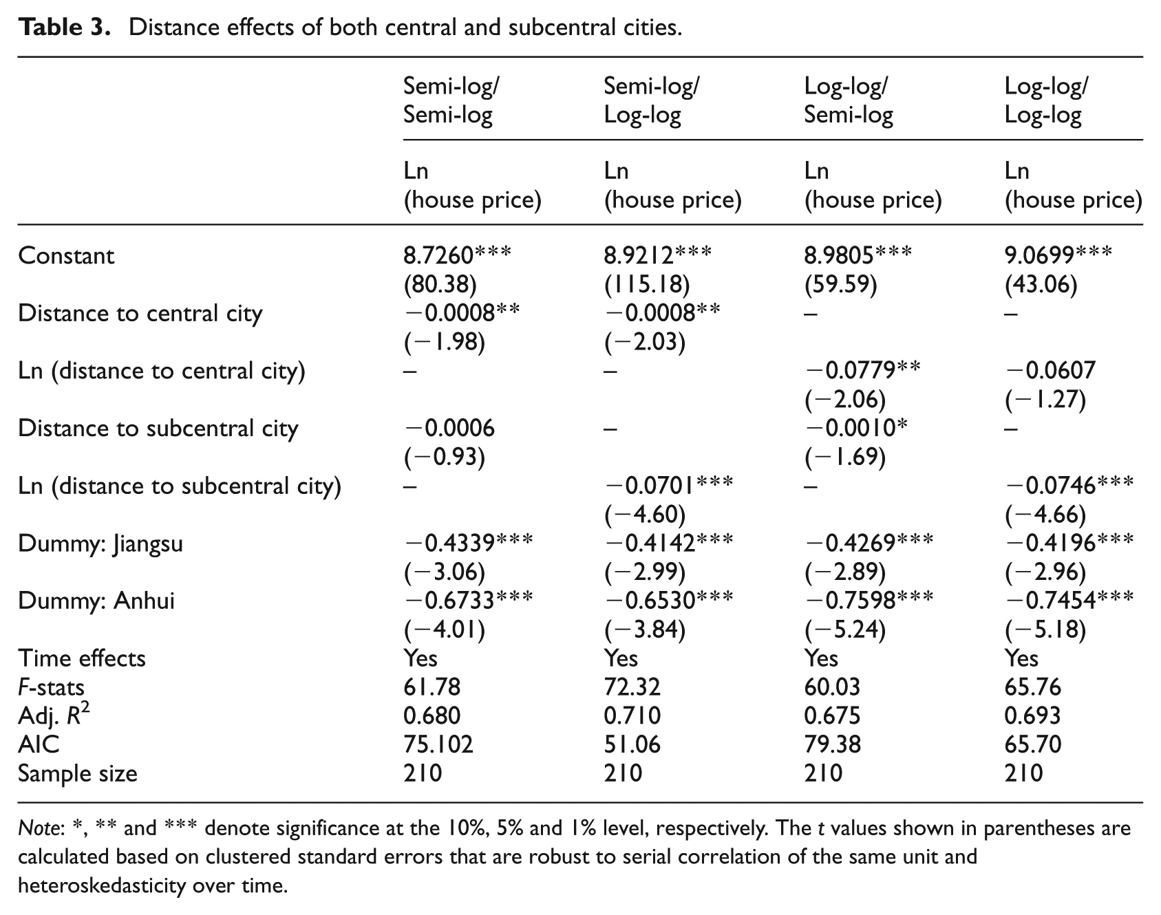
The results shown in Table 3 reveal that both central and subcentral cities have significantly negative distance effects on house prices when using the semi-log/log-log form and log-log/semi-log functional form. Those results also show that the semi-log/log-log form is the best one in terms of adjusted R2 and AIC criteria. However, the distance penalties are no longer significant, even at 10% significance level, for the central city in the log-log/log-log model or for the subcentral city in the semi-log/semi-log model. Thus, it is certainly correct to infer that the log-log function is more appropriate than the semi-log function for subcentral cities. It should be kept in mind that the central city always has a macro-effect that influences a larger radius while the subcentral city only has a local micro-effect. In that light, it seems that the choice of functional form is sensitive to the influence sphere of the centre. The log-log function performs better when the area of influence is relatively small, while the semi-log function is more appropriate if the area is larger. These findings are in line with those of Osland et al. (2007), who found that the exponential (semi-log) function performs best when the estimation is based on a large area, while the power (log-log) function performs best if the data is restricted to a small area.
Distance effects of both central and subcentral cities.
Note: *, ** and *** denote significance at the 10%, 5% and 1% level, respectively. The
Unlike the semi-log model that only includes the effect of the central city, adding the effects of subcentral cities raises the adjusted R2 from 0.679 to 0.710. Their added effects explain 3% more variance in interurban house prices and decrease the magnitude of the distance penalties of the central city by about 27%. Since we use different functional forms for central and subcentral cities, we cannot compare the magnitudes of their distance penalties directly.
House price gradient after controlling for city amenities and characteristics
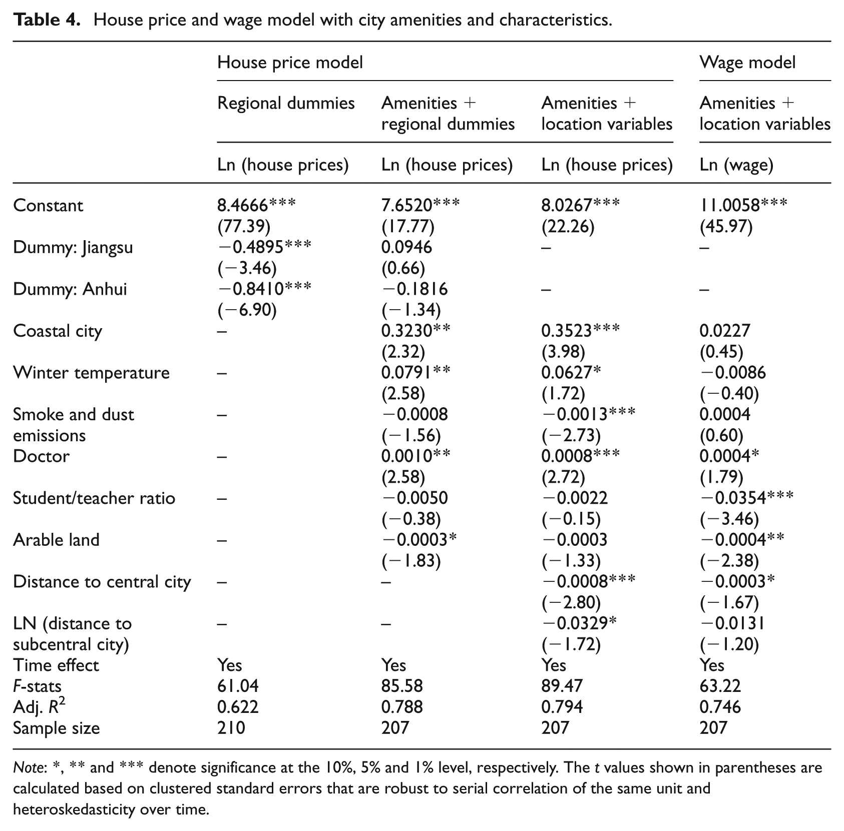
As suggested by the theoretical model, the negative house price gradient with respect to higher-tier cities should persist after controlling for city amenities and characteristics. Before estimating this, we first investigate the compensating house price differentials for urban amenities and characteristics. As noted earlier, the average house prices in Zhejiang, Jiangsu and Anhui provinces differ significantly from each other. This observation is further supported by the estimation results of column 1 in Table 4, which only contains two regional dummy variables. We assume that the observed house price differentials across provinces are actually proxies for the differences in amenities. The result of testing this hypothesis is shown in column 2 of Table 4. After including the variables of city amenities and characteristics, the regional effects of Jiangsu and Anhui province fall dramatically and are no longer significant, which offers some support for our hypothesis.
House price and wage model with city amenities and characteristics.
Note: *, ** and *** denote significance at the 10%, 5% and 1% level, respectively. The
The six variables of city amenities and characteristics, together with the two regional dummy variables, account for nearly 80% of the house price variance. As a group, the amenity and characteristic variables are statistically highly significant at the 1% significance level (the joint F-statistic is 39.98 where the 1% critical value is 2.90), and each has the anticipated sign. Among these variables, winter temperature, bordering an ocean and number of doctors have significantly positive effects, while arable land per capita has a negative effect at a significance level of 10% or better. The unpleasant effect of smoke and dust emissions is marginally insignificant.
The third column of Table 4 reports the estimation results of the model with both amenity variables and two distance measures. The two distance variables in which we are most interested still have significantly negative effects: distance to the central city is significant at the 1% level, while distance to the subcentral city at the 10% level. Compared with the semi-log/log-log model that only includes two distance variables and two regional dummies, the magnitude of the central-city house price gradient in this model does not change, but the distance penalties of the subcentral city decrease by about 50%. The point estimates of city amenities and characters are quite robust as they do not differ much from the results in column 2. Perhaps the most obvious change is that the negative effect of particulate matter becomes highly significant.
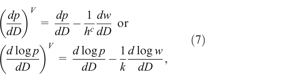
Decomposition of interurban house price gradient
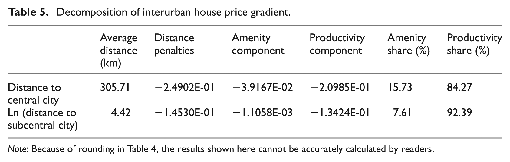
The previous section has provided estimates of the impact of urban hierarchy distances on house prices. According to the theoretical model, the decline in the interurban house price gradient could be attributed either to productivity disadvantages or amenity disadvantages. This section will empirically decompose the interurban house price gradient based on equation (7) and reveal which component contributes more to the negative price effects of remoteness from higher-tier cities.
In doing so, we first estimated the wage gradient, which is reported in the fourth column of Table 4. Overall, the distance and amenity variables perform less successfully in the wage model than in the house price model, given the lower adjusted R2 of wage regression. The central city still imposes a statistically significant distance penalty on wages, but its magnitude is less than the penalty on house prices. The negative coefficient of distance to subcentral cities, on the other hand, is no longer significant in the wage model. Among the significant wage determinants are two man-made amenities, namely the number of doctors and the ratio of students to teachers, as well as the area of arable land. Unlike the households, firms seem not to value the climate and environmental amenities as they are not significant in explaining wage differences. In contrast, firms strongly prefer man-made amenities, especially the human capital that is partially reflected in the student/teacher ratio. Of course, access to higher-tier cities is valued by both firms and households.
To decompose the house price gradient, we need to know the share of the household budget that is spent on housing (
With the parameter
Decomposition of interurban house price gradient.
Note: Because of rounding in Table 4, the results shown here cannot be accurately calculated by readers.
According to equation (7), our decomposition of the interurban house price gradient is sensitive to the parameter
Conclusion and discussion
While most studies have attributed the house price differences across cities to the differentials in city-specific amenities and characteristics, this paper focuses on the spatial dimension of the determinants of interurban house prices, i.e. the effect of urban hierarchy distance. We carried out our analysis under a general spatial equilibrium framework. Location decisions of firms and households jointly predict a declining pattern of house prices with distance from higher-tier cities. This negative house price gradient combines two aspects. First, firms in the higher-tier cities and their nearby areas are able to pay higher wages because of the productivity advantage, thereby driving up house prices. Second, households are willing to pay a premium on house prices for access to higher-order services. The theoretical findings are tested with the aggregate data of a specific hierarchical urban system in the Pan-Yangtze River Delta.
Both central and subcentral cities are found to impose statistically significant distance penalties on interurban house prices if we can correctly specify the distance-decay functions. The choice of forms for the functions is sensitive to the influential radius of the targeted higher-tier cities: the semi-log function is the best choice for the central city, while a log-log decay function is better for subcentral cities. The negative effects of urban hierarchy distance on house prices are robust, even after we control for city amenities and characteristics. We also find evidence of compensating house price differentials in terms of climate, environmental and healthcare amenities. The most counterintuitive finding embedded in the estimation of the central-city gradient – that the use of travel time does not improve the model’s performance – is probably due to the fact that our time-point measure cannot truly reflect the cost of travel and changes therein during the study period.
To decompose the house price gradient, the wage gradient is also estimated. The results show that distances to the central and subcentral cities have negative impacts on wages, though the penalties of subcentral cities are not statistically significant. In particular, the slopes of house price gradients are much steeper than those of wage gradients, which may be taken as preliminary evidence of the existence of an amenity premium. Yet, the decomposition results reveal that the ‘amenity component’ contributes very little; the ‘productivity component’ contributes strongly to the negative house price gradients. This discrepancy is in line with the wage (growth) gradient decomposition studies by Beeson and Eberts (1989) and Partridge et al. (2010), who also found that the productivity component was much more important in determining the wage (growth) differences. Although the decomposition results obtained in this study are conditional on devoting a relatively large share of the household expenditure to housing (
Our empirical findings should be interpreted with caution because of a few methodological flaws. First, owing to the general lack of data on housing markets, we chose to include only cities at the prefecture level (or above) of the PYRD hierarchical urban system. That choice limited the sample size and could thereby affect the robustness of the estimation results. Since some other city clusters have recently been growing rapidly in China, such as the Pearl River Delta and the Bohai Bay Economic Rim, future studies could be based on a large data set that combines all of these urban hierarchies. Second, studies on house price dynamics have suggested the existence of spatial interaction between intercity housing markets, which may result in spatial autocorrelation. Our failure to take this into account here may have led to inefficient estimators. In fact, the spatial autocorrelation of house prices has been extensively discussed in intracity studies (McMillen, 2010; Osland, 2010; Yu et al., 2007). Still, investigations of cross-sectional interurban housing markets are rather rare and warrant attention in the future. Third, we exclude land from the production of composite goods. That is, the benefits that accrue to households from having access to higher-tier cities will be completely capitalised in house prices and, in turn, in land prices. In the future, it would be interesting to investigate whether these benefits can also be capitalised in wages and whether urban hierarchy distance has a significant effect on land prices. China would provide a natural setting for testing the latter hypothesis because it has an explicit urban land market.
Footnotes
Acknowledgements
We appreciate the comments of three anonymous referees. We would like to thank participants of the Housing Economics workshop at the 2013 ENHR International Conference, in Tarragona, Spain for their commentary. And we are grateful to Marietta Haffner and Harry Boumeester for their help in calculating the share of expenditure on housing
Funding
Yunlong Gong would like to thank the China Scholarship Council (CSC) for providing the scholarship to support his study at Delft University of Technology.