Technological spillovers in space and firm productivity: Evidence from China’s electric apparatus industry

Abstract

Chinese

Using a spatial econometric model this article studies the determinants and spatial spillovers of firm productivity in China’s electric apparatus industry over the period of 1999–2007. We apply Kelejian’s FE-2SLS procedure to a higher-order spatial autoregressive model and estimate the spatial dependence of firm-level TFP within and across regional borders. The model demonstrates positive and significant intra-regional technological spillovers among firms. It also provides direct evidence that technological spillovers attenuate rapidly in spatial distance. We find that firm productivity benefits from own R&D and export activities, employment density, market competition and public expenditure. Further analyses show that the strength of spillover effects is affected by a broad range of factors, including the surface area of the region, administration type, border effect, transport and ICT infrastructure, FDI intensity, the financial sector, the utility service sector, and human capital. Factors that facilitate long-distance economic connections in general make inter-regional spillovers stronger but intra-regional spillovers weaker.

Keywords

agglomeration economic development public expenditure spatial autoregressive model spillover TFP

Introduction

Productivity isn’t everything, but in the long run it is almost everything. (Paul Krugman)

The sources of total factor productivity (TFP) growth have been widely debated in the literature from both macro and micro perspectives (see Syverson, 2011, for a survey and the references therein). Productivity differences at the micro level are usually attributed to various factors such as access to foreign markets (Clerides et al., 1998), firm-level innovation (Griffith et al., 2004), ownership structure (Aitken and Harrison, 1999) and external market conditions, especially agglomeration economies (Ciccone and Hall, 1996; Henderson, 2003). Great thinkers such as Marshall (1890) and Porter (1990) conceive agglomeration as the hotbed for industrial growth and firm performance. Since then, the NEG theory (Behrens et al., 2014; Duranton and Puga, 2004; Krugman, 1991) have developed multiple micro-foundations of agglomeration economies.¹

Despite the empirical success in identifying individual mechanisms, early literature implicitly treats agglomeration as a club good but overlooks the spatial interactions among firms. A major departure from this tradition was Rosenthal and Strange (2003), who investigated the geographic content of agglomerative spillovers using micro data. Since then spillover effects within and across the geographic boundary come into the limelight. At the micro level, spatial interactions are usually identified by estimating the benefits of agglomeration at varying distances (Arzaghi and Henderson, 2008; Rosenthal and Strange, 2003, 2008). Some researchers regress firm-level productivity on the characteristics (R&D, FDI, etc.) of neighbouring firms (Keller and Yeaple, 2009; Wei and Liu, 2006). These treatments, however, fail to provide direct evidence on the spatial dependence of firm-level productivity (or innovations in productivity).

This article contributes to the empirical literature on productivity analysis in several aspects. First, we conduct a rigorous analysis on the spatial dependence of firm-level productivity, and provide direct evidence of agglomerative spillovers. This is done with county-level geographic information and the China Industry Survey data set. Second, we implement a bootstrap version of Kelejian and Prucha’s (1998) FE-2SLS procedure that accounts for heteroscedasticity and spatial autocorrelation in the error term. We present empirical evidence that our method is superior to the RE-FG2SLS estimator adopted by some recent studies (e.g. Baltagi et al., 2015). Third, our empirical specification allows us to study separately the spillovers from different types of neighbours: those in the same region (intra-regional) and those in nearby regions (inter-regional). Later, we find that intra- and inter-regional spillover effects both respond to geographic and socio-economic factors.

Our spatial analysis controls for sources of productivity growth identified by the literature, especially Chinese studies. These include R&D activity, export behaviour, agglomeration, and public spending.

There is a long literature linking productivity with R&D activity (Hall et al., 2010) and export behaviour (Syverson, 2011). Empirical studies on China usually find a positive effect of R&D activity on productivity (Boeing et al., 2016; Hu and Jefferson, 2004; Hu et al., 2005), but those on export behaviour are by far inconclusive (Bao et al., 2015; Lu, 2010; Lu et al., 2010). Our study shows that a 10% increase in R&D activity and exports makes a firm 1.7% and 0.9% more productive, respectively.

Empirical researchers have proposed various measures for agglomerative effects.² In this study, we control for localisation economies, employment density, and competition. Firm-level evidence from developed economics suggests that productivity benefits from these factors (Henderson, 2003; Martin et al., 2011). Studies on Chinese data (e.g. Hu et al., 2015; Sheng and Song, 2013) seem to agree on the role of localisation, but have contrasting findings in competition. We find that firm productivity benefits strongly from employment density and competition, but not from localisation economies.

Following Aschauer (1989), we control for local public expenditure as another local market condition. We find that a 10% increase in public spending induces a nearly 1% increase in the productivity of local firms. This result echoes that of other productivity analyses using aggregate Chinese data (Demurger, 2001; Vijverberg et al., 2011).

With these factors controlled, our baseline model reveals strong technological spillovers among firms in China’s electronics apparatus industry. The productivity of a firm is expected to increase 3.0%–3.5% if the intra-regional neighbors experience a 10% productivity growth, much larger in size and more significant than the spillovers from inter-regional neighbours. Similar to Rosenthal and Strange (2003) and others, we find that local market conditions also ‘spillover’ into neighbouring jurisdictions in roughly the same way as they affect local firms, but weaker in strength. Our findings thus suggest that productivity transmission attenuates rapidly in distance. Extensions to the baseline model show that the intra- and inter-regional spillovers are affected by a broad range of factors, including geography, administration type, border effect, transport and telecommunication infrastructure, FDI intensity, contribution of production service sector, and human capital. As a general pattern, factors that benefit long-range economic interactions tend to make inter-regional spillovers stronger but intra-regional spillovers weaker. Most results are shown to be robust to alternative definitions of spatial neighbourhood relationship.

Empirical methodology

In recent productivity analysis, it has become a standard practice to estimate firm-level TFP before using it as the dependent variable in subsequent analysis (Combes and Gobillon, 2015). We follow this two-step procedure and estimate TFP using Levinsohn and Petrin’s (2003) (hereafter L-P) semi-parametric approach, which enables us to purge labour input of its endogeneity when estimating the production function. Details of the estimation procedure is described in Section B.1 of the supplementary material (available online).

The spatial fixed effects model

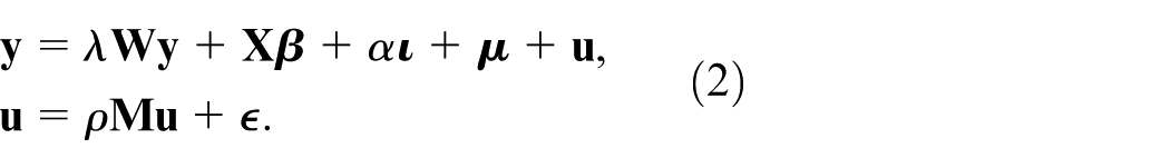
We assume the following spatial autoregressive (SAR) model with autoregressive disturbances:³

\begin{matrix} y_{t} & = λ W_{t} y_{t} + X_{t} β + α ι_{t} + μ_{t} + u_{t}, \\ u_{t} & = ρ M_{t} u_{t} + ϵ_{t}, \end{matrix}

(1)

where $t = 1, \dots, T$ denote time periods. Let the number of observations in year t be $N_{t}$ , the dependent variable $y_{t}$ in (1) is an $N_{t} \times 1$ vector of firm-level TFP estimates in year t. $W_{t}$ and $M_{t}$ are two $N_{t} \times N_{t}$ maximum row-normalised spatial weight matrices with zeros in the main diagonal. Because the number of observations varies with time, both $W_{t}$ and $M_{t}$ are time-varying. $X_{t}$ is an $N_{t} \times K$ matrix of K exogenous regressors. $ι_{t}$ is an $N_{t} \times 1$ vector of all ones. $μ_{t}$ is an $N_{t} \times 1$ vector of time-invariant individual effects. Finally, the error term $u_{t}$ is assumed to be generated by a spatial autoregressive process with i.i.d. disturbances $ϵ_{t}$ whose mean is zero and variance is $σ^{2}$ .

Stacking the equations over time periods, we can transform (1) into its panel representation:

\begin{matrix} y = λ Wy + X β + α ι + μ + u, \\ u = ρ Mu + ϵ . \end{matrix}

(2)

Here $y = {(y_{1}^{'}, y_{2}^{'}, \dots, y_{T}^{'})}^{'}$ , and other vectors (as well as $X$ ) are defined similarly. Let $N = \sum_{t = 1}^{T} N_{t}$ be the total number of observations. $W = diag (W_{1}, W_{2}, \dots, W_{T})$ is an $N \times N$ block-diagonal matrix with $W_{t}$ , $t = 1, \dots, T$ on the diagonal. $M$ is constructed in the same way.

Clearly, (2) implies:

E (u u^{'}) = σ_{ε}^{2} {(I_{N} - ρ M)}^{- 1} {(I_{N} - ρ M^{'})}^{- 1} = σ_{ε}^{2} {(I_{N} - ρ (M + M^{'}) + ρ^{2} M^{'} M)}^{- 1},

(3)

and

E ((Wy) u^{'}) = E (W {(I_{N} - λ W)}^{- 1} u u^{'}) = W {(I_{N} - λ W)}^{- 1} E (u u^{'}) \neq 0 .

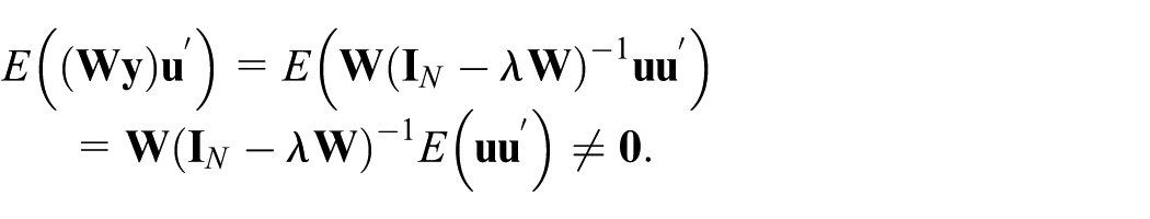
Therefore, we have both endogeneity and non-spherical disturbances. To obtain consistent estimates of the structural parameters, we can find instruments for the RHS endogenous variable $Wy$ . Before doing that, we need to swipe off the fixed effects by taking the within transformation of (2). For convenience, let us denote the matrices of within and between transformations by $Q_{0}$ and $Q_{1}$ , respectively.⁴ Note $Q_{0} μ = 0$ , we have:

Q_{0} y = λ Q_{0} Wy + Q_{0} X β + Q_{0} u .

(5)

Despite the autoregressive structure in $u$ , the error term in (5) has zero mean, and the expectation of the RHS endogenous variable $Q_{0} Wy$ turns out to be:

\begin{array}{l} E (Q_{0} W y) = Q_{0} W {(I_{N} - λ W)}^{- 1} (X β + μ + α ι) \\ = Q_{0} \sum_{k = 0} λ^{k} W^{k + 1} (X β + μ + α ι), \end{array}

(6)

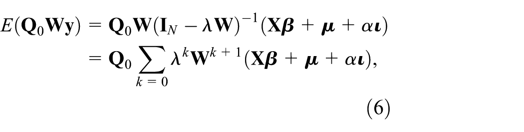
which suggests that $Q_{0} Wy$ in (5) can be instrumented by⁵:

G_{0} = (Q_{0} X, Q_{0} WX, Q_{0} W^{2} X, \dots) .

(7)

In this way, the structural parameters $δ = (λ, β^{'}, α)^{'}$ can be consistently estimated by 2SLS, which estimator we denote by ${\hat{δ}}_{W}$ .

Above is the procedure proposed by Kelejian and Prucha (1998). ${\hat{δ}}_{W}$ is consistent as far as $u$ is orthogonal to the exogenous regressors $X$ . It remains to find a proper standard error for this estimator. Let us denote $(Q_{0} Wy, Q_{0} X)$ by $Z_{0}$ and the projection matrix onto $G_{0}$ by $P_{G_{0}}$ , then:

{\hat{δ}}_{W} - δ = {(\frac{Z_{0}^{'} P_{G_{0}} Z_{0}}{N})}^{- 1} \frac{Z_{0}^{'} P_{G_{0}} u}{N},

(8)

which leads to a sandwich-type variance estimator with (3) in the middle. Clearly, the conventional HAC standard errors are incapable of modelling (3). In this study we obtain the standard errors by cluster bootstrapping, treating each individual (firm) as a cluster. Note that ${\hat{δ}}_{W}$ is simply a one-step GMM estimator assigning equal weights to the moment conditions. The two-step or the iterated GMM estimator is theoretically more efficient. Again, bootstrap standard errors are preferred in either case.

Choice of specification and issues with unbalanced panels

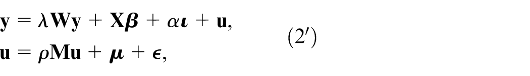
A competing model for (2) is the random-effects specification:

\begin{matrix} y & = λ Wy + X β + α ι + u, \\ u & = ρ Mu + μ + ϵ, \end{matrix}

(2′)

where the individual effects $μ$ is assumed to be uncorrelated with $X$ . The FG2SLS procedure of Kelejian and Prucha (1998) can be easily adapted to unbalanced panels under the random effects assumption. The resulting estimator ${\hat{δ}}_{R}$ is shown to be consistent but more efficient than the fixed effects estimator ${\hat{δ}}_{W}$ (Mutl and Pfaffermayr, 2011). Details of the FG2SLS procedure and the asymptotic distribution of ${\hat{δ}}_{R}$ can be found in Section B.2 of the supplementary material (available online).

Our specification of the fixed effects model (2) is different from that of the random effects model (2′). In the FG2SLS literature (e.g. Kelejian et al., 2004; Mutl and Pfaffermayr, 2011), both models are given by (2′), i.e. the individual effects enter the error component $u$ . This specification allows a similar feasible GLS transformation on the fixed effects model, resulting in a more efficient within estimator than the one obtained here ( ${\hat{δ}}_{W}$ ). The unified treatment also facilitates a subsequent Hausman test. Such advantages, however, rely heavily on the commutativity of the within and the spatial lag transformations, which is automatically satisfied if the panel is balanced and if the spatial weight matrices are time-invariant. Without commutativity, this advantage becomes an analytical burden. To see this, let’s note that the within-transformation of (2′) gives:

Q_{0} y = λ Q_{0} Wy + Q_{0} X β + Q_{0} {(I - ρ M)}^{- 1} (μ + ϵ) .

(5′)

Since $Q_{0} {(I_{N} - ρ M)}^{- 1} \neq {(I_{N} - ρ M)}^{- 1} Q_{0}$ , the individual effects $μ$ do not vanish. Under the fixed effects assumption, the error component $Q_{0} {(I - ρ M)}^{- 1} (μ + ϵ)$ is correlated with $X$ , so the within estimator becomes inconsistent.

By separating the individual effects from the error component, (2) ensures the consistency of ${\hat{δ}}_{W}$ . The change in model specification is not without a cost: the FG2SLS procedure of Kelejian and Prucha (1998) does not apply to (2) in general. This is because the estimation of $ρ$ must be based on estimates of $Q_{0} u$ , which is:

{\hat{u}}_{0} = \hat{Q_{0} u} = Q_{0} (y - \hat{λ} Wy - X \hat{β} - \hat{α} ι) .

(9)

If the spatial weights $M_{t}$ are time-invariant, the within transformation $Q_{0}$ and the spatial lag operation $M$ are commutative in (2), so that:

(I - ρ M) Q_{0} u = Q_{0} (I - ρ M) u = Q_{0} ϵ .

(10)

Thus, $(I - ρ M) \hat{Q_{0} u}$ can be used to construct the moment conditions regarding $Q_{0} ϵ$ . Without commutativity, however, (10) is invalid and $(I - ρ M) \hat{Q_{0} u}$ becomes an estimate of $(I - ρ M) Q_{0} {(I - ρ M)}^{- 1} ϵ$ , which does not lead to solvable moment conditions because of the unknown parameter $ρ$ (cf. S7).

Even if we are given a consistent estimator of $ρ$ , the time-varying spatial weights remain an obstacle to GLS estimation. To see this, let’s note that the transformed equation for (2) is:

(I - ρ M) y = λ (I - ρ M) Wy + (I - ρ M) X β + (I - ρ M) (α ι + μ) + ϵ .

(11)

If $M$ does not commute with $Q_{0}$ , the new error component $(I - ρ M) (α ι + μ) + ϵ$ is hard to deal with whether we adopt the fixed or random effects assumption.

The above discussion reveals the critical constraint imposed by unbalanced panels on the fixed effects model. In order to obtain consistent estimates of the structural parameters from least squares, one must choose (2) over (2′). By doing so, one has to forfeit the efficiency gains from the FG2SLS procedure. Nevertheless, Kelejian et al. (2004) show that such efficiency gains, if any, could be small in magnitude with even a moderate sample size.

Unbalanced panels also introduce minor changes to the FG2SLS procedure for the random effects model (2′). Because $Q_{0}$ does not commute with $M$ , the moment conditions in (S7) differ from their balanced-panel counterparts. For a similar reason, (S11) now consists of more instruments.

The fixed effects estimator ${\hat{δ}}_{W}$ , which we develop for (2) is also consistent in (2′) under the random effects assumption $E (μ | X) = 0$ . In the latter case, ${\hat{δ}}_{R}$ is consistent but more efficient.⁶ However, if the random effects assumption is rejected, we shall estimate ${\hat{δ}}_{W}$ with (2).

Data description and measurement

We obtain firm-level data from the China Industry Survey conducted by the National Bureau of Statistics. The data set was issued on an annual basis from 1996 through 2010, covering over 160,000 establishments (firms) in most years.⁷ The accounting and financial variables permit us to estimate firm-level productivity and construct proxies for firm characteristics. The data set also provides locational information for each firm. Because of its wide coverage and comprehensive information, this unique data set has been widely used in empirical studies on China’s manufacturing sector, especially those on productivity analysis (Baltagi et al., 2015; Brandt et al., 2012; Hu et al., 2015).

The basic geographic unit in this study is an (urban) district or county, defined by the Codebook of Administrative Divisions (National Standard GB/T 2260).⁸ Using the administrative codes, the location of each firm is identified as the district/county in which it operates, but we have no further geographic information within the district/county. We acquire a shape file for all county-level jurisdictions from a commercial source. The shape file enables us to construct spatial neighbourhood relations among jurisdictions either by contiguity or by spatial distance between administrative centres.

Our study also employs data on the budgetary expenditure of local governments at the district/county level. The data are extracted from the Fiscal Statistics of Cities and Counties (various issues) compiled by the Ministry of Finance. They are then merged into the main data set by matching administrative codes. Details of our data preparation process can be found in Section A of the supplementary material (available online).

After these steps, we are able to assemble a longitudinal data set of 615,624 distinct firms from 470 four-digit industries, located in 2862 districts/counties. The data set provides a near-complete coverage of China’s above-scale industrial firms over 1999–2007.⁹ We observe a remarkable amount of entrants and exits each year, resulting in a highly unbalanced panel.

In this study, we focus on the electric apparatus industry (industry code 3900) over the period of 1999–2007. The choice of this industry is based on the following concerns: first, the industry is technology intensive, thus we expect technological spillovers to be more pronounced; second, this industry provides a large sample size (over 99,000), with over 27,000 firms located in 1629 districts/counties. The wide spatial coverage allows us to conduct spatial analysis without heavy data loss. The spatial distributions of firms and employment in this industry are shown by Figure 1 and Figure S1 (in supplementary material, available online). A pattern of agglomeration is evident in these graphs. Firms and employment cluster in the eastern coast and inland industrial centres, while the vast areas in the west are unoccupied. This observation suggests a strong spatial linkage in the locational choice of firms, and likely spatial interactions between firms when they are close.

Figure 1.

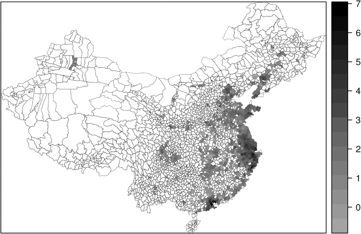
District/county subtotal: number of firms in the electric apparatus industry, 2005–2007 average.

As previously explained, each firm is pinpointed to a district/county. In this regard, a firm has two types of neighbours: those in the same jurisdiction (intra-regional) and those in neighbouring jurisdictions (inter-regional). Thus, we introduce two spatial weight matrices to the SAR model (1):

W_{1 t} y_{ikt} = \sum_{\binom{j \in I_{t} (k)}{j \neq i}} l_{jkt} y_{jkt} / \sum_{\binom{j \in I_{t} (k)}{j \neq i}} l_{jkt},

(12)

W_{2 t} y_{ikt} = \sum_{\binom{j \in I_{t} (k^{'})}{k^{'} \in N (k)}} l_{j k^{'} t} y_{j k^{'} t} / \sum_{\binom{j \in I_{t} (k^{'})}{k^{'} \in N (k)}} l_{j k^{'} t} .

(13)

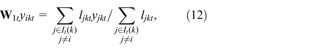
Here the subscripts $i$ and j denote firms, k and $k^{'}$ denote jurisdictions, and t denotes time. $I_{t} (k)$ is the set of all firms located in jurisdiction k in year t, and $N (k)$ is the set of all neighbouring jurisdictions of k. y is any variable to be weighted, and $l_{ikt}$ is the employment of firm i in jurisdiction k and year t. The construction is based on the premise that larger firms (measured by employment) exert stronger influence on their neighbours than smaller ones. Contiguous (Rook style) jurisdictions are treated as neighbours.

Both $W_{1 t}$ and $W_{2 t}$ are maximum row normalised, and they have zeros in the main diagonal. For simplicity, we use a single spatial lag in the error component of (2′), i.e. we assume $u = ρ W_{1} u + μ + ϵ$ .

The SAR model (1) considers two types of exogenous variables: firm characteristics and local market conditions. With individual fixed effects, however, the model allows time-varying factors only. R&D (rd) and export (ex) activities are respectively measured by the share of new products in gross output and the share of exports in gross sales. We consider four aspects of the local market environment: localisation economies (spec), industrial employment density (dsty), competition (comp), and public expenditure (pub). spec is defined as the location quotient of industry 3900 in the jurisdiction (cf. Glaeser et al., 1992), and dsty is defined as the ratio of total industrial employment to the surface area of the jurisdiction (log-transformed). Following Combes et al. (2004), we define comp as the Herfindahl-Hirschman index of employment concentration in the jurisdiction-industry:¹⁰

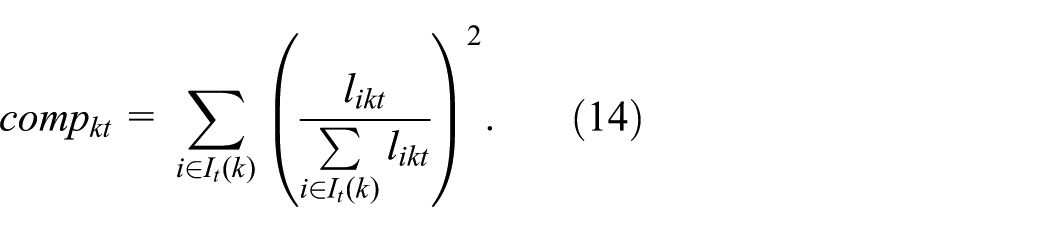
com p_{kt} = \sum_{i \in I_{t} (k)} {(\frac{l_{ikt}}{\sum_{i \in I_{t} (k)} l_{ikt}})}^{2} .

(14)

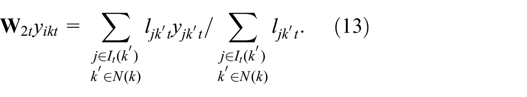
The HHI takes values between zero and unity. Finally, $pub$ is measured by the total budgetary expenditure in the jurisdiction (log-transformed).¹¹

We adopt the modelling strategy of Yu et al. (2013) and allow market conditions to influence firms in neighbouring jurisdictions. Therefore, their spatial lags $W_{2 t} spe c_{kt}$ , $W_{2 t} dst y_{kt}$ , $W_{2 t} com p_{kt}$ , and $W_{2 t} pu b_{kt}$ are also included as regressors. In summary, we end up with the following empirical model:

\begin{matrix} tf p_{ikt} = λ_{1} W_{1 t} tf p_{ikt} + λ_{2} W_{2 t} tf p_{ikt} + β_{1} r d_{ikt} \\ + β_{2} e x_{ikt} + β_{3} spe c_{kt} + β_{4} dst y_{kt} + β_{5} com p_{kt} \\ + β_{6} pu b_{kt} + β_{7} W_{2 t} spe c_{kt} + β_{8} W_{2 t} dst y_{kt} \\ + β_{9} W_{2 t} com p_{kt} + β_{10} W_{2 t} pu b_{kt} + α + error term, \end{matrix}

(15)

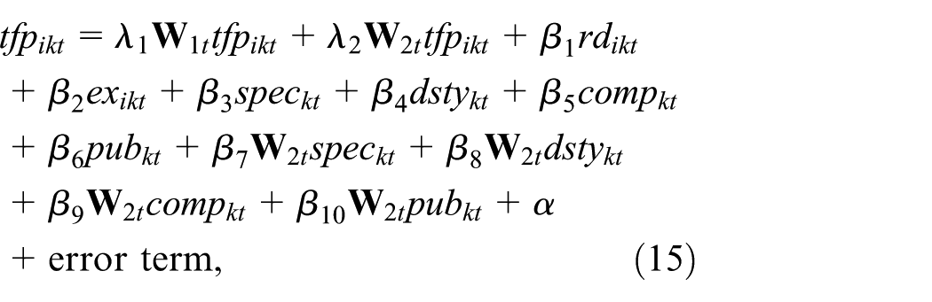
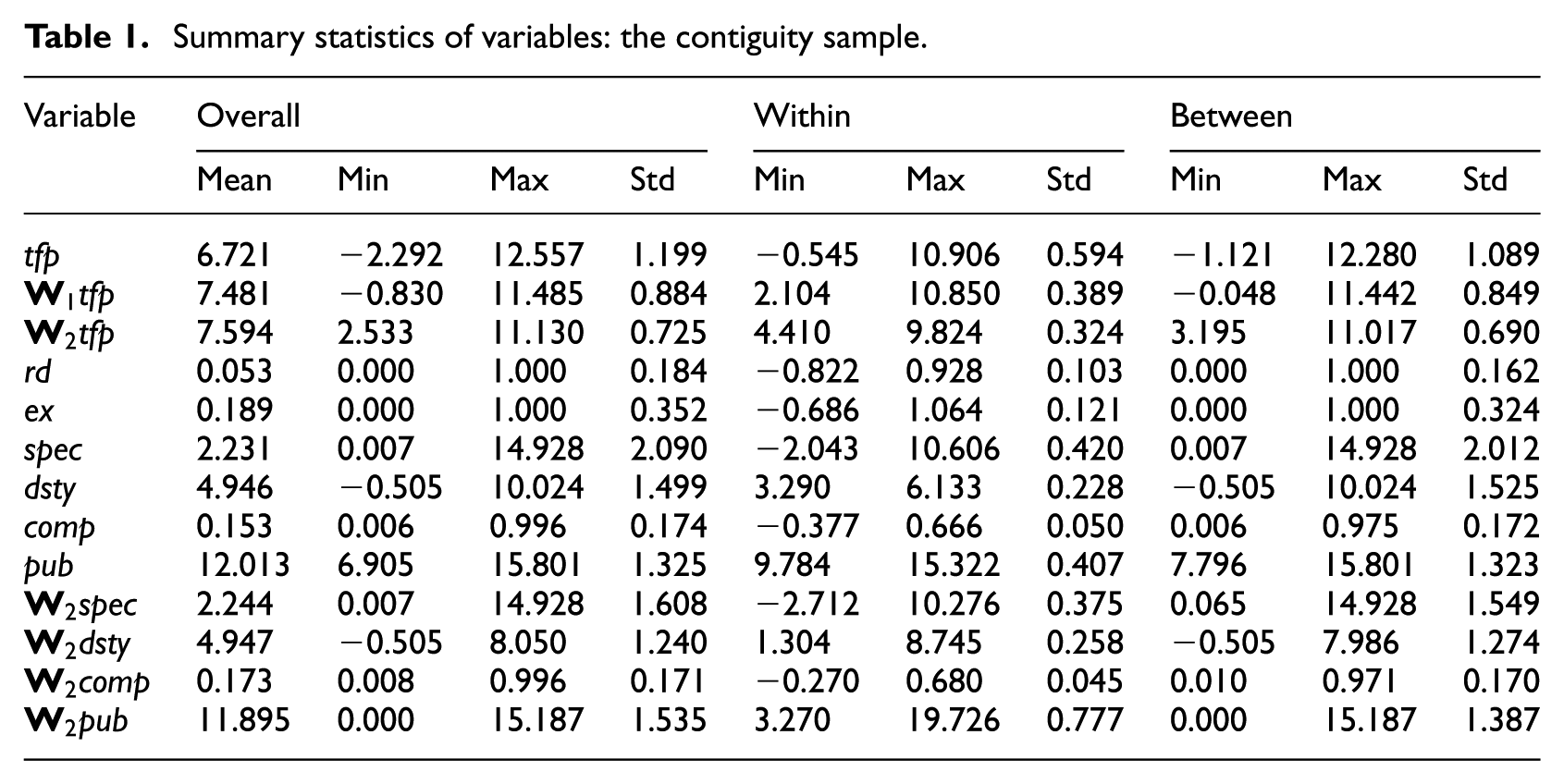
where the error term can be either $μ + {(I - ρ W_{1})}^{- 1} ϵ$ in the fixed effects model or ${(I - ρ W_{1})}^{- 1} (μ + ϵ)$ in the random effects model.

In practice, we retain the observations that have both types of neighbours, then those with complete observations. This leaves us with a sample size of 84,727 (26,174 firms). The descriptive statistics are summarised in Table 1. The statistics reveal substantial within-group variations in rd, ex, tfp and the spatial lags of tfp. But for local market condition variables as well as their spatial lags, the between-group variations dominate.

Table 1.

Summary statistics of variables: the contiguity sample.

Variable	Overall				Within			Between
Variable	Mean	Min	Max	Std	Min	Max	Std	Min	Max	Std
tfp	6.721	−2.292	12.557	1.199	−0.545	10.906	0.594	−1.121	12.280	1.089
$W_{1} tfp$	7.481	−0.830	11.485	0.884	2.104	10.850	0.389	−0.048	11.442	0.849
$W_{2} tfp$	7.594	2.533	11.130	0.725	4.410	9.824	0.324	3.195	11.017	0.690
rd	0.053	0.000	1.000	0.184	−0.822	0.928	0.103	0.000	1.000	0.162
ex	0.189	0.000	1.000	0.352	−0.686	1.064	0.121	0.000	1.000	0.324
spec	2.231	0.007	14.928	2.090	−2.043	10.606	0.420	0.007	14.928	2.012
dsty	4.946	−0.505	10.024	1.499	3.290	6.133	0.228	−0.505	10.024	1.525
comp	0.153	0.006	0.996	0.174	−0.377	0.666	0.050	0.006	0.975	0.172
pub	12.013	6.905	15.801	1.325	9.784	15.322	0.407	7.796	15.801	1.323
$W_{2} spec$	2.244	0.007	14.928	1.608	−2.712	10.276	0.375	0.065	14.928	1.549
$W_{2} dsty$	4.947	−0.505	8.050	1.240	1.304	8.745	0.258	−0.505	7.986	1.274
$W_{2} comp$	0.173	0.008	0.996	0.171	−0.270	0.680	0.045	0.010	0.971	0.170
$W_{2} pub$	11.895	0.000	15.187	1.535	3.270	19.726	0.777	0.000	15.187	1.387

Empirical results

The baseline model

Table 3 summarises the estimates of the baseline model (15). We first report the conventional fixed effects estimates in column 1 as the benchmark. Column 2 reports the fixed effects 2SLS estimator discussed in section ‘The spatial fixed effects model’. Since we have included two spatial lags in (15), the list of instruments in (7) has to be expanded.¹² To account for the potential spatial correlation as well as heteroscedasticity in the error terms, the standard errors reported here are obtained from 50 bootstrap samples of firms. In column 3, we implement the conventional two-step GMM using the same set of instruments. The same bootstrapping strategy is used to obtain the standard errors. Finally, we report the FG2SLS estimates of the random effects model in column 4.¹³ Because the error terms in the transformed structural equation (S9) are spherical, we report the conventional standard errors in column 4.

The estimates in column 2 are notably different from those in column 1, indicating endogeneity bias in the latter. Despite its theoretical advantage in efficiency, the two-step GMM procedure (column 3) yields highly similar estimates and virtually identical standard errors. We prefer the 2SLS estimator because it is easier to implement.¹⁴ The empirical evidence is clearly against the random effects specification when we compare columns 2 and 4. First, the two sets of estimates are sizably different, especially the parameters of interest ( ${\hat{λ}}_{1}$ and ${\hat{λ}}_{2}$ ). Because ${\hat{δ}}_{W}$ is always consistent, this observation suggests that ${\hat{δ}}_{R}$ is not. Second, the estimated idiosyncrasies $\hat{μ}$ in (2) is strongly correlated with $X$ : $cor (\hat{μ}, X {\hat{β}}_{W}) = - 0.489$ . The standard error of $\hat{μ}$ (1.225) is large relative to that of $\hat{Q_{0} u}$ (0.669). Thus we have a strong case for the fixed effects assumption $E (μ | X) \neq 0$ .¹⁵ Based on these observations, we choose the fixed effects model and base our subsequent inferences on column 2.

According to these estimates, firm-level TFP increases by 3.6% if that of intra-regional neighbours increases uniformly by 10%. The estimated spatial AR coefficient ${\hat{λ}}_{1}$ is comparable with that of Baltagi et al. (2015).¹⁶ ${\hat{λ}}_{2}$ , which measures the inter-regional spillover effect, is much smaller in size and insignificant. Our results demonstrate that technology spillovers occur locally, but attenuate rapidly in spatial distance. Intuitively, any benefits from technology enhancement via diffusing mechanisms would be received first by close neighbours because of geographic proximity, before diffusing to more distant neighbours through imitation, labour mobility, and input-output linkage.

The coefficients on rd and ex are both highly significant. A 10% increase in R&D and export activities results in a 1.7% and a 0.9% increase in productivity, respectively.¹⁷ These results are qualitatively in line with the empirical findings in China. Among the agglomeration variables, localisation (spec) has little effect on firm productivity, but those of employment density (dsty) and competition (comp) are strong and positive.¹⁸ A 10% increase in employment density results a 1.8% productivity gain by local firms. If HHI decreases by ten percentage points, which could be the the result of splitting five equal-sized firms into ten, the productivity of local firms will increase by 7.6%. We also observe productivity gains from public expenditures. A 10% increase in local public expenditure increases productivity by 1.0%. The spatial lags of all market condition variables have qualitatively the same, but much weaker effects than the unlagged variables. Thus we find evidence that local market conditions ‘spillover’ into neighbouring jurisdictions in the sense of Rosenthal and Strange (2003, 2008).

To summarise, our baseline model identifies strong and significant technological spillovers within jurisdictions. It also shows that the spillovers become much weaker and insignificant when the spatial linkage is extended to include firms in neighbouring jurisdictions. Next, we extend the baseline model to study whether and how geography-related or socioeconomic factors may influence the strength of technological spillovers.

Geography, administrative division, and border effect

The first geographic factor coming to mind is spatial distance. By definition, the inter-regional neighbours are more distant than the intra-regional ones because the former are located in different, albeit contiguous jurisdictions. The inter-regional spillover effect (measured by $λ_{2}$ ) is weaker than the intra-regional one (measured by $λ_{1}$ ) because interactions among firms dissipate with distance. In the same logic, if some firms are more distant from their inter-regional neighbours than others, we expect them to interact more with intra-regional neighbours but less with inter-regional neighbours. Consequently, $λ_{1}$ should be larger and $λ_{2}$ smaller for these firms. Even though we cannot precisely measure the bilateral distance between firms, we can proxy the distance from inter-regional neighbours by the surface area of a jurisdiction: firms located in large jurisdictions must be more distant from the border, hence inter-regional neighbours.

A second geographic factor is China’s administrative division. For historical reasons, urban districts and counties are assigned different roles in the administrative hierarchy. Urban districts form the administrative and economic centre of the prefecture. They also serve as the transportation hub of the region. Because urban districts have tight linkages with the rest of the prefecture, we expect firms in urban districts to interact more with their inter-regional neighbours, e.g. $λ_{1}$ should be smaller and $λ_{2}$ larger for these firms.

Geography may also affect the spillover effects through the border effect.¹⁹ It has long been known that China’s domestic market is highly segregated, partly because of local protectionism (Bai et al., 2008; Poncet, 2005). Inter-jurisdictional barriers are likely to hinder inter-regional spillovers across the prefecture border. Besides, districts/counties within the same prefecture are all subject to the economic plans (typically the so-called Five-Year Plans) made by the prefecture government. They share a higher level of similarity in institutional arrangement and economic development than jurisdictions belonging to different prefectures. The resulting home bias (cf. Head and Mayer, 2000) may also discourage economic relations across the prefecture border. For these reasons, we postulate that the inter-regional spillover effect is weakened by prefecture borders. Other things being equal, if more inter-regional neighbours of a firm are across the prefecture border, we expect a larger $λ_{1}$ and a smaller $λ_{2}$ for this firm.

To test the first two hypotheses, we construct dummy variables large and county to identify the large jurisdictions and non-urban districts.²⁰ Measuring the (prefecture) border effect needs more work. For each jurisdiction, we first identify its neighbouring jurisdictions, including those across the prefecture border. We then define border as the ratio of industrial employment in cross-border neighbours to that of all neighbouring jurisdictions. A large value means that the prefecture border is sharply felt by firms in the jurisdiction. These variables are then interacted with $W_{1} tfp$ and $W_{2} tfp$ . According to the reasonings above, we expect a positive sign on the first interaction term and a negative sign on the second one. Table 2 presents the summary statistics of these variables. Clearly, firms in the electric apparatus industry sort into urban districts (65.1%) and/or small-sized jurisdictions (71.6%). Judged by the sample mean, a substantial fraction (39.3%) of industrial employment in neighbouring jurisdictions are across the prefecture border.

Table 2.

Summary statistics of interacting factors.

Variable^a	National^b				The contiguity sample^c
Variable^a	Mean	Min	Max	Std	Mean	Min	Max	Std
large	0.500	0.000	1.000	0.500	0.284	0.000	1.000	0.451
county	0.705	0.000	1.000	0.456	0.349	0.000	1.000	0.477
border	0.368	0.000	1.000	0.304	0.393	0.000	1.000	0.348
tran	0.776	0.007	31.94	1.603	2.409	0.034	15.08	2.572
hwy	0.709	0.004	28.52	1.464	2.150	0.031	15.07	2.512
rail	0.045	0.000	1.021	0.092	0.191	0.000	1.021	0.247
tel	0.219	0.021	2.993	0.197	0.528	0.021	2.993	0.466
fdi	0.157	0.000	0.938	0.177	0.361	0.000	0.938	0.225
fdi1	0.087	0.000	2.710	0.151	0.176	0.000	2.710	0.202
fin	3.377	0.927	19.85	1.119	3.976	0.927	10.83	1.541
uti	3.187	0.075	46.32	1.647	2.199	0.646	8.419	0.939
edu	0.887	0.000	11.02	1.390	1.971	0.000	11.02	1.906

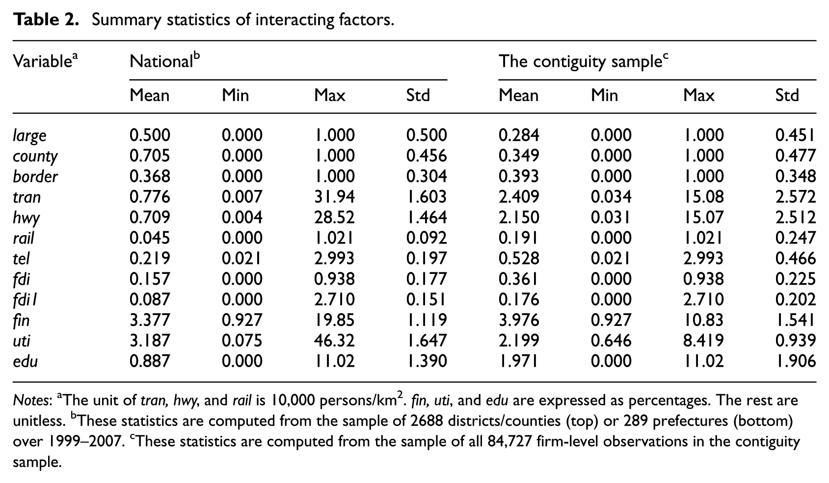
Notes: ^aThe unit of tran, hwy, and rail is 10,000 persons/km². fin, uti, and edu are expressed as percentages. The rest are unitless. ^bThese statistics are computed from the sample of 2688 districts/counties (top) or 289 prefectures (bottom) over 1999–2007. ^cThese statistics are computed from the sample of all 84,727 firm-level observations in the contiguity sample.

In Table 4, we extend the baseline model to include the interaction terms. In all specifications, we use the full set of controls as we did in Table 3. All models are regressed by FE-2SLS and the standard errors are obtained from 50 bootstrap repetitions.²¹

Table 3.

The baseline model: the contiguity sample ( $N = 84, 727$ ).

Dependent variable: tfp
Regressor	1	2	3	4
Regressor	FE^a	FE-2SLS^b	FE-GMM^b	RE-FG2SLS
$W_{1} tfp$	0.19*	0.355**	0.358**	0.674**
	(0.011)	(0.076)	(0.076)	(0.009)
$W_{2} tfp$	0.169**	0.095	0.099	0.127**
	(0.013)	(0.085)	(0.082)	(0.009)
rd	0.167**	0.175**	0.169**	0.404**
	(0.027)	(0.030)	(0.029)	(0.016)
ex	0.08*	0.086**	0.085**	0.071**
	(0.025)	(0.028)	(0.028)	(0.009)
spec	0.029**	0.007	0.008	−0.01*
	(0.009)	(0.014)	(0.014)	(0.002)
dsty	0.214**	0.178**	0.167**	−0.009**
	(0.022)	(0.025)	(0.026)	(0.002)
comp	−0.601**	−0.757**	−0.777**	0.124**
	(0.075)	(0.123)	(0.122)	(0.016)
pub	0.129**	0.097**	0.096**	0.002
	(0.011)	(0.022)	(0.022)	(0.003)
$W_{2} spec$	−0.026**	−0.013	−0.011	−0.033**
	(0.009)	(0.012)	(0.012)	(0.002)
$W_{2} dsty$	0.041**	0.055**	0.064**	−0.026**
	(0.017)	(0.015)	(0.017)	(0.003)
$W_{2} comp$	−0.598**	−0.438**	−0.414**	0.019
	(0.078)	(0.121)	(0.118)	(0.019)
$W_{2} pub$	0.019**	0.014**	0.014**	0.002
	(0.005)	(0.006)	(0.005)	(0.002)
Intercept	1.134**	1.029**	1.010**	1.293**
	(0.145)	(0.176)	(0.175)	(0.040)
$R^{2}$	0.133	0.126	–	0.732
${\hat{σ}}_{μ}$	1.243	1.225	–	1.353
${\hat{σ}}_{u}$ ( ${\hat{σ}}_{ϵ}$ )^c	0.666	0.669	–	0.561
$\hat{ρ}$	–	–	–	−0.957

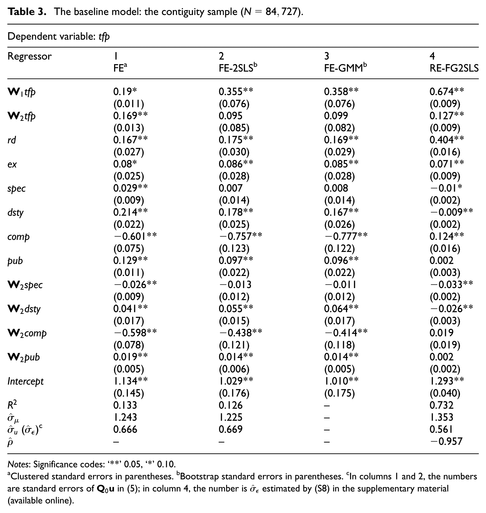
Notes: Significance codes: ‘**’ 0.05, ‘*’ 0.10.

Clustered standard errors in parentheses. ^bBootstrap standard errors in parentheses. ^cIn columns 1 and 2, the numbers are standard errors of $Q_{0} u$ in (5); in column 4, the number is ${\hat{σ}}_{ϵ}$ estimated by (S8) in the supplementary material (available online).

Table 4.

Impact of geography-related factors on spillover effects: the contiguity sample ( $N = 84, 727$ ).

Dependent variable: tfp¹
Regressor	1	2	3	4	5	6	7
$W_{1} tfp$	0.333**	0.295**	0.348**	0.280**	0.346**	0.285**	0.276**
	(0.076)	(0.069)	(0.078)	(0.071)	(0.078)	(0.070)	(0.074)
$W_{2} tfp$	0.111	0.121*	0.065	0.160**	0.110	0.117*	0.153**
	(0.083)	(0.070)	(0.070)	(0.075)	(0.076)	(0.066)	(0.074)
interactions:
$W_{1} tfp \times large$	0.326**	–	–	0.436**	0.284**	–	0.309**
	(0.074)			(0.086)	(0.067)		(0.077)
$W_{2} tfp \times large$	−0.203**	–	–	−0.364**	−0.139**	–	−0.219**
	(0.078)			(0.095)	(0.069)		(0.082)
$W_{1} tfp \times county$	–	0.265**	–	−0.027	–	0.184**	0.034
		(0.060)		(0.069)		(0.058)	(0.068)
$W_{2} tfp \times county$	–	−0.070	–	0.21*	–	0.014	0.159**
		(0.064)		(0.083)		(0.065)	(0.081)
$W_{1} tfp \times border$	–	–	0.215**	–	0.086	0.236**	0.126
			(0.097)		(0.094)	(0.097)	(0.091)
$W_{2} tfp \times border$	–	–	−0.247**	–	−0.178*	−0.306**	−0.240**
			(0.097)		(0.092)	(0.101)	(0.090)
Further controls	Yes	Yes	Yes	Yes	Yes	Yes	Yes
$R^{2}$	0.121	0.124	0.119	0.123	0.118	0.120	0.123
${\hat{σ}}_{μ}$	1.279	1.258	1.253	1.288	1.333	1.283	1.340
${\hat{σ}}_{u}$	0.670	0.669	0.671	0.670	0.672	0.671	0.670

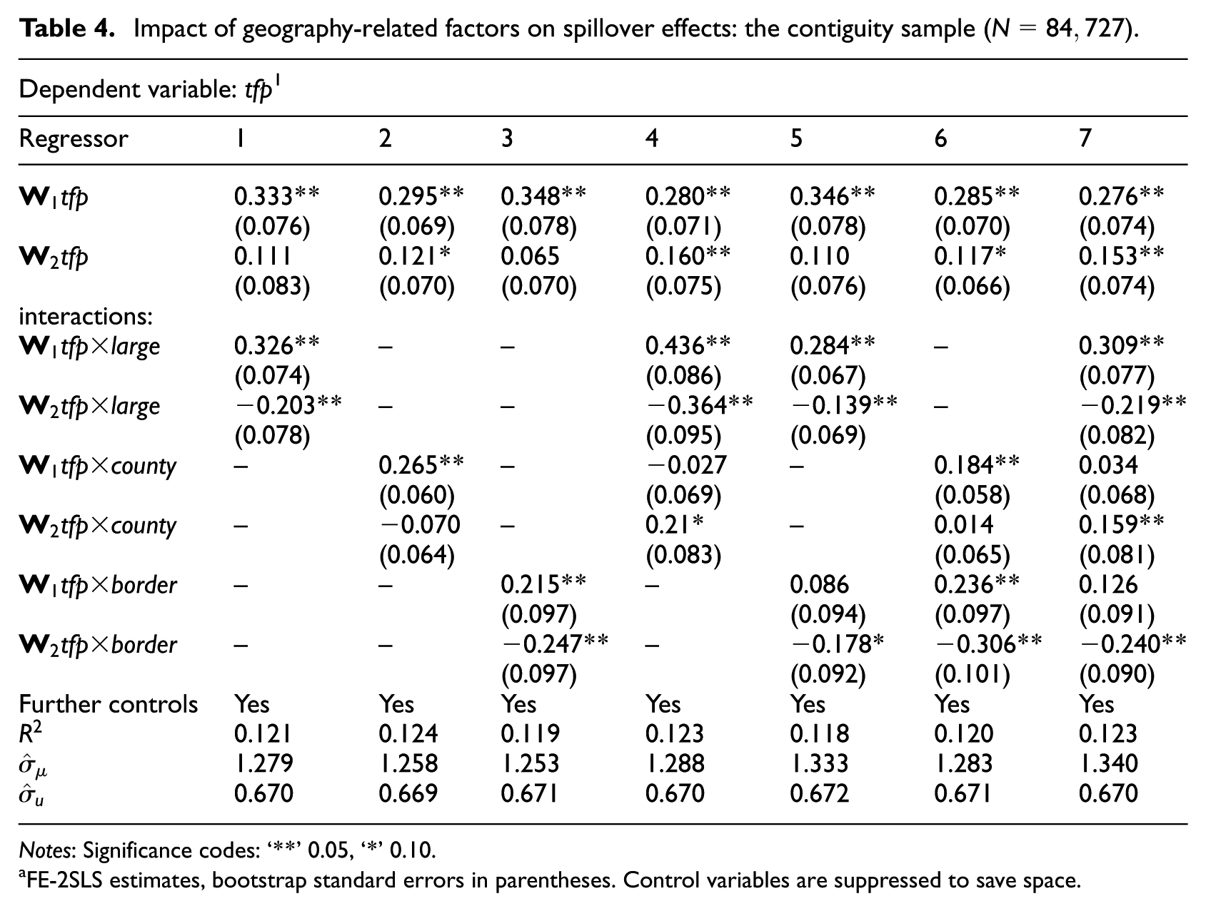
Notes: Significance codes: ‘**’ 0.05, ‘*’ 0.10.

FE-2SLS estimates, bootstrap standard errors in parentheses. Control variables are suppressed to save space.

When large, county, and border are introduced one at a time (columns 1–3), they do deliver the expected outcomes: the interaction with $W_{1} tfp$ has a positive sign, that with $W_{2} tfp$ has a negative sign, and both coefficients are significant, $W_{2} tfp \times county$ being the only exception. These results thus support all three hypotheses. When multiple factors are introduced together, the results on large are qualitatively the same as before. The coefficients of $W_{1} tfp \times border$ and $W_{2} tfp \times border$ are generally less significant but they still have the expected signs. county gives unexpected outcomes when other factors are present. For twice the coefficient of $W_{1} tfp \times county$ becomes quite small and insignificant, while that of $W_{2} tfp \times county$ is significant but with the wrong sign (columns 4 and 7). Correlations among these factors may explain the poor performance of county when other factors are present.²² Meanwhile, the structural parameters of all controls (including the spatial lags of market condition variables) are highly robust to the specifications tried here. We observe little change to the empirical estimates throughout.

Infrastructure, FDI, industrial service, and education

Transport cost is central to agglomeration theories. Distance inhibits spillovers because it increases the transport cost for goods, people, and ideas. Transport infrastructure reduces the cost of shipping goods and moving people. Similarly, advancements in information and communication technology (ICT) have substantially reduced the cost of transmitting information over distance. Hence, both types of infrastructure make distance less important and foster inter-regional spillovers (Yilmaz et al., 2002; Yu et al., 2013).²³ Thus, we postulate that they amplify the inter-regional spillover effect (larger $λ_{2}$ ) but make the intra-regional spillover effect less important (smaller $λ_{1}$ ).²⁴

There is extensive literature on the role of FDI in China’s manufacturing. They are found to generate positive technological spillovers to neighbouring firms (Tanaka and Hashiguchi, 2012; Xu and Sheng, 2012). Therefore, we also study whether the presence of FDI affect the intra- and inter-regional spillover effects through $λ_{1}$ and $λ_{2}$ . Other regional factors affecting the spillover effects include the business service sector (Ke et al., 2014) and human capital (Moretti, 2004).

In what follows we investigate the effects of these factors on $λ_{1}$ and $λ_{2}$ . These factors are measured using annual prefecture-level data from the China City Statistical Yearbook, 2000–2008. We use the density (divided by the surface area of the prefecture) of passenger traffic by all transport modes (tran), highway (hwy), and railway (rail) to measure the capacity of transport facilities.²⁵ The yearbook provides the number of subscribers to multiple telecommunication services, including landline phone, cellular phone, and (dial-up or broadband) internet service. We use the number of landline phone subscribers (tel) because it is the only variable available throughout the period of study. This number is divided by local population to reflect ICT penetration. We introduce two proxies for FDI intensity. fdi is defined as the share of international (including Hong Kong, Macao, and Taiwan) joint ventures in total industrial output, and fdi1 is defined as the ratio of FDI inflows to total fixed asset investment.²⁶ The size of the financial sector (fin) or the utility service sector (uti) is respectively measured by their employment shares. Finally, the level of human capital (edu) is measured by the ratio of enrolled college students to local population. Their descriptive statistics are summarised in Table 2. The statistics demonstrate large variations across the nation. The sample means suggest that firms sort into regions with better infrastructure, more FDI, and more human capital.

We interact each factor with $W_{1} tfp$ and $W_{2} tfp$ and add them to the baseline model. The model is then regressed by FE-2SLS using the instrumenting strategy described in footnote 21. Practically, each factor x is centred ( ${\tilde{x}}_{it} = x_{it} - \bar{x ¯}$ ) before entering the interaction terms so that $λ_{1}$ and $λ_{2}$ are evaluated in a region where x is at its sample mean. As usual, we obtain the standard errors from 50 bootstrap samples. Table 5 presents the results.

Table 5.

Impact of socio-economic factors on spillover effects: the contiguity sample.

Dependent variable: tfp^a
regressor	1	2	3	4	5	6	7	8	9
$W_{1} tfp$	0.329**	0.315**	0.376**	0.453**	0.339**	0.310**	0.370**	0.384**	0.400**
	(0.058)	(0.056)	(0.070)	(0.060)	(0.065)	(0.062)	(0.054)	(0.048)	(0.058)
$W_{2} tfp$	0.103**	0.109**	0.100	−0.057	0.037	0.148**	0.126*	0.063	0.039
	(0.051)	(0.048)	(0.070)	(0.048)	(0.050)	(0.051)	(0.065)	(0.053)	(0.064)
Interacting factor	tran	hwy	rail	tel	fdi	fdi1	fin	uti	edu
$W_{1} tfp \times factor$	−0.031**	−0.03*	−0.188	−0.119*	−0.085	−0.210**	0.008	0.015	−0.010
	(0.014)	(0.013)	(0.123)	(0.071)	(0.114)	(0.057)	(0.010)	(0.013)	(0.009)
$W_{2} tfp \times factor$	0.035*	0.044**	−0.24	0.128**	−0.337**	−0.526**	0.030**	0.036**	0.023**
	(0.020)	(0.020)	(0.147)	(0.042)	(0.147)	(0.096)	(0.012)	(0.017)	(0.010)
Further controls	Yes	Yes	Yes	Yes	Yes	Yes	Yes	Yes	Yes
N	84,082	84,082	74,952	84,082	84,001	83,991	84,083	84,083	83,989
$R^{2}$	0.123	0.124	0.114	0.106	0.127	0.131	0.125	0.122	0.121
${\hat{σ}}_{μ}$	1.230	1.231	1.236	1.231	1.264	1.229	1.209	1.227	1.233
${\hat{σ}}_{u}$	0.670	0.669	0.681	0.676	0.669	0.667	0.669	0.670	0.671

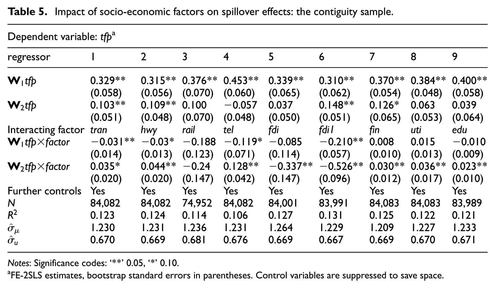
Notes: Significance codes: ‘**’ 0.05, ‘*’ 0.10.

FE-2SLS estimates, bootstrap standard errors in parentheses. Control variables are suppressed to save space.

We first observe that ${\hat{λ}}_{1}$ and ${\hat{λ}}_{2}$ are similar to those of the baseline model (column 2 of Table 3) except for the large deviations in column 4. This is what we expect from the centring strategy. Estimates of the control variables (not reported) are all fairly robust to the specifications, and the statistical inferences remain unchanged. Column 2 gives clear evidence that better highway infrastructure stimulates inter-regional spillovers. The evidence is weaker when we consider all-transport infrastructure (column 1), partly because railway infrastructure is negatively correlated with both spillover effects (column 3). The results thus suggest that inter-regional spillovers largely benefit from road transport, but not railway. Consistent with our hypothesis, telephone infrastructure is found to contribute positively to inter-regional spillovers (column 4).

We have surprising results on the role of FDI. The results from both measures (columns 5 and 6) indicate that the presence of international joint ventures hinders technological spillovers in short and long distances. Such an effect is more pronounced with fdi1. These results seem to contradict those of other researchers. The paradox arises because our definition of technological spillover is conceptually different from theirs. Precisely, Xu and Sheng (2012) and Tanaka and Hashiguchi (2012) demonstrate that higher FDI shares in the local and neighbouring regions make local firms more productive.²⁷ Note that fdi and fdi1 are respectively used as the additional regressor when we introduce the interaction terms (cf. endnote 21), the traditional view of FDI spillover (local effects only) can be tested with the coefficient of fdi or fdi1. In both regressions, the coefficient is indeed positive and highly significant, confirming the findings of Xu and Sheng (2012) and Tanaka and Hashiguchi (2012).²⁸ In contrast to their empirical strategy, we measure spillover effects by the spatial dependence of firm-level productivity ( $λ_{1}$ and $λ_{2}$ ). Therefore, we have provided new evidence that the presence of FDI firms reduces the horizontal connections among neighbouring firms, despite the fact that they bring overall productivity gains.

Employment in the financial (column 7) and utility service (column 8) sectors are found to contribute to inter-regional spillovers. Human capital (column 9) has a similar effect. But these effect are only significant on $λ_{2}$ .

Robustness checks

In this section, we repeat the spatial analysis with an alternative definition of neighbourhood relationship that is based on spatial distance. Two jurisdictions are regarded as neighbours if their administrative centres are within 50 km in great circle distance; for each firm, all other firms in neighbouring jurisdictions are treated as its inter-regional neighbours.²⁹ The spatial weight matrix $W_{2 t}$ in (15) is updated accordingly. After dropping islands and then incomplete observations, we end up with 81,331 observations (24,903 firms) for the baseline model.

Table S2 in the supplementary material (available online) presents estimates of the baseline model. There, the FE-2SLS method yields similar estimates to those in Table 3, except for $W_{2} dsty$ , which becomes insignificant. The random effects model (column 4) continues to generate very different estimates, and the empirical correlation between the individual effects and the controls remains strong: $cor (\hat{μ}, X {\hat{β}}_{W}) = - 0.502$ . Therefore, the fixed effects model is again chosen.³⁰

Table S3 re-investigates the geography-related factors. The distance-based neighbourhood relationship lends support to the hypotheses on surface area and administration type. In all specifications, the coefficients of $W_{1} tfp \times large$ , $W_{1} tfp \times county$ , $W_{2} tfp \times large$ , and $W_{2} tfp \times county$ have the expected signs; the former two are usually highly significant. However, the estimated coefficients of $W_{1} tfp \times border$ and $W_{2} tfp \times border$ are much smaller than previously estimated (Table 4), both insignificant. The previous finding regarding the prefecture border effect seems to be sensitive to the definition of inter-regional neighbours.

In Table S4 (available online), the previous results on infrastructure variables are quite robust. It is clear that inter-regional spillovers benefit strongly from overall transport infrastructure and highways; their marginal impacts on $λ_{1}$ and $λ_{2}$ are noticeably larger than previously estimated (Table 5). The effects of rail and tel are also qualitatively similar to earlier findings. The two FDI variables continue to hinder spillovers at short and long distances. In both cases, fdi1 gives clearer results. fin and edu generate almost the same estimates as the previous ones. Overall, the current results are consistent with previous ones except for (uti), whose interaction terms become insignificant.

Concluding remarks

This article studies the intra- and inter-regional technological spillovers using a panel of 26,174 firms in China’s electric apparatus industry over the period of 1999–2007. The spillover effects are measured by the spatial dependence of firm-level TFP among intra- and inter-regional neighbours. The SAR model explicitly addresses the spatial scope with two spatial AR terms. It controls for firm characteristics as well as local market conditions. The conventional spillover effects of market conditions (Rosenthal and Strange, 2003; Yu et al., 2013) are also incorporated. Later, the baseline model is extended with interaction terms to assess the impact of geographic and socio-economic factors on the spillover effects.

Empirically, we find that the intra-regional technological spillovers are stronger and more significant than the inter-regional ones. Productivity gains from local market conditions are also larger in size than from neighbouring regions. Factors that facilitate inter-regional economic connections are found to contribute positively to inter-regional spillovers and/or negatively to intra-regional spillovers. Most of the empirical results are robust to the alternative definition of inter-regional neighbours.

The current study leaves some unanswered questions that can be addressed by future research. First, we find that presence of FDI results in a lower level of spatial dependence in firm productivity. At the same time, we also observe significant productivity gains on local firms. Admittedly, the current measures of FDI are based on prefecture aggregates, which do not reflect industry or regional heterogeneity. Better measures and/or alternative empirical methods may provide insights into the mechanisms behind this phenomenon. Second, even though we study the spatial scope of spillover effects, they are both within the same industry. The literature also underpins inter-industry synergy effects through the upstream-downstream linkage (Combes and Gobillon, 2015; Rosenthal and Strange, 2004). An extension of the current model that allows inter-industry spillovers may utilise the input–output relationship among China’s industries (Hu et al., 2015; Smarzynska Javorcik, 2004). Third, it remains unclear whether a firm’s ability to generate and absorb technological spillovers could be affected by internal or external factors, notably the firm’s ownership structure. Despite voluminous studies relating firm productivity to ownership structure (Hsieh and Song, 2015; Hu et al., 2015, among others), little evidence on the spillover effects has been given. Our current empirical model does not make a distinction between technology absorption and technology emission. Modelling asymmetry is a challenge for future studies.

Footnotes

Declaration of conflicting interests

The author(s) declared no potential conflicts of interest with respect to the research, authorship, and/or publication of this article.

Funding

The author(s) received no financial support for the research, authorship, and/or publication of this article.

Notes

References

Aitken

Harrison

(1999) Do domestic firms benefit from direct foreign investment? Evidence from Venezuela. American Economic Review89: 605–618.

Arzaghi

Henderson

(2008) Networking off Madison Avenue. The Review of Economic Studies75: 1011–1038.

Aschauer

(1989) Is public expenditure productive?Journal of Monetary Economics23: 177–200.

Audretsch

Feldman

(1996) R&D spillovers and the geography of innovation and production. The American Economic Review86: 630–640.

Bai

C-E

Tao

Tong

(2008) Bureaucratic integration and regional specialization in China. China Economic Review19: 308–319.

Baltagi

Egger

Kesina

(2015) Sources of productivity spillovers: Panel data evidence from China. Journal of Productivity Analysis43: 389–402.

Bao

Huang

Wang

(2015) Productivity and firms’ sales destination: Chinese characteristics. Review of International Economics 23(3): 620–637.

Behrens

Duranton

Robert-Nicoud

(2014) Productive cities: Sorting, selection, and agglomeration. Journal of Political Economy122: 507–553.

Boeing

Mueller

Sandner

(2016) China’s R&D explosion – Analyzing productivity effects across ownership types and over time. Research Policy45: 159–176.

10.

Brandt

Van Biesebroeck

Zhang

(2012) Creative accounting or creative destruction? Firm-level productivity growth in Chinese manufacturing. Journal of Development Economics97: 339–351.

11.

Ciccone

Hall

(1996) Productivity and the density of economic activity. The American Economic Review86: 54–70.

12.

Clerides

Lach

Tybout

(1998) Is learning by exporting important? Micro-dynamic evidence from Colombia, Mexico, and Morocco. Quarterly Journal of Economics113: 903–947.

13.

Combes

P-P

Gobillon

(2015) The empirics of agglomeration economies. In: Duranton

Henderson

Strange

(eds) Handbook of Regional and Urban Economics. Volume 5. Amsterdam: Elsevier, pp. 247–348.

14.

Combes

P-P

Duranton

Gobillon

. (2012) The productivity advantages of large cities: Distinguishing agglomeration from firm selection. Econometrica80: 2543–2594.

15.

Combes

P-P

Magnac

Robin

J-M

(2004) The dynamics of local employment in France. Journal of Urban Economics56: 217–243.

16.

Demurger

(2001) Infrastructure development and economic growth: An explanation for regional disparities in China?Journal of Comparative Economics29: 95–117.

17.

Duranton

Puga

(2004) Micro-foundations of urban agglomeration economies. In: Henderson

Thisse

J-F

(eds) Handbook of Regional and Urban Economics. Volume 4. Amsterdam: Elsevier, pp. 2063–2117.

18.

Elhorst

(2014) Spatial Econometrics: From Cross-Sectional Data to Spatial Panels. Heidelberg: Springer.

19.

Ellison

Glaeser

Kerr

(2010) What causes industry agglomeration? Evidence from coagglomeration patterns. The American Economic Review100: 1195–1213.

20.

Garate

Pennington-Cross

(2014) Measuring the impact of agglomeration on productivity: Evidence from Chilean retailers. Urban Studies51: 1653–1671.

21.

Glaeser

Kallal

Scheinkman

(1992) Growth in Cities. Journal of Political Economy 100(6): 1126–1152.

22.

Griffith

Redding

Van Reenen

(2004) Mapping the two faces of R&D: Productivity growth in a panel of OECD industries. Review of Economics and Statistics86: 883–895.

23.

Hall

Mairesse

Mohnen

(2010) Measuring the Returns to R&D. Volume 2. Amsterdam: Elsevier, pp. 1033–1082.

24.

Head

Mayer

(2000) Non-Europe: The Magnitude and Causes of Market Fragmentation in the EU. Review of World Economics 136(2): 284–314.

25.

Helsley

Strange

(1990) Matching and agglomeration economies in a system of cities. Regional Science and Urban Economics20: 189–212.

26.

Henderson

(2003) Marshall’s scale economies. Journal of Urban Economics53: 1–28.

27.

Holmes

(1999) Localization of industry and vertical disintegration. Review of Economics and Statistics81: 314–325.

28.

Hsieh

C-T

Song

(2015) Grasp the large, let go of the small: The transformation of the state sector in China. Brookings Papers on Economic Activity2015: 295–366.

29.

Yashiro

(2015) Agglomeration and productivity in China: Firm level evidence. China Economic Review33: 50–66.

30.

Jefferson

(2004) Returns to research and development in Chinese industry: Evidence from state-owned enterprises in Beijing. China Economic Review15: 86–107.

31.

Jefferson

Jinchang

(2005) R&D and technology transfer: Firm-level evidence from Chinese industry. Review of Economics and Statistics87: 780–786.

32.

Kelejian

Prucha

(1998) A generalized spatial two-stage least squares procedure of estimating a spatial autoregressive model with autoregressive disturbances. Journal of Real Estate Finance and Economics17: 99–121.

33.

Kelejian

Prucha

Yuzefovich

(2004) Instrumental variable estimation of a spatial autoregressive model with autoregressive disturbances: Large and small sample results. In: Lesage

Pace

(eds) Advances in Econometrics, Volume 18. Bingley, UK: Emerald Group Publishing Limited, pp. 163–198.

34.

Keller

Yeaple

(2009) Multinational enterprises, international trade, and productivity growth: Firm-level evidence from the United States. The Review of Economics and Statistics91: 821–831.

35.

Yuan

(2014) Synergy and co-agglomeration of producer services and manufacturing: A panel data analysis of Chinese cities. Regional Studies48: 1829–1841.

36.

Krugman

(1991) Increasing returns and economic geography. The Journal of Political Economy99: 483–499.

37.

LeSage

Pace

(2009) Introduction to Spatial Econometrics. Boca Raton, FL: CRC Press.

38.

Levinsohn

Petrin

(2003) Estimating production functions using inputs to control for unobservables. The Review of Economic Studies 70(2): 317–341.

39.

(2010) Exceptional exporter performance? Evidence from Chinese manufacturing firms. Working paper, University of Chicago.

40.

Tao

(2010) Exporting behavior of foreign affiliates: Theory and evidence. Journal of International Economics81: 197–205.

41.

Marshall

(1890) Principles of Economics. London: Macmillan.

42.

Martin

Mayer

Mayneris

(2011) Spatial concentration and plant-level productivity in France. Journal of Urban Economics2: 182–195.

43.

Moretti

(2004) Workers’ education, spillovers, and productivity: Evidence from plant-level production functions. The American Economic Review94: 656–690.

44.

Mutl

Pfaffermayr

(2011) The Hausman test in a Cliff and Ord panel model. The Econometrics Journal14: 48–76.

45.

Poncet

(2005) A fragmented China: Measure and determinants of Chinese domestic market disintegration. Review of International Economics13: 409–430.

46.

Porter

(1990) The competitive advantage of nations. Harvard Business Review68: 73–93.

47.

Rosenthal

Strange

(2001) The determinants of agglomeration. Journal of Urban Economics50: 191–229.

48.

Rosenthal

Strange

(2003) Geography, industrial organization, and agglomeration. Review of Economics and Statistics85: 377–393.

49.

Rosenthal

Strange

(2004) Evidence on the nature and sources of agglomeration economies. Handbook of Regional and Urban Economics4: 2119–2171.

50.

Rosenthal

Strange

(2008) The attenuation of human capital spillovers. Journal of Urban Economics64: 373–389.

51.

Sheng

Song

(2013) Re-estimation of firms’ total factor productivity in China’s iron and steel industry. China Economic Review 24(3): 177–188

52.

Smarzynska

Javorcik B

(2004) Does foreign direct investment increase the productivity of domestic firms? In search of spillovers through backward linkages. The American Economic Review94: 605–627.

53.

Syverson

(2011) What determines productivity?Journal of Economics Literature49: 326–365.

54.

Tanaka

Hashiguchi

(2012) Spatial spillovers from FDI agglomeration: Evidence from the Yangtze River Delta in China. Working Paper 354, Institute of Developing Economies, JETRO.

55.

Vijverberg

F-C

Vijverberg

C-PC

(2011) Public infrastructure as a determinant of productive performance in China. Journal of Productivity Analysis36: 91–111.

56.

Wei

Liu

(2006) Productivity spillovers from R&D, exports and FDI in China’s manufacturing sector. Journal of International Business Studies37: 544–557.

57.

Sheng

(2012) Are FDI spillovers regional? Firm-level evidence from China. Journal of Asian Economics23: 244–258.

58.

Yilmaz

Haynes

Dinc

(2002) Geographic and network neighbors: Spillover effects of telecommunications infrastructure. Journal of Regional Science42: 339–360.

59.

De Jong

Storm

. (2013) Spatial spillover effects of transport infrastructure: Evidence from Chinese regions. Journal of Transport Geography28: 56–66.

Supplementary Material

Please find the following supplemental material available below.

For Open Access articles published under a Creative Commons License, all supplemental material carries the same license as the article it is associated with.

For non-Open Access articles published, all supplemental material carries a non-exclusive license, and permission requests for re-use of supplemental material or any part of supplemental material shall be sent directly to the copyright owner as specified in the copyright notice associated with the article.

0.00 MB

0.68 MB

0.67 MB