
Abstract
A number of recent studies have examined the socioeconomic functions and side effects of environmental amenity in urban development. In this study, an urban green space is viewed as both a positive and negative environmental externality because it could be a potential contributor to gentrification. Employing the difference-in-differences method at the public use microdata areas and census-tract level, this study examines the effects of new green space characteristics on multiple gentrification indicators in New York City. Unlike previous studies, we examine the causal inference of multiple green space types and characteristics on gentrification indicators jointly, estimating a relatively short- and mid-term gentrification effect in a homogeneous institutional and geographical setting. The empirical results indicate that newly added green spaces potentially foster gentrification, influencing the replacement of the poor with wealthier inhabitants; more importantly, the gentrification effects differ depending on the type and characteristics of green spaces. A strong green gentrification effect has been observed in passive, natural and medium-sized green spaces. Taking these short-term and local-level gentrification effects of green space characteristics into consideration allows for more inclusive development and equitable outcomes.
Introduction
Because of the multiple benefits of green space, over recent decades many cities worldwide have been trying to rejuvenate cities and societies using green space. Enriched urban green spaces along with economic investment can reinforce urban resilience because they enhance ecological sustainability, public health and mental wellbeing (Kardan et al., 2015; Lee and Maheswaran, 2011; Wolch et al., 2014). Adequate urban green space planning can be used to promote social cohesion by encouraging positive social interactions (Jennings and Bamkole, 2019). Furthermore, green space has a positive impact on housing prices (Kim and Peiser, 2018). This can lead to an increase in property tax revenue, enabling municipalities and cities to reinvest in their communities (Crompton, 2006).
However, promoting green spaces does not always provide advantages. For example, the appreciation in property values in proximity to new or renewed green spaces can foster gentrification and displace long-time residents (Goossens et al., 2020; Rigolon and Németh, 2020). These dichotomous outcomes (either positive or negative effects of green space) may differ based not only on green space attributes but also on environmental heterogeneity and urban idiosyncrasy because green spaces, and the characteristics of the place that accommodate them, are not identical.
Many studies have investigated the relationship between the attributes and effects of green space. Crompton and Nicholls (2020), for example, suggest that closer proximity to larger-sized and passive parks increases housing values, while Anderson and West (2006) argue that some types of green spaces such as sports parks and developable open spaces could have a negative pricing effect on surrounding communities. Several recent studies have examined green gentrification, whereby environmental enhancement has triggered an increase in rents and housing values, resulting in the displacement of marginalised long-time residents at different locations and scales (Anguelovski et al., 2018; Gould and Lewis, 2016; Wolch et al., 2014) Other studies have explored the associations between new green space and gentrification (Connolly, 2019; Haase et al., 2017; Immergluck and Balan, 2018; Smith et al., 2016) and the effect of particular variables of green space on gentrification (Rigolon and Németh, 2020), including studies outside of the USA (Goossens et al., 2020; Kwon et al., 2017; Smith et al., 2016).
To mitigate the unintended consequences of green space development effectively, it is necessary to pay more attention to defining causal elements of green space and determining what specific attributes and/or inherent characteristics of green space influence neighbourhood changes and gentrification. The previous literature examining green space variables on gentrification focuses particularly on analysing a homogenous type of green space (Rigolon and Németh, 2020; Voicu and Been, 2008). However, since not all green space is identical, the effects of green space on gentrification may differ according to a combination of its type and characteristics. Our study contributes to filling the current gap in the research by assessing the multiple types and characteristics of green space and defining the causal inference between these factors and gentrification indicators.
In this study, we employ the difference-in-differences (DiD) framework to six major gentrification indicators to estimate (1) a causal relationship between newly added green spaces and gentrification; (2) what characteristics of these green spaces are contributing to changing the socio-economic landscape of neighbourhoods; and (3) to what extent and by which means these are related. To measure green space gentrification, we use housing prices, poverty rates, educational attainment, age group and two ethnic groups as the primary indicators, which are those most used in the existing gentrification literature. Based on spatial distances to the nearest green spaces, we were able to construct treatment and control groups. The DiD estimates indicate that homes located within the pedestrian shed (or ‘ped-shed’: defined as the area covered by a 5-minute walk; a 400-m radius) of newly added natural, passive and medium-sized (11–30 acres) green spaces were gentrified compared with remote homes after the same type and size of new green space were added.
As a public good, green space is considered an essential part of urban development and revitalisation. Our empirical results, which stress the different characteristics of green space and the extent to which they affect gentrification, can help to guide urban planners, policymakers and other stakeholders to alleviate the potential unintended consequences. The remainder of this paper is composed of relevant literature reviews, the data and empirical approach, results and key findings, and policy recommendations for future urban development.
Literature review
Since the term gentrification was first introduced (Glass, 2010), its initial concept (a process of a neighbourhood’s social character being changed by the influx of higher-income inhabitants) has not been significantly altered throughout the large body of gentrification literature (Smith, 2002). Gentrification occurs when upper-middle-class people move into the city, driven by capital investments, replacing lower-class settlers because of increased rent and housing prices (Braswell, 2018). Meanwhile, with rapid urbanisation and urban regeneration, parks and open spaces have become the strategic resource for a greater quality of life in urbanised society (Chiesura, 2004). In this regard, recent studies have viewed green amenities as a significant part of the major capital investments that can foster gentrification over a long period: this phenomenon has been termed ‘green gentrification’ (Anguelovski et al., 2018; Goossens et al., 2020; Gould and Lewis, 2016).
In terms of its functional aspects, green space, as a specific category of urban public good, has distinct characteristics that provide recreational opportunity (Golany, 1976; Swanwick et al., 2003), reduce flash floods (Liao, 2014) and improve air quality (Pugh et al., 2012) and urban climate (Heidt and Neef, 2008). These functions, that differ according to the characteristics of green space, can impact housing values in the vicinity (Gayer, 2000). The majority of the literature on the pricing effects of public green space presents a positive effect, exploiting discontinuous leaps in housing price appreciation (Crompton, 2005; McConnell and Walls, 2005). Indeed, Crompton (2001) estimated a 20% price appreciation on property abutting a passive park area, while residential properties within 150 m of a smaller park show a strong positive impact. According to Voicu and Been (2008), moreover, a good-quality community garden in poor neighbourhoods yields a robust housing price appreciation for those properties within 300 m of the garden. Characteristics associated with the environmental amenities therefore have a positive influence on property values (Panduro and Veie, 2013).
However, the price of properties adjacent to public parks and greenways varies across locations, neighbourhood contexts and park types (Payton and Ottensmann, 2015). Similarly, depending on a park’s characteristics, its effects on the surrounding property values fluctuate. For example, some of the hedonic literature has found that natural and large-sized parks have a more positive effect on property values than other park types and sizes (Anderson and West, 2006). Other studies testing this correlation have indicated that sports parks and playgrounds that accommodate active recreational activities negatively influence property values because of ‘disamenity’ effects such as light pollution, traffic congestion and noise (Crompton, 2001; Payton and Ottensmann, 2015). Furthermore, urban parks in neighbourhoods where the violent crime rate is higher than the national average are associated with a decrease in home values, whereas green spaces create a positive impact when the violent crime rate is generally low (Troy and Grove, 2008).
Concerning the association between green space and gentrification, Rigolon and Németh (2020) suggest that new greenway parks (as they function as active transportation) and closer proximity to downtown affect gentrification nearby in ten US cities. Pearsall and Eller (2020) also examine the effect of green space accessibility on gentrification, finding that privately accessible green space yields gentrification while publicly accessible green space does not.
Despite the importance of studying the impact of green spaces on gentrification, few studies have explored the link between green space characteristics and gentrification. As we have seen, previous green space and gentrification literature particularly focuses on a singular type (e.g. new greenway parks or community gardens) or binary functions (e.g. public or private accessibility), which does not adequately explain the case that two or more different types and/or characteristics of green spaces exist and simultaneously affect gentrification nearby. Thus, this study employs the DiD method, an approach commonly used to examine the causal effect of the intervention, to determine what specific attributes and/or inherent characteristics of green space influence gentrification.
Institutional setting and empirical approach
Study area
This research analyses single-family housing sales data in New York City from 2009 to 2018. We include properties within the 77 census tracts that have an income below the boroughs’ median and the proportion of single-family housing above 40% 1 at the beginning of the study period.
From Central Park, which was established in 1857, to the High Line, which opened in 2014, New York City has long promoted public parks and open spaces. According to New York City’s GIS data, 13.2% (40.0 sq. miles) of the total area of New York City constitutes green spaces. 57.6% (23.0 sq. miles) of the entire green space in the city is large-sized (80 acres or more), while 13.0% (5.2 sq. miles) is small-sized (10 acres or less). If categorised by types of existing green spaces in New York City, 14.6% (5.8 sq. miles) is made up of natural preservations, while 59.8% (23.9 sq. miles) is parks and plazas. Only 3.0% (1.2 sq. miles) is a playground or an active recreational facility, such as a baseball field or a tennis court.
Among the three selected boroughs of New York City, Staten Island has the largest proportion of green spaces (17.4% of overall land sizes), while Brooklyn and Queens have relatively small proportions of green spaces (10.1% and 10.4%, respectively). However, Brooklyn has experienced a higher proportional increase of green spaces than those of the other two boroughs from 2006 to 2014. Notably, Brooklyn has also experienced the highest increase in median house values and gross rent, while the borough has had the largest decrease in the proportion of low-income households (income less than US$30,000) during the same period. The growth of green spaces has, therefore, been directly proportional to a degree of housing appreciation but is inversely proportional to the low-income household population in the city. Thus, this longitudinal flow in the study area supports our site selection and corresponds well with the context of the study.
Gentrification indicators and measures
As many scholars have indicated, defining gentrification becomes more complex when considering multiple dimensions, including physical, economic, social and cultural features (Anguelovski et al., 2018; Barton, 2016; Ding et al., 2016; Watt, 2008). Given the difficulty of conducting a simultaneous investigation on all aspects of a gentrified community, there is a long-standing debate on the defining factors that induce gentrification; therefore, studies often frame their definitions of gentrification case by case (Anguelovski et al., 2018; Barton, 2016).
While Galster and Peacock (1986) suggested four definitional criteria (the proportion of African American population, the proportion of college-educated people, real incomes and real property values), many others have indicated that gentrification is exclusively associated with income shifts (Ellen and O’Regan, 2011; McKinnish et al., 2010). For example, Ley (1992), Vigdor et al. (2002), and Newman and Wyly (2006) examined income factors and property values on gentrification in six Canadian cities (1981–1986), in Boston (1974–1998) and in New York (1991–2002), respectively.
However, income can be highly related to demographics, and thus ethnic structures and educational attainments have also been emphasised in gentrification studies (Bostic and Martin, 2003; Zuk et al., 2018). Considering the importance and income status of the African American and Hispanic populations in New York City, we have selected housing price, poverty rate, educational attainment, the percentages of those aged between 25 and 34, and the two ethnic groups as gentrification indicators. Since Asian families in New York City have an income share close to White families while the population of other ethnic groups, such as American Indian (1.1%), is too small to draw strong conclusions, we only included the two ethnic groups in this study (Fiscal Policy Institute, 2017).
Data
Data from several sources were utilised for these analyses. The principal data used in this study were the sales data for single-family housing from 2009 to 2018 in the census tracts where the proportion of single-family homes was greater than 40%. Previous studies in dense urban settings, using single-family homes where they comprised less than 40% of their study areas, support this threshold (Immergluck, 2009; Pogostin, 2020).
Analysis of real property sales data, rather than rent price, as the dependent variable of this study was used to explain both concepts of reinvestment displacement and disinvestment displacement (Grier and Grier, 1980). The former is related to capital investments in properties, such as building renovations and maintaining homes on higher operating costs. This practice results in a higher rent price to yield a positive return on investment: consequently, existing renters who cannot afford the increased rent are displaced. The relatively low owner-occupation rates of selected boroughs (Table 1) support this concept. The latter occurs when owners cannot access their property’s higher value because of property tax escalation or rent restriction, meaning there is little incentive for owners to maintain their properties, resulting in recurrent property sales (Zuk et al., 2018). This can explain why over 20% of the total housing stock (one-, two- and three-family homes) has been sold, as well as explain the approximately 17% recurrent sales (sold twice or more) of the net sales volume during the past decade (New York City, 2019).
Summary of socioeconomic and housing characteristics.
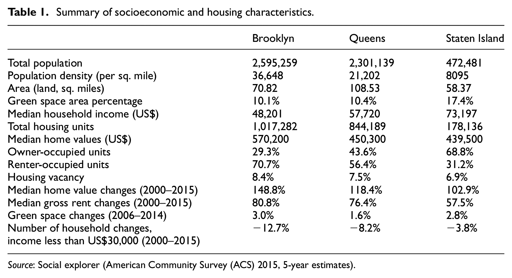
Source: Social explorer (American Community Survey (ACS) 2015, 5-year estimates).
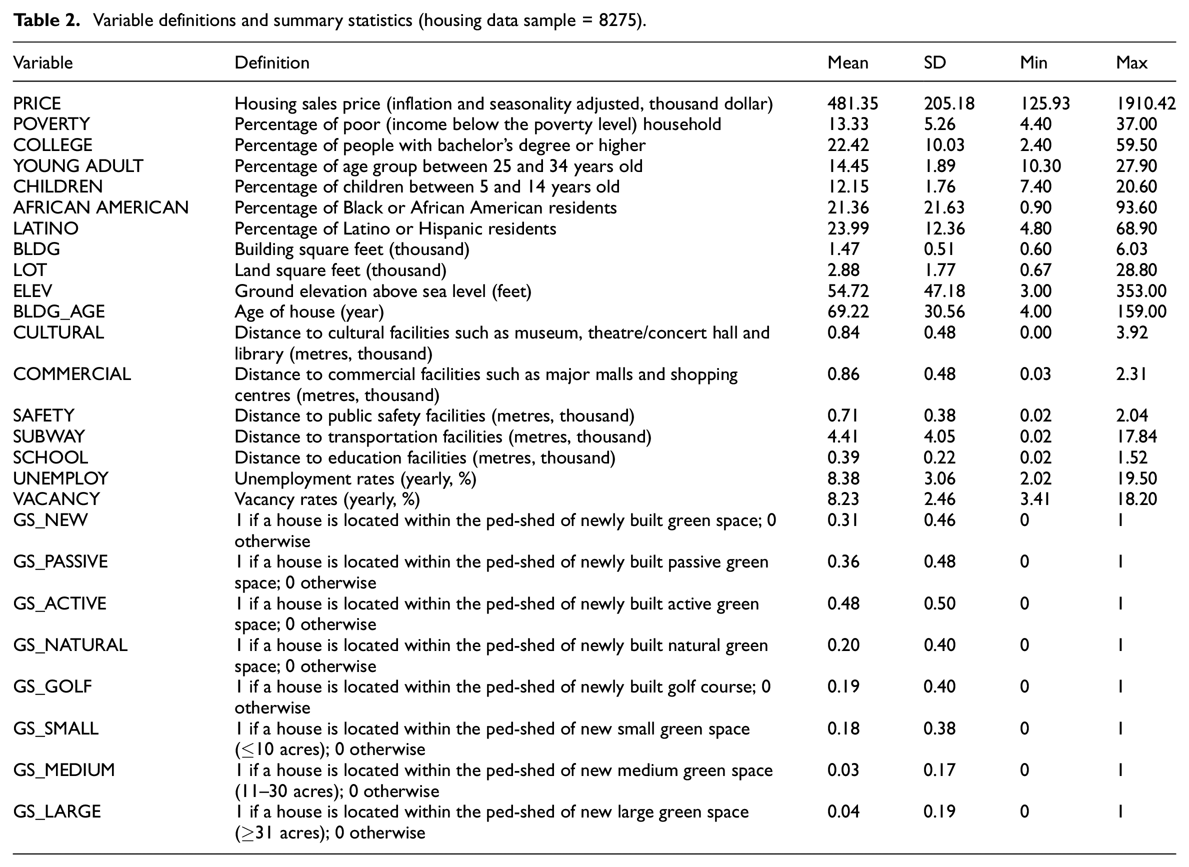
Excluding outliers, such as home prices of less than US$100,000 and more than US$2 million, and multiple duplicate data, a total of 8275 housing sales data were considered to estimate the regression analyses. Lot size, building size, property age and ground elevation variables were used as basic housing structural variables. Public Use Microdata Areas (PUMA) and Census tract-level of unemployment and housing vacancy rates were included to control market idiosyncrasy. To capture locational characteristics, we also included the distance to the neighbourhood’s infrastructural facilities, including cultural facilities (museums, theatres/concert halls, libraries, etc.), commercial facilities (major malls and shopping centres), and public safety, transportation and education facilities.
The necessary GIS data for green spaces, road networks and neighbourhood facilities were obtained from New York City’s open data portal. For all PUMA and census tract-level demographics (unemployment and vacancy rates, poverty rates, educational attainment, young adults aged between 25 and 34, children aged between 5 and 14, and ethnic populations), we used the American Community Survey (ACS) 1-year estimates in each year and non-overlapping 5-year estimates (i.e. 2013 and 2018), respectively, enabling us to estimate the actual change in a relatively shorter period. Although gentrification is generally measured over the longer term, identifying a pattern of those changes within a shorter period contributes to helping guide policymakers, urban planners and other stakeholders to develop more socially inclusive communities.
The green space data, captured from an aerial survey, came from New York City’s planimetric database provided by the Department of Information Technology & Telecommunications. In the same way Holt et al. (2019) and Davern et al. (2017) specified urban green space types by functions and characteristics, the original green spaces were re-categorised according to four distinct types (passive, active and natural green spaces, and golf courses). Each type of green space provides different benefits of health, wellbeing, recreational opportunities, biodiversity and ecosystem services. For example, active green space involves elements that promote physical activities (i.e. running, exercises and biking), while passive green space provides meditation, relaxing spaces. Golf courses and natural green spaces provide different recreational opportunities and ecosystem functions from the other types of green space (Davern et al., 2017). We further classified three reasonably perceivable green space sizes (smaller than 10 acres, 11–30 acres, larger than 30 acres) based on the mean size of the city’s green space (Kim and Peiser, 2018). To separate the effects of green space from those of private backyards, green spaces larger than 0.25 acres were considered in these analyses.
Methods
To test the new green space effect on gentrification empirically, we employed the DiD approach as our main method. Since the effects of green space on the gentrification indicators are localised based on proximity and distance factors, we also used various geospatial processing techniques, including geocoding, near-distance calculation and proximity analysis. Many planning documents define a 400 m (ped-shed) to 800 m (walkshed) radius as ‘walkable catchments’ (roughly taking 5–10 minutes), especially in suburban areas (Ker and Ginn, 2003). As New York City is a densely urbanised city with more roads and crosswalks than less-dense areas, reducing the pedestrian travel time, we constructed the treatment (the impact area within a 400-m buffer) and control groups (outside of the impact area) based on the ped-shed radius for measuring the causal effects of green spaces. For data validity, we conducted a parallel trend test. Appendix 1 demonstrates that the parallel trends assumption (the treatment and control groups follow parallel trends in the absence of the treatment) was not violated.
Although measuring distance based on street networks may better reflect actual pedestrian walking distance to green spaces (Chen, 2017; Higgs et al., 2012; Sevtsuk, 2010), the logged Euclidean distance had a similar accessibility pattern across the city, especially when examining the spatial distance effect at a pedestrian level. To maintain the consistency of all distance variables, we adopted the Euclidean distance in this study. The model was set as follows:
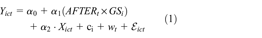
where
Variable definitions and summary statistics (housing data sample = 8275).
Our coefficient of interest
The effects of new green space on gentrification indicators depend significantly on the market responses of movers. If the new green space attracts those who can pay the green space premium, housing price appreciation will be larger for areas near the new green spaces and
Effect of new green space on gentrification indicators (PUMA, 1-year estimates).
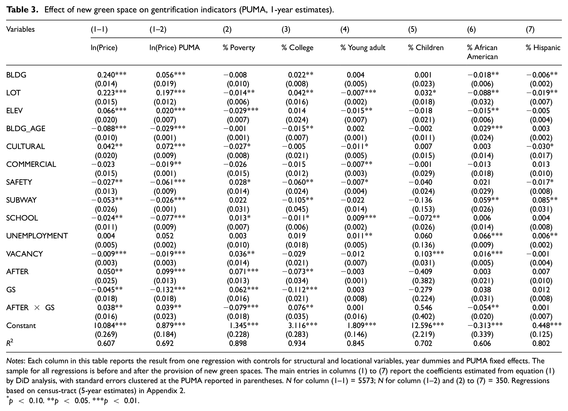
Notes: Each column in this table reports the result from one regression with controls for structural and locational variables, year dummies and PUMA fixed effects. The sample for all regressions is before and after the provision of new green spaces. The main entries in columns (1) to (7) report the coefficients estimated from equation (1) by DiD analysis, with standard errors clustered at the PUMA reported in parentheses. N for column (1–1) = 5573; N for column (1–2) and (2) to (7) = 350. Regressions based on census-tract (5-year estimates) in Appendix 2.
p < 0.10. **p < 0.05. ***p < 0.01.
Effect of green space characteristics on gentrification indicators (PUMA, 1-year estimates).

Notes: Each column in this table reports the result from one regression with controls for structural and locational variables, year and quarter dummies and PUMA fixed effects. The sample for all regressions is before and after the provision of new green spaces. The main entries in columns (1) to (5) report the coefficients estimated from equation (2) by DiD analysis, with standard errors clustered at the PUMA reported in parentheses. Full regressions in Appendix 3. N for column (1) = 5573; N for column (2) to (5) = 350.
p < 0.10. **p < 0.05. ***p < 0.01.
Effect of green space characteristics on gentrification indicators (census-tract, 5-year estimates).

Notes: Each column in this table reports the result from one regression with controls for structural and locational variables, year and quarter dummies and census-tract fixed effects. The sample for all regressions is before and after the provision of new green spaces. The main entries in columns (1) to (5) report the coefficients estimated from equation (2) by DiD analysis, with standard errors clustered at the census-tract reported in parentheses. Full regressions in Appendix 4. N for column (1) = 2024; N for column (2) to (5) = 154.
p < 0.10. **p < 0.05. ***p < 0.01.
To find the causal effects of green space characteristics on gentrification, we employed the following regression equation for testing these criteria:
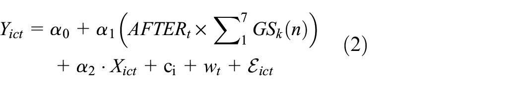
We used the green space characteristics in this setting, where
Results and discussion
New green space effects on gentrification
Our estimates to determine the effect of new green space on gentrification are summarised in Table 3. Each of the columns reports the regression results from one estimate using the DiD method shown in equation (1). We found that new green space affects gentrification by increasing housing prices (column 1–1 and 1–2) and the percentage of college degree attainment (column 3) while decreasing the poverty rate (column 2) and the percentage of African American residents (column 6). The results in columns 4, 5 and 7 indicate that new green space is not statistically meaningful to age groups (25–34 and 5–14 years old) and the percentage of Hispanic residents as indicators of gentrification at any conventional levels of statistical significance. The results between columns 1–1 and 1–2 (Table 3) are broadly the same, and thus we confirm that our DiD estimates do not suffer from the modifiable areal unit problem.
The effects of green space characteristics on gentrification
With respect to the gentrification effects by green space characteristics described in equation (2), the results in Tables 4 and 5 indicate that natural and passive, and medium-sized green spaces strongly affect all four identified gentrification indicators from section ‘New green space effects on gentrification’ (full regressions are presented in Appendices 3 and 4). The coefficients of active green space, golf course and small-sized green space are not statically significant at the 5% significance level. The effects of large-sized green spaces are inconsistent among the selected gentrification indicators –Tables 4 and 5 exhibit a positive impact in housing prices and negative impact in percentage of African American residents, while the coefficients in percentages of poverty and college do not meet any conventional statistical significance criteria. The results support our hypothesis that the new green space effects on gentrification could be different according to each characteristic of green space over a relatively short period.
It is interesting to note that the coefficient of active green space is in contrast to the empirical findings of existing literature (Rigolon and Németh, 2020). One reason is that this model primarily measures the walkable accessibility, rather than close proximity. Thus, the proximity-sensitive health benefits (having more opportunity to engage in physical exercise, especially in the dense urban setting) of active green space such as playgrounds and ballparks may be underestimated. Another postulation is that possible ‘disamenity’ effects (noise, crowdedness, traffic congestion, etc.) caused by active green spaces could decrease demand by home buyers. Although the disamenity effect remains strong directly adjacent to the green space and diminishes over distance, these negative externalities associated with such disamenity could affect housing prices up to 400 m distance or even farther (Chen and Jim, 2010; Netusil, 2005). A possible reason that golf course is positively associated with education attainment at the 10% significance level could be its view and proximity for users. While golf courses impact adjacent housing prices through the attractive views they afford, properties without a golf course view in the vicinity still receive benefits from their location when they use the golf course (Do and Grudnitski, 1995). Higher education may increase the opportunity to use golf courses because residents who have a higher education attainment could earn more salary (Bureau of the Census, 1994). Furthermore, since the effects of green space are spatially proportional to the green space size (Crompton and Nicholls, 2020), the small-sized green space may impact only a few homes immediately nearby: the greater numbers of housing within the ped-shed area remain unimpacted. In addition, unlike large green space projects which often link recreation, tourism and real estate development, small green space generally does not stimulate private development (Rigolon and Németh, 2018). Although adjacent housing prices can be positively influenced by small-sized green space (Tables 4 and 5) that may improve the environment quality nearby, its development scale may be insufficient to attract private investments (including the influx of affluent residents) and consequently could not catalyse environmental gentrification.
Different from previous studies, this study focuses on estimating short-term gentrification effects of green space based on detailed data collected over a different period (i.e. 1-year estimates versus 5-year estimates) with different spatial scales (i.e. PUMA versus census-tract level). Our results support the primary notion that green gentrification can be catalysed or mitigated depending on green space characteristics nearby over relatively shorter periods. The results signify that passive, natural and medium-sized green spaces can contribute to leading gentrification, while active and small-sized green spaces nearby tend to alleviate gentrification to some extent.
Conclusion
Public green space has been viewed as a positive component in urban development because it provides recreational opportunities, health benefits and ecosystem services. However, from a socio-economic perspective as a whole neighbourhood, green space can induce negative externalities, such as gentrification. A number of recent studies have examined the relationship between environmental amenities and gentrification. This study, which also empirically analyses the local effects of public green space on gentrification, is novel in three respects. First, we examine the effect of multiple green space types and characteristics on gentrification indicators jointly. Second, we use a different specification, the DiD framework, to identify the causal inference between attributes of new green space and gentrification. Finally, our study estimates a relatively short- and mid-term gentrification effect in a homogeneous institutional and geographical setting based on detailed census data collected over different periods at different spatial scales.
Since all types of green space have different environmental/amenity functions, their impacts on housing prices and other fundamental factors of gentrification can vary (Czembrowski and Kronenberg, 2016; Panduro and Veie, 2013). Our empirical analysis suggests that certain green spaces, depending on type and characteristics, do in fact affect gentrification indicators. The results indicate that passive, natural and medium-sized green spaces potentially catalyse gentrification over a relatively shorter period by increasing housing prices and the percentage of college degree attainment while decreasing the poverty rate and percentage of African American residents.
Our findings support Wolch et al. (2014)’s claim that small parks do not catalyse green gentrification, which is in contrast to Rigolon and Németh (2020)’s finding that different sizes of new parks do not affect gentrification. The strong gentrification effect of passive and natural green space is consistent with existing green space literature, which suggests that closer proximity to passive or natural open space yields housing price premiums. Our study on census tract levels in a homogeneous urban setting suggests a more careful spatial disposition and mixed-use of green space, particularly with the characteristics that are associated with active and small-sized green spaces to help alleviate gentrification. It must be noted, however, that this study is limited by its focus on a quantitative approach. Not only the number of green spaces but also the subjective quality of green space can impact gentrification. Thus, those qualitative factors require more attention in future studies.
Given that environmental gentrification has become problematic for social justice, it is vital to consider the potentially deleterious side effects during urban revitalisation processes and other public/private investments. Although focusing on single-family home sales in this study could be another limitation of our study, our results broadly support enabling planners and policy stakeholders to create more inclusive and more equitable outcomes by optimising the use of green space characteristics.
Footnotes
Appendix
Full set of DiD estimations (combined model with green space sizes; census-tract, 5-year estimates).

| Variables | ln(Price) | % Poverty | % College | % African American |
|---|---|---|---|---|
| BLDG | 0.218*** (0.023) | −0.097*** (0.030) | 0.061*** (0.015) | −0.015** (0.010) |
| LOT | 0.197*** (0.022) | −0.199*** (0.052) | 0.033* (0.019) | −0.065** (0.032) |
| ELEV | 0.060** (0.028) | 0.014 (0.016) | 0.020 (0.024) | 0.017*** (0.006) |
| BLDG_AGE | −0.074*** (0.014) | 0.070*** (0.023) | −0.006 (0.011) | 0.034** (0.019) |
| CULTURAL | 0.054** (0.024) | −0.019 (0.020) | −0.008 (0.028) | 0.009 (0.023) |
| COMMERCIAL | −0.017 (0.022) | −0.036 (0.025) | −0.026* (0.014) | −0.016 (0.021) |
| SAFETY | −0.030 (0.022) | 0.001 (0.013) | −0.080*** (0.029) | 0.021 (0.022) |
| SUBWAY | −0.019 (0.030) | 0.013 (0.013) | −0.106** (0.051) | 0.059*** (0.017) |
| SCHOOL | −0.022 (0.014) | −0.008 (0.006) | −0.015** (0.006) | 0.001 (0.022) |
| UNEMPLOYMENT | 0.005 (0.005) | 0.045* (0.023) | 0.046 (0.025) | 0.067*** (0.006) |
| VACANCY | −0.006 (0.004) | 0.031** (0.021) | −0.021 (0.013) | 0.022*** (0.006) |
| AFTER | 0.050** (0.025) | 0.071** (0.029) | −0.073** (0.028) | 0.003 (0.022) |
| GS (passive) | −0.207*** (0.033) | 0.025 (0.026) | −0.069 (0.046) | 0.032* (0.019) |
| AFTER × GS (passive) | 0.042** (0.020) | −0.063** (0.037) | 0.046** (0.044) | −0.030** (0.026) |
| GS (active) | 0.022 (0.025) | −0.008 (0.038) | 0.055 (0.040) | −0.004 (0.040) |
| AFTER × GS (active) | 0.004 (0.018) | 0.026 (0.055) | −0.069 (0.050) | 0.004 (0.041) |
| GS (natural) | −0.060* (0.034) | 0.067 (0.048) | −0.021 (0.046) | 0.045** (0.018) |
| AFTER × GS (natural) | 0.066** (0.027) | −0.221*** (0.072) | 0.099** (0.054) | −0.056** (0.023) |
| GS (golf) | 0.067*** (0.018) | −0.024 (0.016) | −0.025* (0.014) | 0.043*** (0.015) |
| AFTER × GS (golf) | 0.002 (0.029) | 0.013 (0.026) | 0.055* (0.021) | −0.021 (0.017) |
| GS (small) | −0.071*** (0.025) | 0.062** (0.029) | −0.016 (0.032) | −0.042 (0.049) |
| AFTER × GS (small) | 0.073* (0.024) | −0.146 (0.053) | 0.141 (0.054) | 0.065 (0.040) |
| GS (medium) | 0.004 (0.073) | 0.062 (0.114) | −0.132 (0.098) | 0.071 (0.058) |
| AFTER × GS (medium) | 0.058** (0.080) | −0.089** (0.187) | 0.289** (0.198) | −0.248*** (0.047) |
| GS (large) | −0.181*** (0.066) | 0.023 (0.053) | 0.036 (0.054) | −0.022 (0.033) |
| AFTER × GS (large) | 0.050** (0.040) | −0.018 (0.069) | 0.014 (0.051) | −0.073** (0.033) |
| Constant | 10.250*** (0.416) | 3.042*** (0.594) | 2.693*** (0.378) | −0.672** (0.377) |
| R 2 | 0.628 | 0.892 | 0.928 | 0.623 |
Notes: Each column in this table reports the result from one regression with controls for structural and locational variables, year dummies and census-tract fixed effects. The sample for all regressions is before and after the provision of new green spaces. The main entries in columns (1) to (4) report the coefficients estimated from equation (2) by DiD analysis, with standard errors clustered at the census-tract reported in parentheses. N for column (1) = 2024; N for column (2) to (7) = 154.
p < 0.10. **p < 0.05. ***p < 0.01.
Declaration of conflicting interests
The author(s) declared no potential conflicts of interest with respect to the research, authorship, and/or publication of this article.
Funding
The author(s) received no financial support for the research, authorship, and/or publication of this article.