



Abstract
This study uses meta-analysis to examine the relationship between estimated international tourism demand elasticities and the data characteristics and study features that may affect such empirical estimates. By reviewing 195 studies published during the period 1961–2011, the meta-regression analysis shows that origin, destination, time period, modeling method, data frequency, the inclusion/omission of other explanatory variables and their measures, and sample size all significantly influence the estimates of the demand elasticities generated by a model. Moreover, the demand elasticities at both product and destination levels are generalized by statistically integrating previous empirical estimates. The findings of this meta-analysis will be useful wherever an understanding of the drivers of tourism demand is critically important.
Introduction
The last five decades have seen a rapid increase in worldwide tourism demand. As a result, international tourism has become increasingly important for worldwide economic development. Both the public and private sectors have channeled substantial resources into the industry. Furthermore, as both governments and businesses need high-quality tourism demand analysis to develop efficient public policy and make good business decisions, considerable efforts have been made to analyze tourism demand and develop explanatory models which help to inform these critical decisions.
Several variables have been suggested as the leading determinants of international tourism demand. However, the estimated demand elasticity of each determinant has been found in previous research to vary significantly across studies which have estimated elasticities empirically. How much of this variation is due to different data measurements, estimation methods, origins and destinations, and other study features and characteristics, and how much of the variation arises from inherent cultural and situational factors is unclear. Some researchers have tried to investigate the general effects of income and price on international tourism demand based on demand theory. These studies have partially succeeded in synthesizing the demand elasticities of aggregate demand, but have failed to analyze disaggregated demand. Past meta-analyses (Crouch 1992, 1995, 1996; Lim 1997, 1999; Brons et al. 2002) of tourism demand focus mainly on evaluating the single effect of either data characteristics or study features on estimates of tourism demand elasticities. No study so far has tried to explore the interactive effects of the two factors combined. Further, in the past 10 to 20 years a considerable number of additional demand studies have accumulated producing a much larger set of estimated demand elasticities. This current study sets out to fill these gaps and to cover the full set of results available to date.
Through a comprehensive review and integration of 195 articles on tourism demand modeling over the period 1961–2011, this study sets out to identify whether there is any association between the estimated international tourism demand elasticities and data characteristics/study features, and how much of this explanatory noise can be eliminated in order to remove some of the “fog” that obscures the generalizability of the results. An attempt will be made to compare the magnitudes of the impacts of the influencing factors on tourism demand across studies. Through generalizing the demand elasticities at a disaggregated level, it will help to enhance our understanding of tourist behavior and the diversification of tourists’ tastes, and also help in the development of more effective international tourism forecasts, and development and investment strategies including public policy, marketing programs, and efforts to maintain and enhance destination competitiveness.
Literature Review
The identification, analysis, and measurement of the impacts of the determinants of tourism demand are central to any effort to understand and explain changes in demand in the past and to anticipate the possible pathways of future tourism demand development. A number of variables have generally been examined and accepted in previous research as the main determinants of international tourism demand. However, significant distinctions can be drawn between the influences of different determinants for different visit purposes. For example, Turner and Witt (2001) show that the volume of international trade is closely associated with business tourism demand, but that the volume of retail sales is more closely associated with the demand for holiday tourism, and the demand for visits to friends and relatives (VFR) is linked more to overall gross domestic product (GDP).
Income in source markets has been demonstrated in past research to be a dominant explanatory variable and is the most widely discussed determinant of international tourism demand. Most researchers employ either nominal or real GDP or gross national product (GNP), or their per capita forms, as a suitable measure of tourists’ income (see, e.g., Greenidge 2001; Turner and Witt 2001). Other less commonly used measures of income include real consumption per capita (Dritsakis 2004); superfluous income that is defined as real disposable income less expenditure on food, housing, fuel, and power (Edwards 1979); foreign travel budgets (Smeral and Witt 1996); industrial production indices (Gonzalez and Moral 1995); and real household disposable income (Lim 1997).
Most of the empirical studies demonstrate that in accordance with economic theory, income has a positive effect on tourism demand. They also conclude that international tourism is a luxury product as indicated by the fact that most studies have estimated an income elasticity of demand exceeding the value of 1.0, which shows that, as income rises, tourism consumers spend an increasing proportion of their income on international travel. According to a meta-analysis of 1,501 estimates by Crouch (1996), the mean income elasticity was found to be 1.86, with a standard deviation of 1.78. Crouch (1992) also suggested that different estimates arise depending on the different income measures employed (e.g., total income vs. per capita income). When holiday visits or VFR travel are under consideration, the more appropriate form of the income variable is private consumption or personal disposable income, while a general income measure is more appropriate for business visits. Moreover, income elasticity may differ considerably across different origin–destination pairs. For example, the estimated income elasticity of the demand for Aruba tourism varies from 1.43 for U.S. tourists to 2.52 for Dutch visitors (Croes and Vanegas 2005). By contrast, Naude and Saayman (2005) show that the level of income in origin countries has little effect on the demand for tourism in Africa.
The relative price of tourism is another important determinant of demand. Estimated price elasticities are nearly always negative demonstrating that rising prices deter demand. The consumer price index (CPI) of the destination country divided by the CPI of the origin country is the most frequently used proxy variable to capture relative price effects. Some studies opt to use specific tourism price variables, such as service price indexes (Cheung and Law 2001), hotel price indexes (Narayan 2004), or the weighted prices of food, accommodation, transport, entertainment, and other services (Dwyer, Forsyth, and Rao 2000). Exchange rates are also often used to adjust relative prices or may be included in the demand model as a separate variable on the basis that tourists may display different sensitivities to actual price changes versus variations in exchange rates (Webber 2001; Croes and Vanegas 2005; Mangion, Durbarry, and Sinclair 2005). Tourists tend to be more aware of exchange rate changes before they travel than they are of inflationary effects in the destination they plan to visit.
Transportation costs can account for a large proportion of tourism expenditure, and are often measured by the cost of air travel (Turner and Witt 2001), travel distance, and gasoline costs (Martin and Witt 1988). However, studies using travel exports/imports as a dependent variable do not fully support the idea that international tourism demand is inversely related to transport costs (Lim 1999). According to Crouch’s (1996) meta-analysis, the price elasticity of tourism demand has a mean value of −0.63, with a standard deviation of 2.32. He attributes this variation principally to sampling errors. Furthermore, price elasticities vary considerably among different origin–destination country pairs (Mangion, Durbarry, and Sinclair 2005) and by trip purpose (Sakai 1988; Lehto, Morrison, and O’Leary 2001). Data frequency, the number of explanatory variables in the models, and their definitions are also believed to influence the various elasticity estimates (Crouch 1992, 1996).
Other potentially significant determinants that have been discussed in previous studies include prices in substitute or alternative destinations, which could be measured by domestic CPI or a weighted tourism price for a set of substitute destinations (Witt and Witt 1995; Song and Wong 2003); the size of the population within the origin (Witt and Martin 1987; Turner and Witt 2001); trends in immigration patterns (Seetaram and Dwyer 2009); destination promotional expenditure, which, if effective, ought to stimulate tourism demand (Crouch, Schultz, and Valerio 1992); changes in tourists’ tastes, which could be captured by time trends; seasonal variations (Lim 2004); climate change (Lise and Tol 2002); political instability (Dhariwal 2005; Naude and Saayman 2005); foreign direct investment, which relates mainly to business travel (Tang, Selvanathan, and Selvanathan 2007); the educational level of tourists and their age distribution (Alegre and Pou 2004); rates of unemployment (Cho 2001); the levels of income distribution and inequality (Morley 1998); one-off events such as acts of terrorism or infectious disease scares (Song and Lin 2010; Smeral 2010); and the lagged effects of both explanatory variables as well as the dependent variable itself, which can be an indicator of the strength or durability of habit persistence in travel preferences.
Hypotheses
Previous work supports the idea that the estimates of demand elasticities are related to the characteristics of the data used and also to the key features of each study, such as data frequency, alternative measures of demand, the particular origins and destinations under study, and travel distance (Crouch 1992, 1996; Song, Witt, and Li 2009). In this section, a series of hypotheses will be developed to explore the effects of data and study characteristics on estimates of income and own-price elasticity.
Under the influence of different economic conditions and cultural and customer habits, the income and price sensitivities of tourists from different origins would be expected to vary. Crouch (1996) used dummy variables to test the effects of different origins and destinations on the estimated demand elasticity of international tourism and found that the country dummies were statistically significant. He found that tourists from developed regions tend to view international tourism as less of a luxury than those from less developed countries. Tourists from countries where international travel is common are likely to be less sensitive to income and price changes. Living in countries with large geographic areas, tourists tend to have more options for holidaying within their national boundaries and may therefore be more sensitive to changes in the price of international tourism, everything else being equal (Little 1980). Therefore, we hypothesize that the estimated income and price elasticities of international tourism demand vary by source market (hypotheses 1a and 1b).
The characteristics of a destination may influence its uniqueness and popularity and, as a consequence, the income and own-price elasticities of tourism demand. Based on demand theory, income elasticity ought to be lower for destinations regarded as less of a luxury. Anastasopoulos (1984) pointed out that the absolute value of the price elasticity is lower for more unique destinations. For destinations with many substitutes and competitors, price competition tends to be intense and there is likely to be greater sensitivity to price indicative of the greater opportunity to switch between alternative destinations. Therefore, we hypothesize that the estimated income and price elasticities of international tourism demand vary by the destination concerned (hypotheses 2a and 2b).
Analyses conducted to estimate demand elasticities over different time periods are likely to result in different estimates as there is no reason to expect elasticities to be time invariant. During periods of economic prosperity, tourists are more likely to travel and to be less sensitive to income and price changes. During a recession, personal wealth is reduced and income elasticity may increase. Price competition is also very common during economic crises, resulting in higher than normal price elasticity (Song and Lin 2010). Therefore, we hypothesize that the estimated income and price elasticities of international tourism demand vary according to the time period covered by the data (hypotheses 3a and 3b).
The structure and characteristics of different estimation models may influence the estimates of demand elasticities. Traditional regression models assume that income and price elasticities are constant, while the time-varying parameter (TVP) technique permits these parameters to vary over time (Song and Wong 2003). Whether or not the model specification provides for behavioral changes by tourists over time, the estimated demand elasticities would be expected to change. Moreover, in the dynamic models, which include lagged dependent and independent variables, the effects of tourists’ loyalty and “word of mouth” are able to be separately estimated. In these dynamic models, both long-run and short-run elasticities may be estimated. Therefore, we hypothesize that the estimated income and price elasticities of international tourism demand vary according to the modeling methods used for the estimation (hypotheses 4a and 4b).
The use of different data frequencies in demand studies is evidence that researchers have different concerns in terms of the time-dependent response to changes in the explanatory variables, and estimates of demand elasticity may vary depending on data frequency. Crouch (1996) suggests that the estimated income elasticities will increase with increased data frequency, and that price elasticity will also vary as a function of the time interval used. Hence, we hypothesize that the estimated income and price elasticities of international tourism demand vary according to the frequency of data employed (hypotheses 5a and 5b).
Econometric studies show that the omission of relevant variables in a regression model may bias the estimated coefficients of the other explanatory variables (Gujarati 2003, pp. 508–9). The magnitude of such bias will depend on the relationship between the omitted variable, the dependent variable, and the other explanatory variables. Economic variables, such as income, own price, substitute prices, exchange rates, and travel costs, are often collinear. Accordingly, we hypothesize that the omission of explanatory variables will bias the estimates of income and price elasticities of international tourism demand (hypotheses 6a and 6b). For the same reason, we hypothesize that the estimated income and price elasticities of international tourism demand vary according to the absolute number of explanatory variables included in the estimation model (hypotheses 7a and 7b).
Keele and Kelly (2006) show that the inclusion of a lagged dependent variable may affect the estimates of the coefficients of the other explanatory variables in the model. Since the lagged dependent variables in a model are likely to be correlated with the other explanatory variables, the length of the lags may influence the estimates of demand elasticities. Therefore, we hypothesize that the estimated income and price elasticities of international tourism demand vary according to the lag length of the (lagged) dependent variable in the model (hypotheses 8a and 8b).
Since travel costs can account for a major part of tourism expenditure, it is to be anticipated that tourism consumers would regard long-haul tourism as more of a luxury compared to short-haul tourism and that this difference would show up in estimated elasticities of demand. Even with the advent of low-cost carriers, travel costs usually still increase with distance traveled. Therefore, long-haul tourism is usually more expensive and has higher income elasticity than short-haul tourism. However, Anastasopoulos (1984) suggests that as long-haul tourists tend to come from more wealthy regions, they may therefore be less income sensitive, potentially offsetting this effect. Turning to price elasticity, long-haul tourists are less sensitive to price changes than short-haul tourists, according to Crouch (1994b) and Brons et al. (2002). This may be because of the more exotic, unique features of such destinations and therefore the lack of available substitutes. Therefore, we hypothesize that the estimated income and price elasticities of international tourism demand vary according to travel distance (hypotheses 9a and 9b).
Tourism demand has been measured in a variety of ways in previous research, with some studies even using more than one dependent variable to represent demand. By reviewing studies published between 1961 and 2004, Crouch (1994a), Lim (1997), and Li, Song and Witt (2005) summarize four demand measures that are commonly used. These include the number of tourist arrivals, the quantity of tourist expenditure/receipts, length of stay, and the number of nights spent at tourist accommodation. Of these measures, tourist arrivals and expenditure and their derivatives (such as arrivals and receipts divided by population of the origin) are the most frequently used in the demand modeling literature. The different measures of tourism demand may be expected to influence the estimates of demand elasticities. With the progressive development and promotion of international tourism, and the overall decline in the real cost of such travel, more and more people now travel internationally. Travel attitudes and habits have therefore changed and evolved over time. As a result, tourism has become a much more common experience for a growing number of people who regard international travel as an experience they are now more habituated to. Instead of reducing the number of trips taken, tourists may tend to reduce their expenditure per trip or length of stay in response to declining economic or other adverse conditions. Therefore, we hypothesize that the estimated income and (absolute values of the) price elasticities of international tourism demand are higher when demand is measured by expenditure/receipts than by other means (hypotheses 10a and 10b).
As well as using total tourism demand data, some researchers have employed disaggregated data to examine tourist demand at the product level, including accommodation, dining, and shopping. Law and Au (2000) conclude that income and price elasticities vary significantly across classes of tourism products. It is therefore expected that the estimated income and price elasticities of international tourism demand may vary according to the level of aggregation in international tourism demand measurement (hypotheses 11a and 11b).
Income in the origin, as the most commonly used determinant of international tourism demand, can be expressed in either aggregate or per capita form. As population and income both tend to increase over time, aggregate income rises faster than per capita income. Hence demand should be more responsive to per capita changes. Therefore, we hypothesize that the estimated income elasticities of international tourism demand are higher when the income variable is measured in per capita form (hypothesis 12a ).
The year in which the research is published may be analyzed as a proxy measure of any time trend in tourism demand sensitivity. With the growth in consumer incomes and the declining real cost of air travel, international tourism has become more common worldwide and therefore less of a luxury, so income elasticities may have declined over time as a result. With the development of the tourism industry, more destinations are emerging and tourists have more channels than before through which to access information about them. As tourists have more choices and have become more aware of tourism costs, the absolute values of the estimated price elasticities in more recent studies are likely to be higher than was found in studies published in the past covering older data. Therefore, we hypothesize that the estimated income elasticities of international tourism demand have a negative relationship with the year of publication of the study (hypothesis 13a) and the (absolute values of the) estimated own-price elasticities of international tourism demand have a positive relationship with the year of publication of the study (hypothesis 13b).
The data sample size has been shown to be correlated with the estimates of coefficients (Glass, McGaw, and Lee 1981). Crouch (1992) shows that estimated demand elasticities vary significantly across different sample sizes. Therefore, we also hypothesize that the estimated income and price elasticities of international tourism demand vary according to the sample size (hypotheses 14a and 14b).
Tourists usually plan international travel several weeks or months ahead. In the short term, their response to income and price changes may be constrained by existing travel arrangements. However, in the long run, they have enough time to fully adjust their behavior and are likely to display more income- and price-elastic behavior. Therefore, we hypothesize that the estimated long-run income and (absolute) price elasticities of international tourism demand are higher than the short-term estimates (hypotheses 15a and 15b).
Methodology
Meta-analysis techniques are applied to examine the impact of data characteristics and study features on the demand elasticities for international tourism. Meta-analysis has the power to generate a true effect size through a comprehensive and systematic review of the findings from past studies, which improves the validity of the conclusions and is helpful in explaining variations across studies. The application of meta-analysis in tourism demand analysis has so far been very limited. The only studies are those by Crouch (1992, 1995, 1996), Lim (1997, 1999), and Brons et al. (2002). However, in many other fields, meta-analysis is a widely used technique for synthesizing results across a large number of empirical studies in order to identify the degree of consensus and disagreement in their findings, and thereby to generalize overall conclusions.
The first step of any meta-analysis is to locate as many relevant empirical studies as possible. Google Scholar was first used to find articles containing at least one of the expressions “tourism demand” or “tourism modeling” over the time period 1961–2011. This time period was selected for two reasons. First, 1961 was the year in which the earliest known work that included international tourism demand elasticity estimates was published (Guthrie 1961). Second, the aim was to extend the sample size to include most if not all of the published studies that reported international tourism demand elasticity estimates, so that a more comprehensive and up-to-date meta-analysis could be carried out compared to previous studies. Google Scholar was selected as the search engine mainly for its comprehensive coverage of English-language articles in various disciplines and its reputation among academics. Following the primary website search, referencing and footnote chasing was used to ensure the comprehensiveness of the articles identified. After identifying potential sources, some studies were rejected according to the following exclusion criteria: (1) the article did not report empirical estimates of income or own-price elasticities, (2) the article was not written in English, or (3) the article reported demand elasticities that had already been included in the data set (to avoid double counting of the estimated demand elasticities). The final set of articles included in this study is summarized in Table 1, together with the number of estimated demand elasticities available from each.
Articles Reporting Demand Elasticities of International Tourism.

For the purpose of our meta-analysis, we used a regression technique (meta-regression hereafter) in order to identify and evaluate simultaneously the effects of the independent variables on the dependent variables. The estimated own-price and income elasticities become the dependent variables, whereas the various data characteristics and study features outlined above represent the independent or explanatory variables. Following the process suggested by Sargan (1964), if

where Y refers to the reported income or own-price elasticity of international tourism demand; X is a matrix of explanatory variables; β is the parameter matrix to be estimated, indicating the fractional change of Y in response to a one-unit change in X; C is the intercept vector; and µ refers to the residual vector. The explanatory variables include continuous variables, such as year of publication, number of variables included in the study, lag length of the dependent variables and sample size; and a set of dummy variables. To avoid the invalidity of statistical tests caused by heteroskedasticity, the weighted least squares method is applied in the parameter estimation, assuming that the error term is normally distributed.
Dummy variables were used to analyze the effect of the various categorical and ordinal variables. The dummy variables that capture the effects of the source markets and destination regions are defined for both origins and destinations as a series of five 0–1 dummies, using a sixth other destination/origin category as the dummy comparison benchmark, where each takes the value of 1 if the estimated elasticity is associated with the origin/destination concerned, or 0 otherwise. The five dummies are associated with Europe, America, Oceania, Asia, or Africa. The benchmark category covered those studies that did not specify the origin and destinations. Hence, 5 dummy variables capture the influence of the origin and likewise 5 also capture destination effects. With regard to the year of study, there were four separate dummies each taking the value of 1 if the study was conducted respectively in either the 1970s, 1980s, 1990s, or 2000s and 0 if not. By omitting a dummy for estimates from other than one of these four periods, the regression coefficient therefore uses the period before 1970 as the comparison benchmark. Two dummy variables were used to model the data frequency. Each of these took the value of 1 respectively if either monthly or quarterly data were used and 0 otherwise. As no dummy was used for annual data, the regression coefficients for the two dummies can therefore be interpreted in comparison with the annual benchmark. Similarly, two dummies were used to model the three modeling methodology categories with “static econometrics” as the benchmark category; the dummies take the value of 1 if the study used either the advanced time series, or alternatively the dynamic econometric models, and 0 if the other two models were used. The omission of explanatory variables from the estimation models was analyzed using five further dummy variables for each of income, own-price, substitute-price, exchange rate, and travel cost. The benchmark for these dummies was the case where all five of these variables were included. One dummy was used to model the effect of travel distance by representing the effect of intercontinental tourism demand analysis compared to intracontinental (or not specified) travel. Three further dummies, each with their own benchmark, were used to assess the effect that the method of defining and measuring the demand variable had on the resulting elasticity estimates. These three dummies considered whether or not demand was measured in the form of tourist expenditure (where not this was commonly tourist numbers), whether the demand measured a particular product type or was instead aggregate demand to the destination, and whether or not the demand was in per capita form. Finally, one dummy was used to model the adjustment period (set to 1 for short-run estimates against a benchmark of long-run estimates).
The meta-regression estimations follow the general-to-specific process (see the detailed explanation in Song and Witt 2003), in which variables that are insignificant at the 5% level or contradict economic theory are removed until all the remaining coefficients in the models are significantly different from zero and consistent with theoretical restrictions.
A further task is to generalize the elasticities at the product or origin/destination level. As few studies reported the variance of the estimates, only a simple average for the elasticities is summarized. The mean elasticities for different data groups are also summarized.
Data Description
A comprehensive search of the literature generated 702 articles on international tourism demand analysis. Based on the selection criteria, 195 studies were selected for the meta-analysis comprising a total of 2,833 estimated demand elasticities (1,633 income elasticities and 1,203 own-price elasticities). Since the single log-linear meta-regression model is to be preferred in this analysis, as noted above, the application of this specification to the data requires only positive values of Y. In the case of the estimated own-price elasticities, which are expected to be negative, and indeed were for all but 8% of the estimates, nonnegative estimates were excluded from the analysis in order to facilitate the meta-regression as well as to accord with theoretical expectations. The sources and distribution of these estimates are summarized in Table 1.
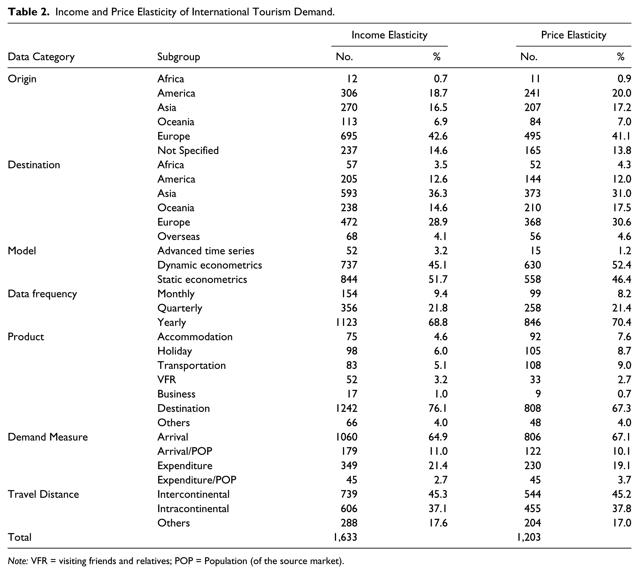
Table 2 profiles each data set. European countries are the most frequently studied source markets for international tourism. In total, 695 estimates (42.6%) of income and 495 (41.1%) of price elasticities were related to European tourists. Only seven studies (12 estimates) analyzed the income elasticities of African tourists, with five studies (11 estimates) reporting price elasticities.
Income and Price Elasticity of International Tourism Demand.
Note: VFR = visiting friends and relatives; POP = Population (of the source market)
The most studied destination regions were Asia and Europe. Income elasticity estimates of tourists traveling to Asia and Europe account for 593 (36.3%) and 472 (28.9%) values, respectively. Own-price elasticity estimates for Asian and European destinations account for 373 (31.0%) and 368 (30.6%) values, respectively. In terms of travel distance, intercontinental tourism commonly defines long-haul tourism and intracontinental tourism is normally regarded as short-haul tourism. There were more studies in the former category.
Econometric modeling methods have dominated tourism demand analysis. Advanced time-series models were used in only eight studies (52 estimates) to estimate income elasticities of international tourism demand and in only six studies (15 estimates) to estimate own-price elasticities. Dynamic and static econometric models featured in the studies approximately equally, with static econometric models dominating the pre-1995 literature. Dynamic econometric models developed quickly after that, with the autoregressive distributed lag model (ADLM) the most commonly used (293 income and 252 price elasticity estimates).
In terms of data frequency, 1,123 (68.8%) and 846 (70.4%) estimates of income and price elasticities, respectively, were generated using annual data. Yearly data was particularly common in studies conducted before the year 2000. Many studies analyzed international tourists’ behavior at the destination level (76.1% for income elasticity and 67.3% for price elasticity). At the product level, accommodation, transportation, holiday tourism, and VFR tourism were the most frequently studied topics. Tourist arrivals and expenditure, and their per capita forms, were the most commonly used measures of tourism demand. Studies analyzing tourist arrivals accounted for 64.9% and 67.1% of all estimates of income and price elasticities, respectively. The second most popular demand measure was tourism expenditure, leading to 349 (21.4%) and 230 (19.1%) estimates of income and price elasticities, respectively.
Meta-Regression
The results of the two meta-regressions are presented in Table 3. In the case of the various dummy variables discussed earlier, the category selected as the comparator is denoted by the term “benchmark.” The adjusted R2 indicates that the regression models were successful in explaining 23.0% of the variation in estimated income elasticities and 14.7% of the variation in the estimated own-price elasticities. In the context of the meta-analysis literature, such R2 values suggest reasonably typical degrees of fit of the data to the meta-regression models.
Meta-Regression for Tourism Demand Elasticity.

The results of the regression analyses show that both the origin and the destination concerned across the study estimates help to explain a significant portion of the variance in both estimated income and own-price elasticities. In particular, the demand for international tourism by European tourists tends to have much higher income elasticities than by those from other source markets (32.1% higher than the world level). This may be a cultural difference in income sensitivity to international travel, or it may possibly reflect differences arising from the type of destination that Europeans tend to prefer. Asian and African countries and Oceania, as tourism destinations, tend to be associated with lower income elasticities. This could be indicative of perceived lack of luxury. Alternatively, as travel to these locations is more likely to be seen to be something tourists from other countries might only do once, changes in income levels may have limited impacts on once-in-a-lifetime desires.
Compared to tourists from other origins, tourists from Asia and America are more sensitive to price changes in tourism products. Meanwhile, as destinations, Asian, American, and European locations are associated with higher price sensitivities. This result may be indicative of differences in the number of substitutes or competitors leading to higher price elasticities (Little 1980).
The estimated coefficients associated with the dummy variables accounting for the time periods of the data coverage all have significant influences on the estimates of income elasticities. The different signs and values of the coefficients show that the demand elasticities have varied considerably over the past 50 years. This may be due to fluctuations in worldwide economic activity and changes in people’s expectations of their income and job situation (Smeral 2012). This finding also indicates that when estimation models are forced to assume constant income elasticities, estimation error is likely to be greater. However, only the dummy variable for the 1980s was found to be significant in the regression model of price elasticity estimates, which indicates that this parameter has changed little over the decades. The price elasticity in the 1980s was found to be significantly higher compared to the other periods. This may be a product of the oil crisis at the end of the 1970s (Martin and Witt 1987; Lim and McAleer 2002; Song, Witt, and Jensen 2003) or the global economic recession in the early 1980s. These results demonstrate that the estimated income and own-price elasticities of international tourism demand have not remained static.
The meta-regressions show that the estimated income elasticities of international tourism demand also depend on the modeling methods used. Compared to other methods, the dynamic econometric models tend to yield higher income elasticities (13.2% higher than the static models), while own-price elasticity seems instead to be constant across different approaches. This suggests that the complexity and temporal structure of the model will influence the elasticity estimates produced in the case of income.
The income elasticity of tourism demand generated using monthly data is higher than that generated from quarterly and annual data. This indicates that the estimated income elasticities depend on data frequency. Again, however, this was not the case for price elasticity, where no significant effect due to data frequency was found.
The regression results suggest that omission of the substitute-price variable in the demand model would have a negative impact, and omission of the exchange rate variable a positive influence, on the estimates of income elasticity. In the case of price elasticity, the omission of the income variable would have a positive influence, and the omission of the substitute-price and travel cost variables a negative impact. These findings support the hypothesis that omission of other potentially important explanatory variables can significantly influence the estimates of income and own-price elasticities.
The number of variables included in the regression model was found to have a negative influence on the estimates of income elasticity, but no significant effect on price elasticity. The regression results also show that the lag length of the dependent variables included in the models is likely to have a positive effect on estimates of the absolute value of the own-price elasticity. That is to say, the greater the lag effect of the dependent variable included in the model, the higher the absolute price elasticity that results. However, the hypotheses that the lag length of the dependent variable in the model would influence estimated income elasticities is not supported by these results.
The regression results demonstrate that the income elasticity for intercontinental tourism is significantly higher than that for intracontinental tourism. Consistent with economic theory, this indicates that long-haul travelers are more income sensitive than short-haul travelers. The results also show that the price elasticity of international tourism demand does not vary significantly with travel distance.
Somewhat unexpectedly, the meta-regression results show that when tourist expenditure/receipts is used as the measure of international demand, a significant negative effect on estimates of income elasticity is likely to arise. However, with regard to price elasticity, the result supports the hypothesis that tourists’ expenditure is more price elastic when measures involving expenditure/receipts are used. According to the regression results, income elasticity is not greatly affected as a function of whether demand for the whole destination or for specific products is considered. However, when considering the disaggregated international tourism demand for specific products, the means of the absolute price elasticities are significantly lower than for the destination as a whole. This may be because tourists have many potential substitutes when they choose a destination but may be loyal to specific products, such as airplane travel and luxury hotels. Another possible reason is that the articles studying disaggregated tourism products focus primarily on accommodation and transportation, which are necessities for most tourists. It was assumed that the estimated income elasticity of international tourism demand will be higher when the income variable is measured in per capita terms, but the results do not support this hypothesis.
The dummy variable for the short-run estimates shows that international tourists are less sensitive to income and price changes, consistent with expectations. Additionally, the income coefficient for the year of publication is negative, implying that in general international tourists’ sensitivity to income has been gradually declining over the past 50 years. This, however, was not found to be the case for price sensitivity. Together, these two findings are quite consistent with a view that growth in international tourism has led to a decrease in its luxury status, but the growing competition between destinations has resulted in an expansion in the number and range of alternative destinations available, producing today more price-sensitive tourists than in the past.
Sample size also has a significant influence on the estimates of income and price elasticities of international tourism demand, but the magnitudes of the coefficients are very small, which suggests that the effects are rather limited.
To establish the reliability of the regression models reported above, several collinearity diagnostic tests were also carried out. The correlation matrices show that none of the bivariate correlation indexes are larger than 0.8, which indicates no strong linear association between any two variables in the model (Mason and Perreault 1991). The variance inflation factor indexes for all the variables in the regressions are not significantly larger than 10, indicating no significant multicollinearity problem in those models (Marquardt 1970).
Conclusion and Discussion
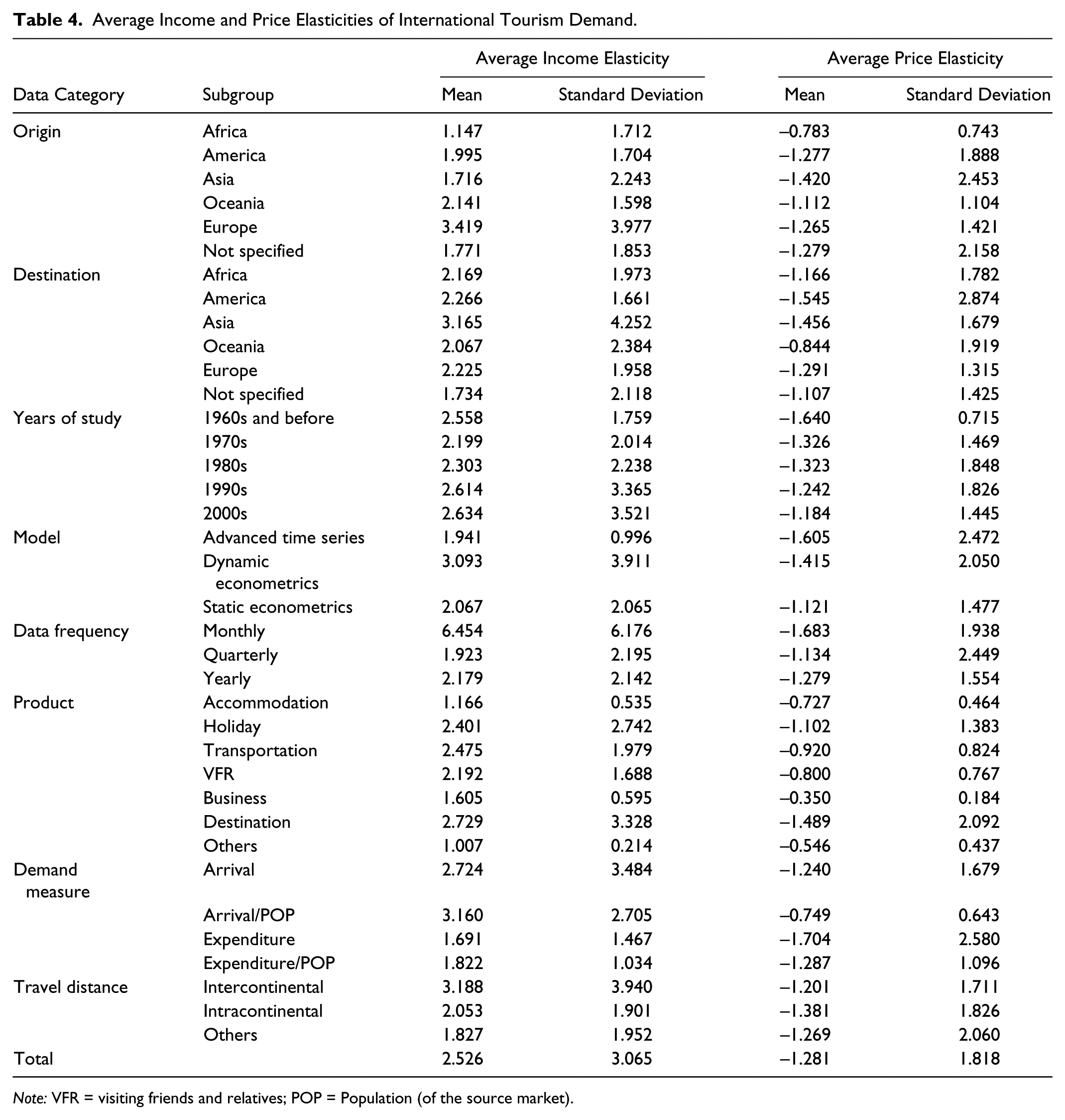
Income and own-price elasticities of international tourism demand reveal tourists’ economic reactions and preferences toward travel in general and toward specific destinations. Such information provides a foundation for destination development planning and the design of marketing strategies. According to the meta-analyses reported and discussed above, the demand elasticities of international tourism vary significantly across different origins, destinations, products, data frequencies, demand variable measures, modeling methods, and in terms of travel distances. Understanding how and why differences in demand elasticities occur is essential if effective destination marketing strategies are to be formulated. To aid in this task, in Table 4 we summarize the average income and own-price elasticities of demand for each explanatory category based on the previous studies.
Average Income and Price Elasticities of International Tourism Demand.
Note: VFR = visiting friends and relatives; POP = Population (of the source market).
The overall average income elasticity of international tourism demand is 2.526. This indicates that, on average, the majority of international travel is clearly in the “luxury” category (economists define luxury products as those with income elasticities greater than 1.0). The overall average price elasticity was found to be −1.281.
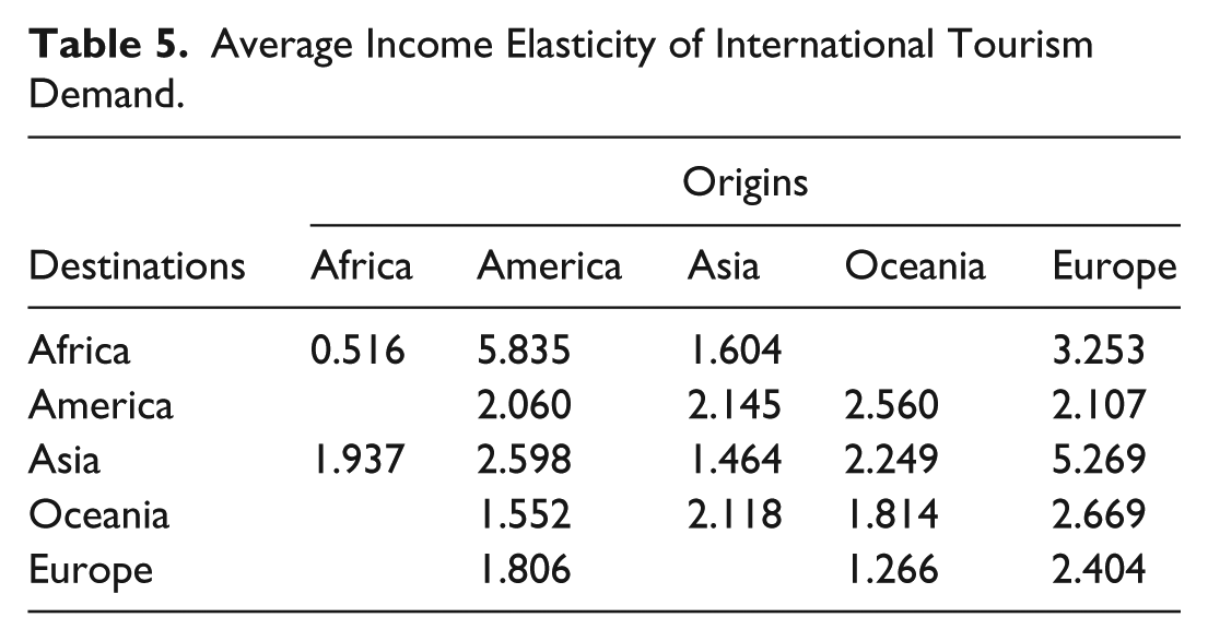
European tourists had the highest income elasticity (3.419), with Africans (mainly South Africans) the lowest (1.147). Tourists who traveled to Asia showed the highest income elasticity (3.165), and the second-highest absolute price (–1.456) elasticity. Tourists to Oceania exhibited the lowest income elasticity (2.067) and were also the least price sensitive, with an average own-price elasticity of −0.844. The average income and price elasticities for each origin–destination pair, where data were available, have also been calculated and are summarized in Tables 5 and 6.
Average Income Elasticity of International Tourism Demand.
Average Price Elasticity of International Tourism Demand.

In terms of modeling methods, the dynamic econometric models produced higher estimates of both income (3.093) and own-price elasticity (–1.415) than were produced by the static models. Studies using monthly data tended to generate higher income (6.454) and absolute price (–1.683) elasticities than those employing lower-frequency data. The income and price elasticities for models using quarterly data were 1.923 and −1.134, respectively.
Different tourism products also have significantly different demand elasticities. Among the products studied, accommodation, which is a necessity for most international tourists, has the lowest income (1.166) and absolute price (–0.727) elasticities. Studies that considered the destination as an aggregated tourism product tended to show the highest income and price elasticities.
The demand for international air travel is the main focus of studies on tourism transportation. Since the substitutes for most travel modes are limited, the average absolute price elasticity of transportation is relatively low (–0.920). Compared to holiday and VFR tourists, business tourism had an average income elasticity of 1.605 and an own-price elasticity of −0.350, which is the lowest of all three tourism products studied. Studies on the demand for medical tourism, although small in number, tend to exhibit much lower income and price elasticities than pleasure tourism. This may be due to the fact that tourists who traveled for medical purposes tended to be richer and their destinations have relatively cheaper but high-quality medical services.
Studies that analyzed tourist arrivals tended to generate greater income (2.724 for all arrivals and 3.160 for arrivals per capita) and lower absolute price (–1.240 for all arrivals and −0.749 for arrivals per capita) elasticities than studies examining expenditure. The findings on the effect of travel distance are consistent with previous studies which concluded that long-haul tourism is considered more of a luxury than short-haul tourism. The income elasticity for intercontinental tourism (3.188) is higher than that for intracontinental tourism.
Overall, the difference between the elasticity estimates for each subgroup indicates that tourists from different source markets, going to different destinations, and consuming different products have different sensitivities to income and price changes. Therefore, different marketing strategies should be applied in different markets. For example, American and Asian tourists were found to be the most sensitive to price changes, so a marketing strategy that emphasizes price may be appropriate. This is less of an issue for Oceania tourists, so in this case it would be better to emphasize the uniqueness of products in marketing activities directed at this group.
Demand elasticities also vary over time, so governments and tourism businesses should design their marketing strategies in response to changing markets and changing travel tastes and preferences. Furthermore, different modeling methods, data frequencies, and demand measures generate different estimates of elasticities, so governments and tourism enterprises should pay particular attention to the data and modeling features of relevant studies when examining the marketing implications.
Compared to the prior meta-analytical studies on international tourism demand, this study has greatly enlarged and updated the coverage of the relevant literature which has now accumulated over the past five decades. However, only published articles were included in the analysis. As scholarly journals are less likely to publish studies that produce results that are of low statistical significance or that run counter to prevailing wisdom, the inclusion of additional unpublished studies, such as working papers, PhD theses, and articles obtained through personal contacts, could be one way to improve the reliability and comprehensiveness of future meta-analytical studies. Moreover, because of the constraints of the sample, only the effects of origins and destinations at the continent level were evaluated in the regressions. With an increase in the volume of published studies in the future, more fine-grained analysis may be possible. For example, the influences of origins and destinations at the country level and specific customer segments could be analyzed in future research. Additionally, interaction effects between particular explanatory variables in the meta-regression may be possible. We have tested the interaction effects between tourism demand measures and other dummy variables; however, unfortunately, limited interactions are significant. With the increasing number of studies in tourism demand modeling, more interaction effects between explanatory variables could be discussed. There may also be some merit in furthering investigation into other explanations behind variations in estimated elasticities. For example, variations in estimates as a function of the time period might more closely examine time trends or the effects of significant international events on tourism. Given the wide range of differing contexts across studies, this may be difficult to investigate at this point in greater detail until further future studies add significantly to the expanding data set.
Footnotes
Declaration of Conflicting Interests
The author(s) declared no potential conflicts of interest with respect to the research, authorship, and/or publication of this article.
Funding
The author(s) disclosed receipt of the following financial support for the research, authorship, and/or publication of this article: The authors would like to acknowledge the financial support of the Hong Kong Research Grant Council (Grant No.: PolyU5475/12H).