Designing a Tourism Spillover Index Based on Multidestination Travel

Abstract

The proliferation of multidestination trips provides valuable opportunities for regions to benefit from spillover effects generated by other regions nearby. To better understand the spatial patterns of multidestination travel, we propose a two-stage distance-based model. Results suggest that long-haul tourists (i.e., those who travel far from home) tend to choose a subsequent destination that is closer to the previous destination but farther away from their residences. In addition to sociodemographic and tripographic factors, we recognize the importance of spatial structure effects in determining the travel distance for a multidestination trip. Based on the model estimates, we propose a tourism spillover index to reflect a region’s potential to receive spillover benefits from multidestination tourists leaving a particular region. Finally, we discuss implications for marketing strategies to enhance the attraction potential of specific destinations.

Keywords

two-stage distance-based model multidestination travel spatial structure effect tourism spillover index

Introduction

Spatial spillovers of tourism to nearby destinations are recognized in the literature as a specific type of spatial interaction among tourist destinations (Stöhr 1983; Pyo, Uysal, and Warner 1996; Gooroochurn and Hanley 2005; Li et al. 2011; Marrocu and Paci 2013; Balli, Curry, and Balli 2015). In this type of interaction, there are distinct benefits associated with proximity or spatial groupings of destinations that make them more attractive to tourists who engage in multidestination travel. In the context of tourist flows, spillovers (in this case, arising from spatial externalities) are the indirect or unintentional effects of a tourist destination on tourist flows to other proximate and/or complementary destinations (Yang and Wong 2012b). One way to understand spillover effects is to explore tourists’ multidestination travel patterns from the demand side. As documented by a large body of literature, tourists (especially those who participate in long-haul trips) opt for multidestination itineraries to maximize utility contingent upon cost and time constraints while considering accessibility to alternative multidestination bundles (Hwang and Fesenmaier 2003; Santos, Ramos, and Rey-Maquieira 2012; Yang, Fik, and Zhang 2013; Hyde and Laesser 2009). As an underpinning concept of microeconomics, utility captures the preference among a set of choice alternatives; according to microeconomics theories, one can specify a utility function based on who is making the choice (Ben-Akiva and Lerman 1985). Many scholars have investigated the decision-making processes associated with multidestination travel, either by proposing a theoretical model (Santos, Ramos, and Rey-Maquieira 2011; Tussyadiah, Kono, and Morisugi 2006) or conducting empirical research based on data from tourist surveys (Hwang and Fesenmaier 2003; Tideswell and Faulkner 2003; Wu, Zhang, and Fujiwara 2011; Santos, Ramos, and Rey-Maquieira 2012).

A multidestination tour links several nearby destination regions together, strengthening the spillovers among them. To survive and succeed in an increasingly competitive tourism market, understanding tourist flow spillovers is essential in tourism planning and in the marketing of collaboration opportunities. Effective multidestination tourist planning involves destination marketing organizations (DMOs) and a vast range of tourism stakeholders (Li et al. 2011; Chancellor 2012). As suggested by Beritelli, Bieger, and Laesser (2014), the mobility space of tourists delimits a destination; thus, using variable geometry to identify overlaps between visitor-chosen spaces has become a key activity in the new paradigm of destination management. Within the context of multidestination travel, the variable geometry approach implies that value can be derived from tactical cooperation among adjacent DMOs to offer more comprehensive experiences to specific market segments.

Both macro- and micro-scale studies and models of tourist flows have helped explain tourists’ spatial movements and destination choices (Ryan 2003; Smith 1983). Among macro-models, spatial econometric models have been introduced to capture spillover effects of tourist flows by incorporating a spatial dependence term (Marrocu and Paci 2013; Yang and Fik 2014). A major drawback of various macro- models, however, is that they are typically tailored to fit aggregate data of tourist movements and fail to consider individual heterogeneity (Uysal and Crompton 1985; Eugenio-Martin 2003). Among micro-models, the conventional discrete choice model (DCM) has been widely used to explain the movements and preferences of individual tourists who choose among a set of known alternative destinations (Nicolau and Más 2008; Seddighi and Theocharous 2002). In the context of multidestination travel, endeavors have been devoted to capturing the complicated structure of choice sets in the DCM (Yang, Fik, and Zhang 2013; Wu, Zhang, and Fujiwara 2011). Nevertheless, DCMs are restricted because of computational considerations, and model outcomes only incorporate a handful of destination alternatives (Cameron and Trivedi 2005), while in real life tourists face a large number of destination options (Sirakaya and Woodside 2005). To overcome this limitation, a more flexible distance-based micro-model can be employed to help explain the distance that an individual tourist travels without needing to construct choice sets of destinations (Wynen 2013; Becken and Schiff 2011; Guillet et al. 2011).

To better understand the multidestination travel patterns of tourists and spillover effects of tourist flows associated with multidestination travel, we apply a two-stage distance-based modeling approach in this article. The first-stage equation considers a tourist’s decision to visit a subsequent destination region, whereas the second-stage equation investigates the travel distance between the previous and subsequent destination regions for those opting to engage in multidestination travel. Based on the estimates of this two-stage model, we calibrate a tourism spillover index (TPI) to reflect the potential of subsequent destination regions for tourists originating from a specific previous destination.

We aim to contribute to the current knowledge of tourist flow analysis in several ways. First, the empirical model deciphers the spatial pattern of multidestination travel routes. In particular, two distinct types of spatial structure effects are considered in modeling geographic tourist flows; namely, the competing destination effect and the intervening opportunity effect. The inclusion of these two effects eliminates potential estimation bias, improves the generalizability of the estimation results, and reduces the likelihood of spatially auto-correlated error (Fotheringham 1985; Guldmann 1999). Second, this study extends the discussion on typologies of multidestination travel by depicting the travel pattern with a set of quantitative metrics. Based on some distance-related estimates from the empirical distance–based model, distinct patterns of multidestination travel can be disclosed. Third, the proposed TPI, which can be used to evaluate the potential spillovers triggered by a multidestination tour, is an efficient managerial and marketing tool that can be used by DMOs to (a) better understand the spatial structure of the tourist flow network and (b) select possible destination regions to bundle as tourist products for collaborative marketing (Beritelli, Bieger, and Laesser 2014). The spillover analysis presented in this article introduces a methodology for evaluating destination connections and provides insights on collaborative destination opportunities as viewed through the lens of multidestination travel.

Literature Review

Multidestination Travel

As shown in tourism literature, a large proportion of tourists engage in multidestination travel (i.e., visit more than one destination during a single trip) (Hwang and Fesenmaier 2003; Tideswell and Faulkner 2003; Santos, Ramos, and Rey-Maquieira 2011; Wu, Zhang, and Fujiwara 2011; Hyde and Laesser 2009). Hyde and Laesser (2009) presented a structural theory of vacation and recognized three vacation macrostructures based on the number of destinations visited and itinerary flexibility. Among these three types, stay-put vacations are associated with a single destination, whereas arranged touring and freewheeling touring vacations cover multiple destinations in a single tour. They found that these macrostructures of vacation significantly influence the microelements of tours.

The results of numerous studies have been used to explain multidestination travel preferences from the demand side. By extending Lancaster’s original model of choice sets and consumer bundles, Tussyadiah, Kono, and Morisugi (2006) proposed a theoretic model explaining multidestination travel and suggested that destination bundling creates higher utility for tourists. Santos, Ramos, and Rey-Maquieira (2011) showed that in the context of multidestination travel, tourism demand is intricate and yields both positive and negative income effects, given risk, uncertainty, and imperfect information about destination alternatives. Tideswell and Faulkner (1999) argued that, being cost-efficient and economically rational, multidestination tourism maximizes individuals’ overall utility during a single trip based on the bundled destinations and diversified settings. Moreover, multidestination travel reduces the risk and uncertainty associated with visiting unfamiliar areas (Lue, Crompton, and Stewart 1996); thus, this type of travel is favored by first-time visitors (Hwang, Gretzel, and Fesenmaier 2006). Hyde and Laesser (2009) emphasized the different typologies of multidestination travelers. While tourists who participate in arranged tours make decisions regarding secondary destinations before travel, freewheeling tourists make these decisions during travel.

On the supply side, it has been shown that a destination’s compatibility with previous destinations is an important consideration when tourists make subsequent destination choices for multidestination trips. Bristow, Lieber, and Fesenmaier (1995) and Jeng and Fesenmaier (1998) argued that the increase in utility gained from multidestination tourism is contingent upon the compatibility of each destination included in the itinerary. Jeng and Fesenmaier (1998) used the term “perceived similarity” to describe the compatibility between destinations and asserted that destinations that are geographically proximate to each other are more likely to be perceived as similar by tourists. However, according to Lue, Crompton, and Stewart (1996), cumulative attractiveness is enhanced if the secondary destination is dissimilar from the previous one, because it results in a more diverse tourist experience.

In several studies, researchers have empirically examined the determinants of multidestination tourism. Tideswell and Faulkner (1999) investigated the number of overnight stopovers by international visitors in Queensland, and found similarities in the propensities of various tourists to engage in multidestination trips. Using a negative binomial model on the number of destinations visited, Santos, Ramos, and Rey-Maquieira (2012) highlighted several important factors that influence multidestination travel patterns, including travel distance, trip purposes, trip organization, transportation mode, accommodation type, travel party size, previous visitation experience, and season. Nicolau and Más (2005) suggested that multidestination vacation decision making was a multistage process, where models of multidestination choices were affected by the means of trip organization and the psychographic dimensions, preferences, and perceptions of tourists. Wu, Zhang, and Fujiwara (2011) introduced the concept of future dependence to investigate the multidestination travel of Japanese tourists, where travel patterns are explained by travel time and constraints, assessments of destination diversity, and variety-seeking motivation. Koo, Wu, and Dwyer (2012) found that the dispersal decision (whether to travel outside of major gateways) is contingent upon transportation mode, motivation, the size and nature of the travel group, length of stay, destination familiarity, age, and other demographic considerations. Yang, Fik, and Zhang (2013) recognized the importance of age, past visit history, motivation, and trip organization in tourists’ decisions to either travel to the next destination or return home. Masiero and Zoltan (2013) found that trip characteristics and motivation are important determinants of multidestination travel, whereas demographics are not.

Recognizing the proliferation of multidestination travel, Yang and Wong (2012b) proposed a theoretical framework explaining the plausible channels triggering spillover effects in tourist flows and showed that multidestination trips play an important role in shaping spillovers from the demand side. Other scholars also have acknowledged the multidestination trip as a crucial factor explaining spillovers in tourist flows (Deng and Athanasopoulos 2011; Gooroochurn and Hanley 2005). Although empirical evidence of tourist spillovers has been highlighted in many of these studies, most are couched in macro-modeling frameworks; the micro perspective has been investigated in few, if any. Furthermore, researchers have not examined how multidestination tourist flows are affected by demographic and tripographic information and/or the effects of spatial structure.

Theories and Models of Tourist Flows

Macro-model and spatial interaction theory

The system of tourism flows can be divided into three parts: destinations, origins, and the channels between them. Therefore, one method to explain travel between and within locations from a macro perspective is the spatial interaction model (SIM) (Marrocu and Paci 2013). Since interactions between supply and demand have been identified as the main focus for the study of tourism geography, SIMs are fairly popular in tourism studies (Nepal 2009). Spatial interaction is a common phenomenon that can be regarded as the realized movement of people, commodities, momentary, information, and technology between origins and destinations. Spatial patterns of tourist flows are shaped by spatial interactions between tourist origins and destinations. Since classical Newtonian principles are used to explain these spatial interactions, SIMs are also referred to as gravity models. In a SIM, the spatial interaction between two areas is in proportion to their attractiveness and size, and in inverse proportion to the spatial separation between them.

A gravity-based SIM can be used to identify various origin- and destination-specific factors, as well as separation factors that influence tourist movement. Because of differences in research objectives and study methods, different sets of variables have been selected in previous empirical SIMs. In past literature, major pull factors related to origin attributes include population and income (Marrocu and Paci 2013), whereas important push factors on the destination side consist of income, price, infrastructure, and attraction endowment (Fourie and Santana-Gallego 2011; Khadaroo and Seetanah 2008). The specification of destination attractiveness is vital for SIM applications, and in previous studies, researchers introduced many measures of tourist attraction endowment, such as overall attraction level (Gabe, Lynch, and McConnon 2006), ethnic attraction level (Kliman 1981), shopping opportunity (Tiwari, Doi, and Kawakami 2006), climatic condition (Saayman and Saayman 2008), and coastline length (Eugenio-Martín, Martín-Morales, and Sinclair 2008). Lastly, in SIM applications, beyond geographic distance between origin and destination countries, common spatial separation measures include time distance, linguistic distance (Khadaroo and Seetanah 2008), political distance (Fourie and Santana-Gallego 2011), and cultural distance (Yang and Wong 2012a).

SIMs were originally proposed to capture the pairwise spatial interactions between origins and destinations; therefore, modifications are necessary to incorporate spatial spillovers occurred across destinations. First, in macro-models, spillovers can be partly incorporated by specifying spatial structure effects such as competing destination (CD) effect and intervening opportunity (IO) effect. According to the theory of competition destinations, a clustering of competing destinations can have either positive or negative influences on tourist flows (Fotheringham 1983). On one hand, intense competition between destinations can lower the number of tourist arrivals; on the other hand, an agglomerative force can interconnect these destinations in groups with strengthened attractiveness to tourists (Hanink and Stutts 2002). According to Stouffer’s theory of intervening opportunities, the IO effect is defined for tourist opportunities located between a previous and a subsequent destination where the presence of intervening opportunities is expected to reduce the likelihood of travel between the two destinations (Stouffer 1940). Second, Gooroochurn and Hanley (2005) utilized a simultaneous equation model consisting of two equations to understand the interrelatedness of tourist flows between two destinations. Lastly, Marrocu and Paci (2013) introduced spatial econometric models to capture between-destination interactions by considering tourist flows to neighboring territories via spatial weighting matrices.

Micro-model and random utility theory

Unlike macro-models based on aggregate tourist flow data, micro-models are based on individual-level destination choice data, and many individual-specific demographic and economic variables can be evaluated (Uysal and Crompton 1985). Random utility theory has been frequently adopted to understand tourists’ decision making on destination choice. According to this theory, a rational tourist is expected to compare the utility relative to each choice among a set of alternative destinations and make the decision based on rank-order utility maximization subject to certain constraints (Nicolau and Más 2008). In the context of micro-modeling of tourist movement, the expected utility that a tourist perceives depends on a set of factors such as tourists’ sociodemographic profiles and the attractiveness of destinations as defined by their attributes. Therefore, the preferences of tourists are described by their utility function. To specify this function, Lancaster’s characteristics demand theory highlights the importance to incorporate a set of characteristics or services associated with each destination and the degree to which these characteristics contribute to utility (Lancaster 1971). In tourism literature, Lancaster’s theory has been frequently used to investigate tourist destination choice over space and time (Papatheodorou 2001; Seddighi and Theocharous 2002).

Fusion of macro- and micro-models

In modeling tourist movement, both macro- and micro-models have advantages and disadvantages. To fuse the macro- and micro-modeling approach, Morley, Rosselló, and Santana-Gallego (2014) derived the general SIM formula based on the utility maximization framework from a micro-perspective. Based on a utility function of individual tourists incorporating origin- and destination-specified qualities and a budget constraint covering price information, they obtained an equivalent expression of SIM explaining the aggregate tourist flows from a macro-perspective. Therefore, under certain assumptions, macro- and micro-modeling approaches are theoretically equivalent to each other.

Distance-based models provide alternate ways to fuse macro- and micro-models. It is well known that gravity-based distance decay effects exert a profound attenuating influence on trip patterns as indicated by spatial interaction theory. Plane (1984) derived a formula for estimating inferred distance from a conventional gravity-type model, thus establishing an empirical relationship between the micro- and macro-models of tourist flows. Travel distance is also an important variable in measuring tourism demand (Becken and Schiff 2011), and therefore, distance models can be useful in identifying destination choice factors and for determining the distance traveled by individual tourists during a single trip (Guillet et al. 2011; Wynen 2013; Becken and Schiff 2011).

Zhang et al. (1999) examined the distances traveled by Chinese tourists to national parks and found that travel distance is associated with demographic characteristics, landscape preferences, and attitudes, but not necessarily with tourist motivations, which are numerous and varied. Guillet et al. (2011) employed a distance model to investigate factors affecting the destination choices of outbound Hong Kong tourists. Their results suggest that trip characteristics play a more important role in determining travel distance from the origin to the main destination than other factors such as sociodemographics and travel motivations. Becken and Schiff (2011) confirmed the influence of price in determining the average travel distance per day of New Zealand tourists in two-stage hurdle models. Wynen (2013) utilized the Heckman selection model to analyze determinants of travel distance for same-day visitors in Belgium, and the results highlighted the importance of gender, time spent, age, and information source. To our knowledge, no distance-based model has hitherto been applied to understand the pattern of multidestination travel.

Model and Data

Two-Stage Distance-Based Model

In the empirical analysis, we treat each prefectural city in China as a destination region. We propose a Heckman two-stage model of multidestination tourist flows (Greene 2007; Becken and Schiff 2011), which primarily focuses on the spatial pattern of a multidestination route. The Heckman model alleviates the sample selection bias problem by formulating the two equations as interconnected, and it does not impose any assumptions on the timing of the decision—whether it is made before or during the trip. The first-stage equation captures the decision of whether or not to travel to a subsequent destination (y = 1 if an individual tourist chooses to continue his or her trip) as a conventional probit model, which is specified as

y = {\begin{matrix} 1 if y * > 0 \\ 0 if y * \leq 0 \end{matrix}, y * = Z^{'} γ + ε_{1}

(1)

The second-stage distance equation specifies lnD, the log distance between a previous and subsequent destination, as the dependent variable. Note that lnD can be observed if and only if the tourist travels to a subsequent destination. The second-stage equation is specified as

\ln D = δ_{1} \ln d i s t r d 1 + δ_{2} \ln d i s t r d 2 + X^{'} β + ε_{2}, if y = 1

(2)

where $ε_{1} ~ N (0, 1),$ $ε_{2} ~ N (0, σ),$ and $c o r r (ε_{1}, ε_{2}) = ρ .$ The error terms of the two equations, $ε_{1}$ and $ε_{2}$ , are jointly distributed, suggesting that earlier-stage decisions influence the outcomes of later-stage decisions (Jeng and Fesenmaier 1998). Z and X denote the vectors of explanatory variables specified in the selection and distance models, respectively. Since exclusion restriction is necessary to generate reliable estimates, we must specify at least one independent variable in the first-stage equation that does not appear in the second-stage equation. In the second-stage distance equation, lndistrd1 denotes the log distance between a tourist’s residence and the first destination, whereas lndistrd2 represents the log distance between the tourist’s residence and the subsequent destination. The two-stage distance-based model can be jointly estimated by the maximum-likelihood estimation (Greene 2007). Based on the Wald test on the significance of $ρ$ , one can gauge whether the two stages of decision making are inter-related.

Data Description

To estimate the proposed model, we use data from a domestic tourist survey conducted in 13 cities in China’s Jiangsu Province, which was conducted in 2010 under the supervision of the Jiangsu Tourism Administration. Located on the east coast of China, Jiangsu is one of the most developed provinces in the country. It has a total population of approximately 80 million and covers an area of 102,600 km². With affluent tourist resource endowments, Jiangsu attracted total tourist arrivals of about 350 million in 2010, generating total tourism revenue of 468.5 billion CNY, ranking it first among all 31 Chinese provinces. According to statistics from the Jiangsu Tourism Administrative Bureau, tourists’ motivations to visit Jiangsu cover a large spectrum, and its source market covers a broad geographical area that includes almost every prefectural city in China. The structured questionnaire in the tourist survey covered individual sociodemographic information, trip characteristics, and trip satisfaction.

To screen out respondents who were not technically tourists according to the definition of domestic tourists used by the National Tourism Administration of China, only those who had traveled to a destination at least 10 km away from home and had spent at least 6 hours touring were retained in the sample. Before implementing the provincewide survey, the provincial tourism administration assigned a targeted sample size to each city’s tourism bureau according to the estimated number of tourist arrivals in the previous year. Then, the city tourism bureau determined the proportion of the sample to be surveyed at attractions and at tourist accommodations based on historical data on visitor arrivals to major tourist attractions and guest stays at accommodations, respectively. Therefore, the sample from major tourist attractions covers both single-day and overnight tourists, whereas the sample from accommodations covers overnight tourists only. A systematic sampling method was used at major tourist attractions, whereas a stratified sampling method was utilized at tourist accommodations to guarantee the representativeness of subsamples from different types of accommodations such as guest houses, nonrated budget hotels, and star-rated hotels. The detailed sampling method is provided by the Jiangsu Tourism Administration (2001).

As is common in the literature, the modeling effort in this article incorporates a set of independent variables (vector Z) in the first-stage selection equation (Equation 1); more specifically,

age: the age of the tourist (1 = 15–24, 2 = 25–44, 3 = 45–64, 4 = 65 and older);

nights: the number of nights spent at the previous destination;

organization: the organization pattern of the tourist (1 = organized by affiliations, 2 = traveling with friends and relatives, 3 = organized by a travel agency, 4 = traveling alone);

pastvisit: the number of past visits to the previous destination (1 = no past visits, 2 = 1 past visit, 3 = 2–3 past visits, 4 = 4 or more past visits);

distrd1: the geographic distance (in 1,000 km) between the tourist’s residence and the first destination; and

motivation: the major motivation for the trip (1 = leisure/vacation, 2 = sightseeing, 3 = visiting friends and relatives [VFR], 4 = business/conference, 5 = other). Note that this categorization follows the tourist survey questionnaire templates proposed by the National Tourism Administration of China.

The independent variables organization and motivation are also included in the second-stage distance equation (Equation 2). Other independent variables in the second-stage distance equation are as follows:

lndistrd1: log of geographic distance (in 1,000 km) between the tourist’s residence and the first destination;

lndistrd2: log of geographic distance (in 1,000 km) between the tourist’s residence and the subsequent destination;

lnattraction: log of the tourist attraction index of the subsequent destination, defined as the sum of the number of World Heritage Sites (weighted by 4), the number of National Parks (weighted by 2), the number of AAAAA (5A) scenic spots (weighted by 2), and the number of AAAA (4A) scenic spots (weighted by 1) (Zhang 2009). Note that National Parks (literally “National-level Scenic and Historic Interest Areas”) are officially designated by the State Council of China, whereas 5A and 4A scenic spots are evaluated by the National Tourism Administration of China;

lnCD: log of competing destination (CD) index. The CD index measures the accessibility of a destination j to other nearby destinations; and

lnIO: log of intervening opportunity (IO) index.

For a particular previous destination i, the CD effect of a subsequent destination j is assumed to exist among any destinations within a radius of d_ij (distance between i and j) from j. The CD index is therefore specified as follows:

C D_{i j} = \sum_{d_{j m} \leq d_{i j}}^{M} \frac{a t t r a c t i o n_{m}}{d_{j m}^{2}}

(3)

where i and j index particular previous and subsequent destinations, respectively, and m indexes all competing destinations to destination j (m = 1,…, M). In the equation, d_ij and d_jm denote the distances (in 1,000 km) between destinations i and j and between destinations j and m, respectively (Fik 1988; Fik, Amey, and Mulligan 1992). As shown in Figure 2, to define the geographic space of CD effect, we draw a circle centered at j with radius d_ij (a threshold value to define competing destinations), covering all competing destination points m so that d_jm ≤ d_ij.

The IO index is specified as follows:

I O_{i j} = \sum_{d_{i n} \leq d_{i j}, d_{n j} \leq d_{i j}}^{N} \frac{a t t r a c t i o n_{n}}{d_{i n}^{2}}

(4)

where n indexes all intervening opportunities between destinations i and j (n = 1, . . ., N). In the equation, d_in and d_nj denote the distances (in 1,000 km) between destinations i and n and between destinations n and j, respectively. As shown in Figure 2, the geographic space of intervening opportunities is defined as the overlapping area of the intersecting circles with radii of d_ij (a threshold value to define intervening opportunities) from i and j. The IO index sums all tourism opportunities within this space. Following the suggestions from Fik, Amey, and Mulligan (1992), we use a distance-deflated and averaged IO index to alleviate the plausible multicollinearity problem.

In the second-stage distance equation, the estimated coefficients of $δ_{1}$ and $δ_{2}$ provide valuable insights on the spatial pattern of a multidestination route involving the tourist’s residence, the previous destination, and the subsequent destination. The coefficient $δ_{1}$ reflects the relative distance from the tourist’s residence to the previous destination when compared to the distance between the previous and subsequent destinations. If $δ_{1} > 0$ , it suggests that long-haul tourists to the previous destination tend to choose a subsequent destination that is distant from the previous one. Another coefficient, $δ_{2}$ shows the location of a subsequent destination relative to the previous one and the tourist’s residence. If $δ_{2} > 0$ , it indicates that a tourist travels further to a subsequent destination that is more distant from his or her residence. Figure 3 visualizes the four possible outcomes based on the signs of these two estimated coefficients.

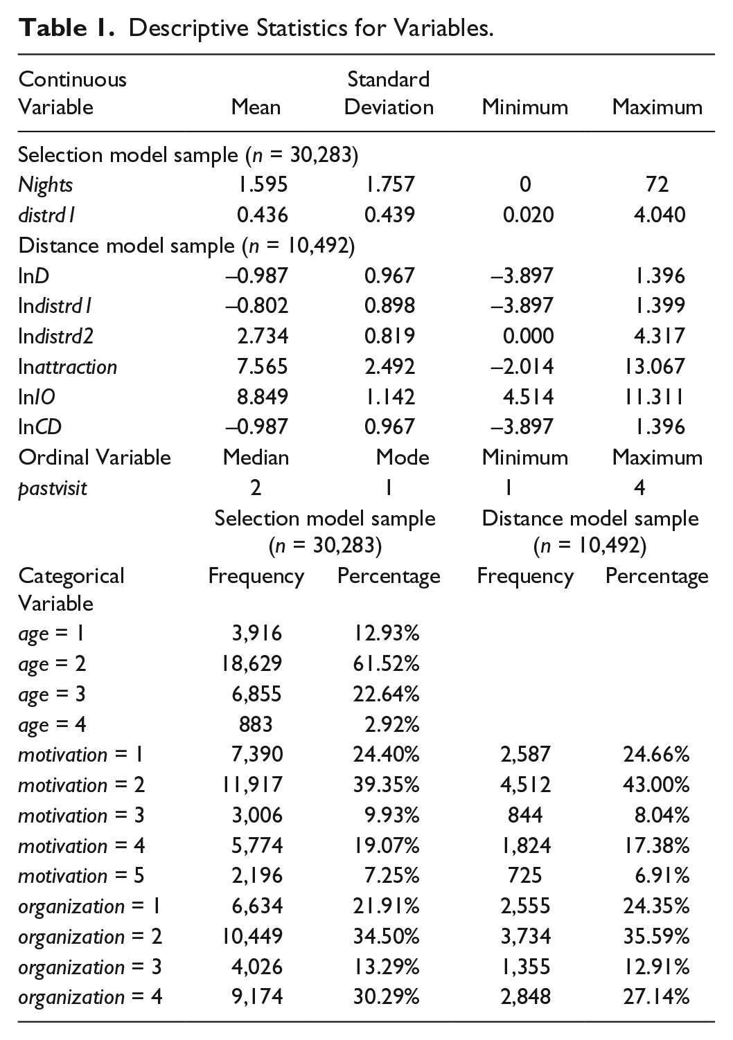
To make the explanation of the model estimation results more straightforward, our sample includes only those respondents whose first destination was the city where they were surveyed. Table 1 presents the descriptive statistics of the variables. Our sample is comprised of 30,283 Chinese domestic tourists to Jiangsu. The largest sample (5,587 respondents) was obtained in Nanjing (the capital of Jiangsu), whereas the smallest (973 respondents) was obtained in Suqian (Figure 1). Among all respondents in the sample, 10,492 intended to visit a subsequent destination after visiting Jiangsu (the previous destination). The sampled tourists had an average length of stay of 1.6 days and an average travel distance of 436 km to Jiangsu. The median value of the ordinal variable pastvisit is 2, and the modal value is 1. More specifically, 46.58% of tourists had not visited the destination before, and another 28.49% had visited only once before. For categorical variables, tourists between the ages of 25 and 44 (age = 2) dominated our sample. The distributions of organization and motivation are similar in the first-stage and second-stage equation samples. Around 40% of tourists traveled for sightseeing, while another 24% of tourists visited Jiangsu for vacation. Most tourists traveled with friends and relatives, and a substantial percentage of tourists were organized by affiliations or travel agencies. Table 2 presents the frequencies of 20 most-selected subsequent destinations from our sample, which account for 90.82% of destination choices. The results suggest that most of these destinations are either in Jiangsu or located in other provinces of the Yangtze River Delta area.

Table 1.

Descriptive Statistics for Variables.

Continuous Variable	Mean	Standard Deviation	Minimum	Maximum
Selection model sample (n = 30,283)
Nights	1.595	1.757	0	72
distrd1	0.436	0.439	0.020	4.040
Distance model sample (n = 10,492)
lnD	−0.987	0.967	−3.897	1.396
lndistrd1	−0.802	0.898	−3.897	1.399
lndistrd2	2.734	0.819	0.000	4.317
lnattraction	7.565	2.492	−2.014	13.067
lnIO	8.849	1.142	4.514	11.311
lnCD	−0.987	0.967	−3.897	1.396
Ordinal Variable	Median	Mode	Minimum	Maximum
pastvisit	2	1	1	4
	Selection model sample (n = 30,283)		Distance model sample (n = 10,492)
Categorical Variable	Frequency	Percentage	Frequency	Percentage
age = 1	3,916	12.93%
age = 2	18,629	61.52%
age = 3	6,855	22.64%
age = 4	883	2.92%
motivation = 1	7,390	24.40%	2,587	24.66%
motivation = 2	11,917	39.35%	4,512	43.00%
motivation = 3	3,006	9.93%	844	8.04%
motivation = 4	5,774	19.07%	1,824	17.38%
motivation = 5	2,196	7.25%	725	6.91%
organization = 1	6,634	21.91%	2,555	24.35%
organization = 2	10,449	34.50%	3,734	35.59%
organization = 3	4,026	13.29%	1,355	12.91%
organization = 4	9,174	30.29%	2,848	27.14%

Figure 1.

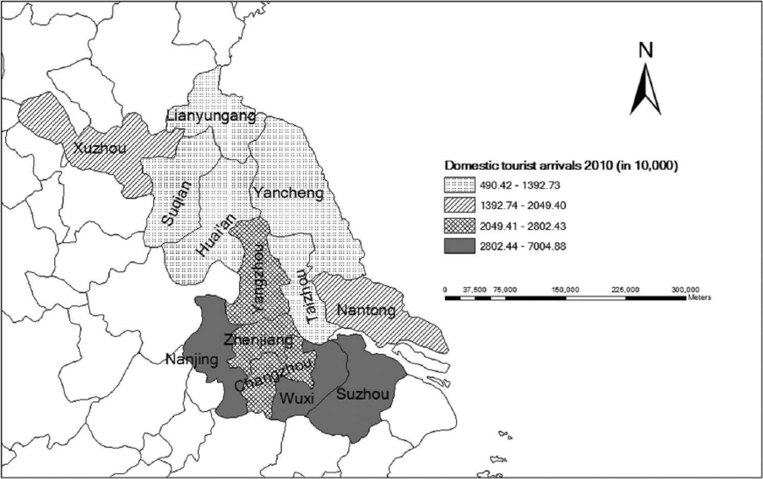
Location map of Jiangsu cities.

Figure 2.

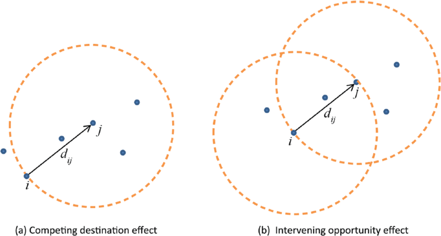
Geographic space of spatial structure effect.

Figure 3.

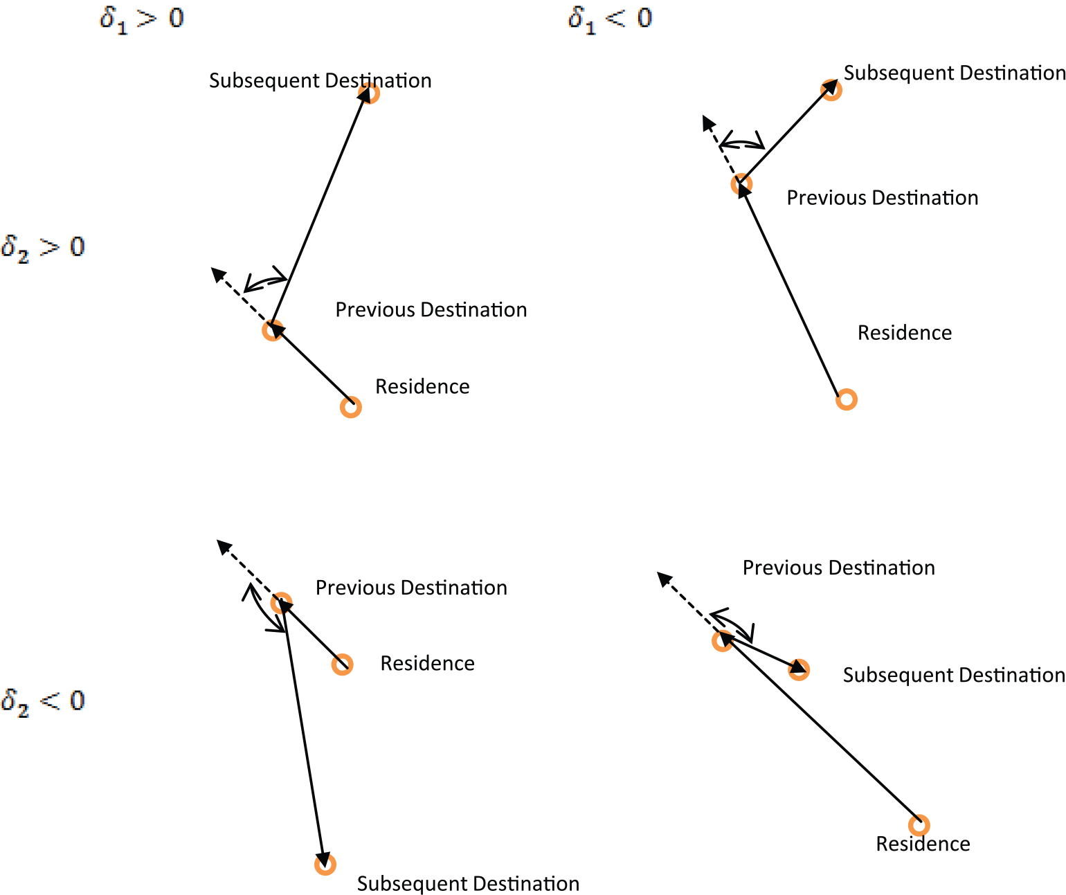
Geometric typology of multidestination travel based on model estimates.

Table 2.

Frequencies of 20 Most-Selected Subsequent Destinations.

Rank	Subsequent Destination	Frequency	Percentage	Cumulative Percentage
1	Shanghai^a	2,952	28.14	28.14
2	Nanjing^b	1,381	13.16	41.30
3	Suzhou^b	1,151	10.97	52.27
4	Wuxi^b	627	5.98	58.24
5	Hangzhou^a	553	5.27	63.52
6	Yangzhou^b	499	4.76	68.27
7	Changzhou^b	394	3.76	72.03
8	Lianyungang^b	385	3.67	75.70
9	Xuzhou^b	232	2.21	77.91
10	Nantong^b	218	2.08	79.98
11	Zhenjiang^b	186	1.77	81.76
12	Huai’an^b	155	1.48	83.23
13	Huangshan	154	1.47	84.70
14	Beijing	143	1.36	86.07
15	Qingdao	110	1.05	87.11
16	Taizhou^b	99	0.94	88.06
17	Jinan	85	0.81	88.87
18	Suqian^b	72	0.69	89.55
19	Yancheng^b	70	0.67	90.22
20	Hefei	63	0.60	90.82
Total		10,492		100.00

Cities in the Yangtze River Delta area.

Jiangsu cities.

Tourism Spillover Index and GIS Visualization

After obtaining the estimates for the two-stage model, we constructed a tourism spillover index (TSI) to evaluate the magnitude of spillovers arising from multidestination travel. The TSI reflects the total potential of tourists traveling to a particular destination j after visiting a previous destination i, and is defined as follows:

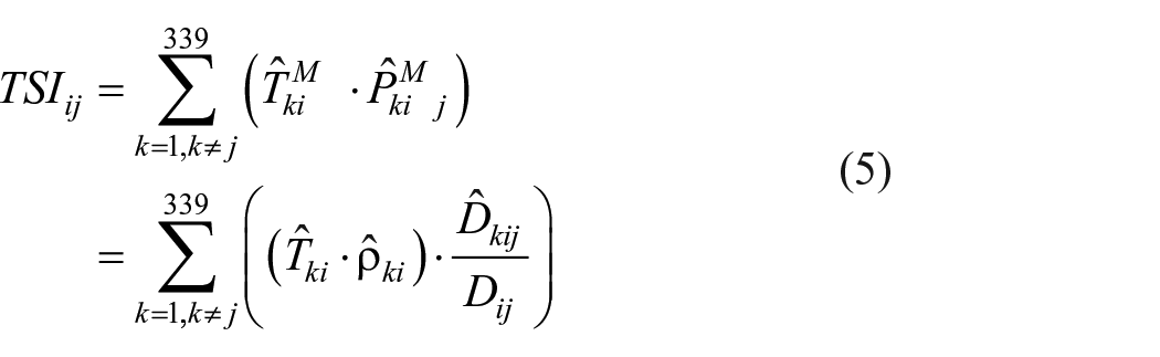
\begin{matrix} T S I_{i j} = \sum_{k = 1, k \neq j}^{339} ({\hat{T}}_{k i}^{M} {\hat{P}}_{k i j}^{M}) \\ = \sum_{k = 1, k \neq j}^{339} (({\hat{T}}_{k i} \cdot {\hat{ρ}}_{k i}) \cdot \frac{{\hat{D}}_{k i j}}{D_{i j}}) \end{matrix}

(5)

where k indexes the tourist’s origin as a prefectural city in mainland China (k = 1, …, 339; k ≠ j). It is assumed that the overall magnitude of a spillover is the sum of those spillovers contributed by tourists from all possible origins. The index is a sum of the products of two terms. The first term, ${\hat{T}}_{k i}^{M}$ ,denotes the total tourist arrivals (in 10,000s) from origin k to a previous destination i who will continue to travel to any subsequent destination region. More specifically, we wrote out ${\hat{T}}_{k i}^{M} = {\hat{T}}_{k i} \cdot {\hat{ρ}}_{k i}$ ,where ${\hat{T}}_{k i}$ represents the number of tourists from origin k to a previous destination i, and ${\hat{ρ}}_{k i}$ denotes the probability of these tourists continuing to travel to a subsequent destination. We used a gravity model to predict the term ${\hat{T}}_{k i}$ (Tadesse and White 2012), and calculated the term ${\hat{ρ}}_{k i j}$ based on the estimates from Equation 1. The second term ${\hat{P}}_{k i j}^{M}$ in Equation 5 reflects the “intensity” level of multidestination travel for tourists from origin k leaving destination i, conditional on the level of attractions and spatial structure effect (CD and IO effects) offered by destination region j as a subsequent destination. We expressed ${\hat{P}}_{k i j}^{M} = {\hat{D}}_{k i j} / D_{i j}$ , where ${\hat{D}}_{k i j}$ represents the predicted distance from the second-stage distance equation (Equation 2) for a tourist from origin k leaving the previous destination i, conditional on the same level of attractions and spatial structure effect (CD and IO) offered by destination j as a subsequent destination; $D_{i j}$ is the actual distance between destinations i and j. The ratio between ${\hat{D}}_{k i j}$ and $D_{i j}$ reflects the capability of a tourist from origin k to overcome distance barriers to travel to destination j as a subsequent destination region after leaving destination i. If the tourist is willing to travel a long distance to a subsequent destination k given its attractiveness and spatial structure, this destination is likely to receive a large proportion of multidestination travelers leaving a previous destination i, and ${\hat{P}}_{k i j}^{M}$ should be high when other factors are held constant. Note that ${\hat{P}}_{k i j}^{M}$ does not necessarily fall between 0 and 1, and therefore, it is different from a “probability” or “likelihood” of multidestination travel. Because our two-stage model incorporates non-i.i.d. error terms and uses log distance as the dependent variable, the conditional expectation of distance is complicated, and is derived as follows (see the proof in the Appendix):

\begin{array}{l} E [D | \ln D observed] \\ = \exp (W^{'} ξ + \frac{1}{2} (1 - ρ) σ^{2} + \frac{1}{2} ρ^{2} σ^{2}) \cdot \frac{Φ (Z^{'} γ - ρ σ)}{Φ (Z^{'} γ)} \end{array}

(6)

where $Φ (\cdot)$ denotes the cumulative density function of the standard normal distribution; $W = [\ln d i s t r d, \ln d i s t r d, X]$ ; $ξ = {(δ_{1}, δ_{2}, β^{'})}^{'}$ . By substituting the estimates into the conditional expectation (Equation 6), the predicted distance ${\hat{D}}_{k i j}$ becomes

{\hat{D}}_{k i j} = \exp (W^{'} \hat{ξ} + \frac{1}{2} (1 - \hat{ρ}) {\hat{σ}}^{2} + \frac{1}{2} {\hat{ρ}}^{2} {\hat{σ}}^{2}) \cdot \frac{Φ (Z^{'} \hat{γ} - \hat{ρ} \hat{σ})}{Φ (Z^{'} \hat{γ})}

(7)

Considering that tourism is an essentially spatial phenomenon involving the movement of tourists from origins to destinations, geographic information system (GIS) applications have become prominent decision-making tools in tourism planning, trip modeling, and destination management (Chancellor and Cole 2008). As powerful spatial visualization tools, GIS applications have been employed to understand the spatial-temporal patterns of multidestination trips (Wu and Carson 2008). Another powerful GIS application in tourism is geo-demographic marketing analysis: the delineation of geographic market areas based on distance, user and site characteristics, and demographic profiles, as well as the evaluation of market potential for different types of destination products (Feng and Morrison 2002; Miller 2008; Chancellor 2012; Chancellor and Cole 2008). For example, Rutherford, Kobryn, and Newsome (2015) presented a GIS application to assess potential areas for geo-tourism based on tourism access and other factors. To visualize the TSI for each destination region, we applied GIS techniques to present the calibrated TSI values as either spillover generators or receivers. By understanding the patterns revealed in the GIS outputs, DMOs and local tourism authorities are able to better identify potential regions for collaboration and specific market segments to target as multidestination tourists to their regions (Beritelli, Bieger, and Laesser 2014).

Empirical Results

Two-Stage Distance-Based Model

Table 3 presents the estimation results of the two-stage distance-based models. Model 1 is fitted by using all observations. The results from the first-stage selection equation show that out of the three dummy variables for age, only age = 2 is estimated to be statistically significant. Its positive coefficient suggests that compared to younger tourists, those between the ages of 25 and 44 are likely to continue their trips to a subsequent destination. Moreover, nights is estimated to be insignificant. The negative estimate of pastvisit and the positive estimate of distrd1 suggest that first-time and long-haul tourists have a high propensity to travel to a subsequent destination. These findings can be explained by the fact that first-time tourists tend to be more novelty seeking (Tideswell and Faulkner 2003) and long-haul tourists are likely to maximize their utility associated with high travel costs (Yang, Fik, and Zhang 2013). Regarding travel organization patterns and motivations, we find that tourists organized by affiliations (organization = 1) and leisure/vacation and sightseeing tourists (motivation = 1 and 2) are more likely to continue their travel after visiting a destination than other tourists.

Table 3.

Estimation Results of Empirical Models.

	Model 1	Model 2	Model 3	Model 4	Model 5	Model 6	Model 7	Model 8	Model 9	Model 10
	All data	motivation=1	motivation=2	motivation=3	motivation=4	motivation=5	organization=1	organization=2	organization=3	organization=4
First-stage selection equation
age = 2	0.0493**	−0.127***	0.0804**	0.202**	0.00933	0.265***	−0.139**	0.167***	0.00611	0.0588
	(0.025)	(0.038)	(0.033)	(0.090)	(0.108)	(0.091)	(0.062)	(0.039)	(0.039)	(0.044)
age = 3	0.0223	−0.108**	0.0675*	0.0931	−0.0183	0.170*	−0.127*	0.159***	−0.0214	0.0571
	(0.028)	(0.043)	(0.040)	(0.092)	(0.102)	(0.099)	(0.066)	(0.045)	(0.049)	(0.050)
age = 4	−0.0586	−0.123*	−0.0775	−0.197	−0.264	0.129	−0.270***	0.0103	−0.0711	0.0436
	(0.051)	(0.073)	(0.080)	(0.152)	(0.227)	(0.144)	(0.098)	(0.091)	(0.097)	(0.105)
nights	−0.00683	0.0520***	−0.0382***	−0.0453**	−0.0183	0.00388	0.0152*	−0.0598***	0.0393**	0.0106
	(0.005)	(0.013)	(0.010)	(0.021)	(0.014)	(0.018)	(0.008)	(0.011)	(0.019)	(0.009)
organization = 2	−0.0976***	−0.0179	−0.221***	−0.354***	0.0571	−0.194**
	(0.023)	(0.043)	(0.038)	(0.090)	(0.062)	(0.078)
organization = 3	−0.221***	−0.396***	−0.245***	−0.209	0.599***	−0.156
	(0.028)	(0.051)	(0.043)	(0.140)	(0.091)	(0.102)
organization = 4	−0.204***	−0.179***	−0.250***	−0.510***	−0.104***	−0.260***
	(0.022)	(0.045)	(0.041)	(0.093)	(0.040)	(0.071)
pastvisit	−0.0701***	−0.0185	−0.00597	−0.135***	−0.143***	−0.225***	−0.0956***	−0.129***	0.0284	−0.0490***
	(0.008)	(0.013)	(0.013)	(0.025)	(0.019)	(0.028)	(0.015)	(0.013)	(0.032)	(0.014)
distrd1	0.609***	0.457***	0.866***	0.456***	0.464***	0.285***	0.564***	0.671***	0.502**	0.490***
	(0.019)	(0.051)	(0.038)	(0.057)	(0.039)	(0.059)	(0.041)	(0.035)	(0.214)	(0.033)
motivation = 2	0.0932***						0.165***	−0.0806***	0.318***	0.105***
	(0.019)						(0.048)	(0.031)	(0.049)	(0.037)
motivation = 3	−0.179***						0.0837	−0.283***	0.280**	−0.270***
	(0.030)						(0.090)	(0.045)	(0.132)	(0.052)
motivation = 4	−0.168***						−0.203***	−0.214***	0.682***	−0.188***
	(0.026)						(0.044)	(0.064)	(0.092)	(0.044)
motivation = 5	−0.0818**						−0.00381	−0.246***	0.165*	−0.139**
	(0.033)						(0.064)	(0.064)	(0.090)	(0.056)
constant	−0.421***	−0.398***	−0.452***	−0.158	−0.377***	−0.172	−0.241***	−0.329***	−0.961***	−0.638***
	(0.036)	(0.054)	(0.053)	(0.125)	(0.114)	(0.118)	(0.074)	(0.052)	(0.170)	(0.053)
Second-stage distance equation
lndistrd1 (δ₁)	−0.0190***	−0.0747***	−0.0332***	0.00737	−0.00906	−0.000414	−0.0521***	−0.0259***	−0.104***	−0.0175*
	(0.006)	(0.009)	(0.008)	(0.024)	(0.021)	(0.016)	(0.010)	(0.009)	(0.026)	(0.009)
lndistrd2 (δ₂)	0.0723***	0.0647***	0.106***	0.0418**	0.0485***	0.0246	0.0219**	0.0936***	0.0407	0.0949***
	(0.006)	(0.011)	(0.009)	(0.017)	(0.011)	(0.017)	(0.009)	(0.010)	(0.035)	(0.010)
lnattraction	0.162***	0.130***	0.189***	0.145***	0.127***	0.131***	0.149***	0.195***	0.103	0.126***
lnattraction	(0.004)	(0.013)	(0.007)	(0.013)	(0.009)	(0.012)	(0.007)	(0.007)	(0.073)	(0.008)
lnIO	−0.279***	−0.272***	−0.272***	−0.279***	−0.281***	−0.292***	−0.278***	−0.276***	−0.276***	−0.277***
	(0.001)	(0.003)	(0.002)	(0.005)	(0.003)	(0.005)	(0.003)	(0.003)	(0.004)	(0.003)
lnCD	0.0184***	−0.0156	−0.00454	0.0704***	0.0431***	0.0328***	0.0388***	0.00494	−0.0691***	0.0214***
	(0.003)	(0.018)	(0.005)	(0.011)	(0.008)	(0.012)	(0.010)	(0.005)	(0.017)	(0.007)
motivation = 2	0.0161**						−0.0205	0.0226**	−0.131***	0.00844
	(0.007)						(0.019)	(0.011)	(0.038)	(0.014)
motivation = 3	−0.0110						−0.0251	0.00509	−0.114	−0.0543**
	(0.013)						(0.034)	(0.018)	(0.083)	(0.024)
motivation = 4	−0.00624						0.0517***	−0.0445**	−0.234**	−0.0413**
	(0.009)						(0.018)	(0.023)	(0.120)	(0.016)
motivation = 5	−0.00950						−0.0281	−0.00882	−0.0813	−0.0237
	(0.012)						(0.024)	(0.023)	(0.068)	(0.021)
organization = 2	0.0177**	0.00950	0.00885	0.0522	−0.0331	0.0622**
	(0.008)	(0.020)	(0.012)	(0.040)	(0.023)	(0.030)
organization = 3	0.00226	0.134***	−0.0219	0.0125	0.0706	0.0397
	(0.011)	(0.028)	(0.014)	(0.062)	(0.057)	(0.037)
organization = 4	0.0102	0.0718***	−0.00736	0.0297	−0.000623	0.0619**
	(0.009)	(0.023)	(0.014)	(0.053)	(0.018)	(0.029)
constant	−0.276***	0.403*	−0.211***	−0.686***	−0.390***	−0.176	−0.223**	−0.280***	1.179**	−0.246***
	(0.039)	(0.215)	(0.051)	(0.140)	(0.140)	(0.128)	(0.104)	(0.058)	(0.497)	(0.083)
ρ	−0.00867	−0.937***	0.178***	−0.128	−0.0270	−0.400*	−0.842***	0.119*	−0.985**	0.226
σ	0.279***	0.466***	0.273***	0.298***	0.266***	0.280***	0.367***	0.273***	0.528***	0.290***
N	30283	7390	11917	3006	5774	2196	6634	10449	4026	9174
AIC	40432.3	10002.6	15929.4	3746.6	7243.8	2806.0	8881.1	13788.1	5247.0	11944.7
BIC	40673.5	10147.6	16084.5	3872.8	7383.7	2925.6	9037.5	13955.0	5391.9	12108.5

Note: Robust standard errors are presented in parentheses. Asterisks indicate significance at the *0.10, **0.05, and ***0.01 levels. AIC = Akaike information criterion; BIC Bayesian information criterion.

For the results from the second-stage distance equation, $δ_{1}$ is estimated to be negative, while $δ_{2}$ is positive. A negative estimate of $δ_{1}$ suggests that long-haul tourists tend to travel to a subsequent destination that is closer to the previous one if they opt to continue the tour. A positive estimate of $δ_{2}$ shows that tourists tend to pick a subsequent destination that is farther away from their residences than the previous destination. Therefore, the spatial movement pattern resembles the one shown in the upper right of the graph depicted in Figure 3. Regarding the estimates of other independent variables explaining travel distance, lnattraction is significant and positive, indicating that the abundance of tourist attractions entices tourists to travel a longer distance to a subsequent destination. Unsurprisingly, the two spatial structure variables are also estimated to be statistically significant. A negative estimate of lnIO illustrates that the existence of substitutable destinations located between the previous and subsequent destinations impedes tourist movements, whereas a positive estimate of lnCD indicates the agglomeration effect of destinations to attract multidestination travelers. Moreover, it is found that tourists traveling with friends and relatives (organization = 2) and sightseeing tourists (motivation = 2) travel longer distances than other tourists to a subsequent destination. Lastly, ρ is estimated to be insignificant, indicating that the first-stage and second-stage equations are not significantly intercorrelated.

To further investigate the role of different travel motivations, we estimated separate models to decipher multidestination travel patterns. The results of Models 2 through 6 are shown in Table 3. In the first-stage selection equation, some results are similar across different the models, such as the estimates of distrd1 and organization. However, the estimated coefficients associated with some independent variables vary greatly across different models. For instance, according to the estimates of age, young tourists less than 24 years of age (age = 1) who travel for leisure/vacation purposes (motivation = 1) are more likely to travel to a subsequent destination (Model 2), whereas their counterparts who travel for sightseeing purposes (motivation = 2) are less likely to do so (Model 3). The number of nights spent at a previous destination also influences the subsequent travel decision for tourists traveling for leisure/vacation (Model 2), sightseeing (Model 3), and VFR (Model 4) purposes. Because of time constraints, a longer stay at a previous destination is associated with a lower probability of travel to another destination (Yang, Fik, and Zhang 2013); hence, a negative coefficient is expected (Koo, Wu, and Dwyer 2010), which is consistent with the results in Models 3 and 4. One possible reason for the positive coefficient of nights in Model 2 is that, for vacationing tourists, a longer duration at the first destination may indicate a large time budget for the entire trip, which enables them to travel to other destinations. The number of past visits is found to determine the likelihood of subsequent travel for tourists traveling for VFR (motivation = 3), business/conference reasons (motivation = 4), and other motivations (motivation = 5) (Models 4–6). For the estimates of the second-stage distance equation, $δ_{1}$ is significant and negative in Models 2 and 3, while $δ_{2}$ is consistently significant and positive in Models 2–5. As suggested by the positive and significant estimate of lnattraction in the models, we find that tourist attractions play a vital role in enticing tourists to travel further, and this factor is particularly more important for sightseeing tourists (Model 3). This result can be explained by the fact that the attraction index we proposed incorporates more sightseeing attractions. The magnitudes of the lnIO estimates are quite close in Models 2–6, showing that the effect of intervening opportunities is robust to tourists with different motivations. In Models 4–6, lnCD is consistently positive and significant, and its estimate is found to be considerably larger for VFR and business/conference tourists (Models 4 and 5), suggesting that the advantage of agglomeration economies is more substantial for these types of tourists. Lastly, the estimate of ρ is nonsignificant in Models 4–6, indicating that for tourists traveling for VFR, business/conference, and other purposes, multidestination travel decisions at the two stages are independent.

Models 7–10 in Table 3 provide estimates for subsamples of tourists with different travel organization patterns. The estimates of the first-stage selection equation vary greatly across different models. The age estimates suggest that young tourists less than 24 years of age (age = 1) who are organized by affiliations (organization = 1) are more likely to travel to a subsequent destination than others, whereas their counterparts who travel with friends and relatives (organization = 2) are less likely to continue their trips. Although nights is estimated to be positive in most models, it is found to be negative in Model 8 for tourists traveling with friends and relatives. In the second-stage distance equation, the negative $δ_{1}$ and positive $δ_{2}$ estimates are significant in most of the four models. The estimates of lnattraction and lnIO are also quite similar in the different models. The competing destination measure, lnCD is estimated to be significant and negative in Model 9 for tourists organized by travel agencies, suggesting a high level of cross-destination competition for tourists in this segment. Sightseeing tourists (motivation = 2) who are organized by travel agencies and traveling alone tend to travel further to a subsequent destination than others (Models 9 and 10), whereas their counterparts who are traveling with friends and relatives tend to travel a shorter distance to the next destination (Model 8).

Tourism Spillover Index

We calibrated the TSI for each prefectural city in China based on a particular Jiangsu city as the spillover generator from Equation 5. We used a Poisson gravity model to predict ${\hat{T}}_{k i}$ (the number of tourist arrivals from origin k for a particular destination i) (Tadesse and White 2012). The Poisson regression model is estimated to be:

l n T_{k i} = \ln T_{i} - 8.832 + 1.070 * \ln G D P_{k} - 0.764 * \ln d_{k i}

where k and i index the origin and destination (more specifically, the previous destination in a multidestination trip), respectively. $T_{i}$ denotes the total number of tourist arrivals to destination i; $G D P_{k}$ measures the total gross domestic product of origin k; and $d_{k i}$ represents the geographic distance from k to i. All estimated coefficients are statistically significant at the 0.01 level, and the pseudo-R-squared is 0.696. For a particular spillover generator, which is a previous destination in a multidestination travel itinerary, we can calculate the TSI for all other cities to evaluate their potential to attract multidestination travelers after leaving that previous destination. We generated 13 maps to demonstrate the TSI of each Chinese prefectural city to attract spillovers from each of the 13 Jiangsu cities, respectively.

Because of space limitations, Figure 4 presents four of the 13 TSI maps, which visualize the spillover potential to all Chinese prefectural cities from four Jiangsu cities: Nanjing, Suzhou, Xuzhou, and Yancheng (highlighted by arrows). Nanjing, the capital of Jiangsu Province, is the largest city and the second largest tourist receiver in the province. Suzhou received the largest number of domestic tourists in 2010. These two cities are located in the southern part of the province. The other two cities, Xuzhou and Yancheng, are located in the northwestern and northeastern parts of the province, respectively. These maps show that TSI generally declines with distance from the spillover generator. As indicated by the large value of TSI, neighboring cities are likely to receive more spillovers. For Nanjing and Xuzhou, most cities with high TSI values are clustered nearby. For Suzhou, two clusters of high TSI values are found: one covers cities nearby, and the other consists of several cities in the northern part of Jiangsu Province and the southern part of Shandong Province. For Yancheng, the city generating few tourism spillovers, only a few neighboring cities are characterized by relatively high TSI values as potential spillover recipients. Lastly, some distant cities from the spillover generators are characterized by high TSI values, such as Beijing, Chongqing, Wuhan, and Luoyang, because of the abundant tourist resources offered there.

Figure 4.

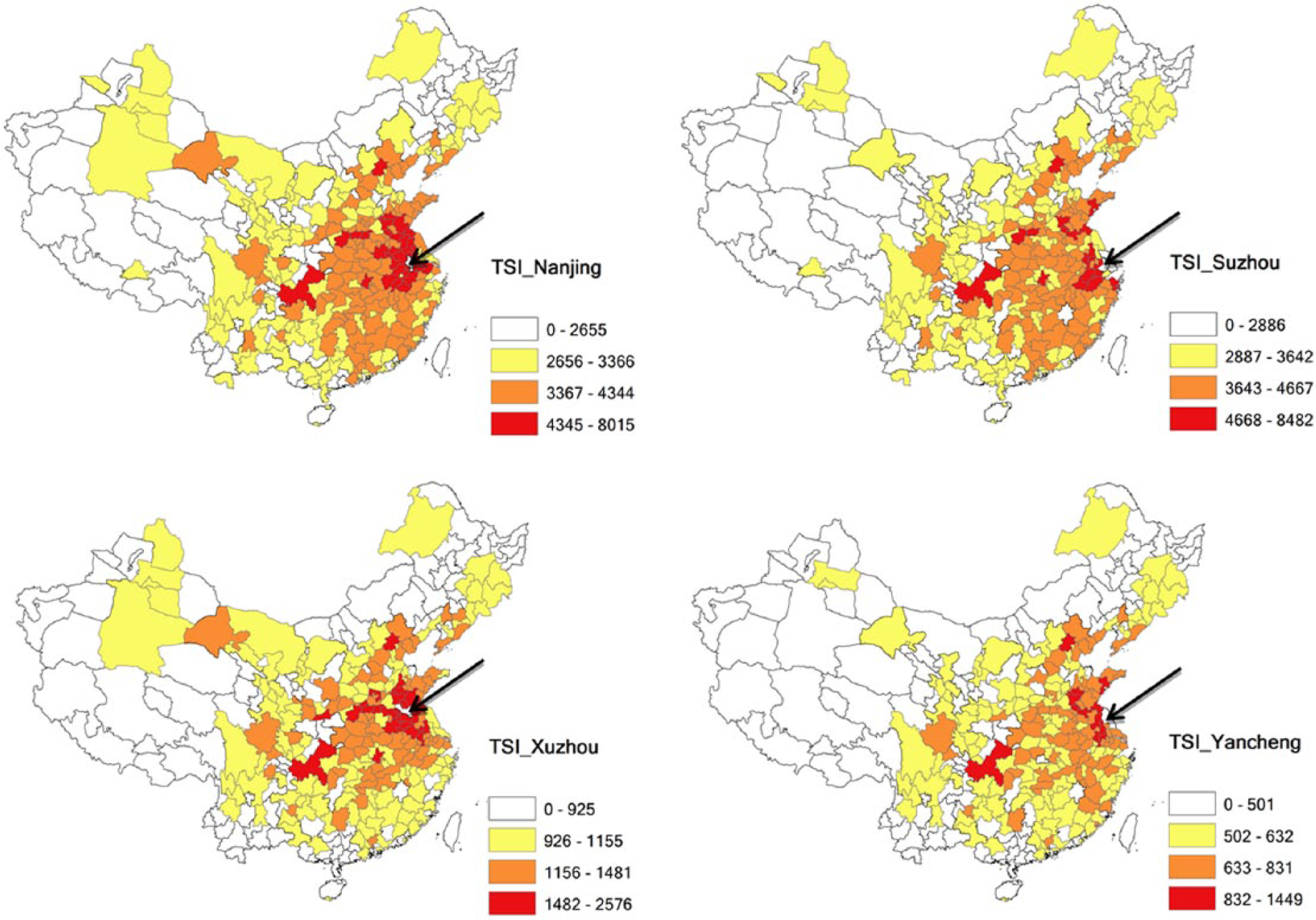
Tourism spillover index values of destinations from four Jiangsu cities.

We further obtained the TSI values for different types of tourists according to the estimates from Models 2–10 in Table 3. Figure 5 presents the TSI maps for spillovers generated by tourists with different organization patterns who visited Suzhou (highlighted by the arrow), the most popular domestic tourist destination in Jiangsu. In general, the TSI values decay with distance to Suzhou. Compared to their counterparts in Figure 4, those cities with high TSI values for tourists traveling with friends and relatives (organization = 2) and alone (organization = 4) are relatively scattered over the space, suggesting that many distant cities from Suzhou are also likely to benefit from spillovers generated by the multidestination travel of these two types of tourists. For tourists organized by affiliations (organization = 1), only a few nearby cities are likely to receive substantial spillovers from Suzhou; whereas for tourists organized by travel agencies (organization = 3), the generated spillovers from Suzhou are quite substantial, covering a broad geographic area.

Figure 5.

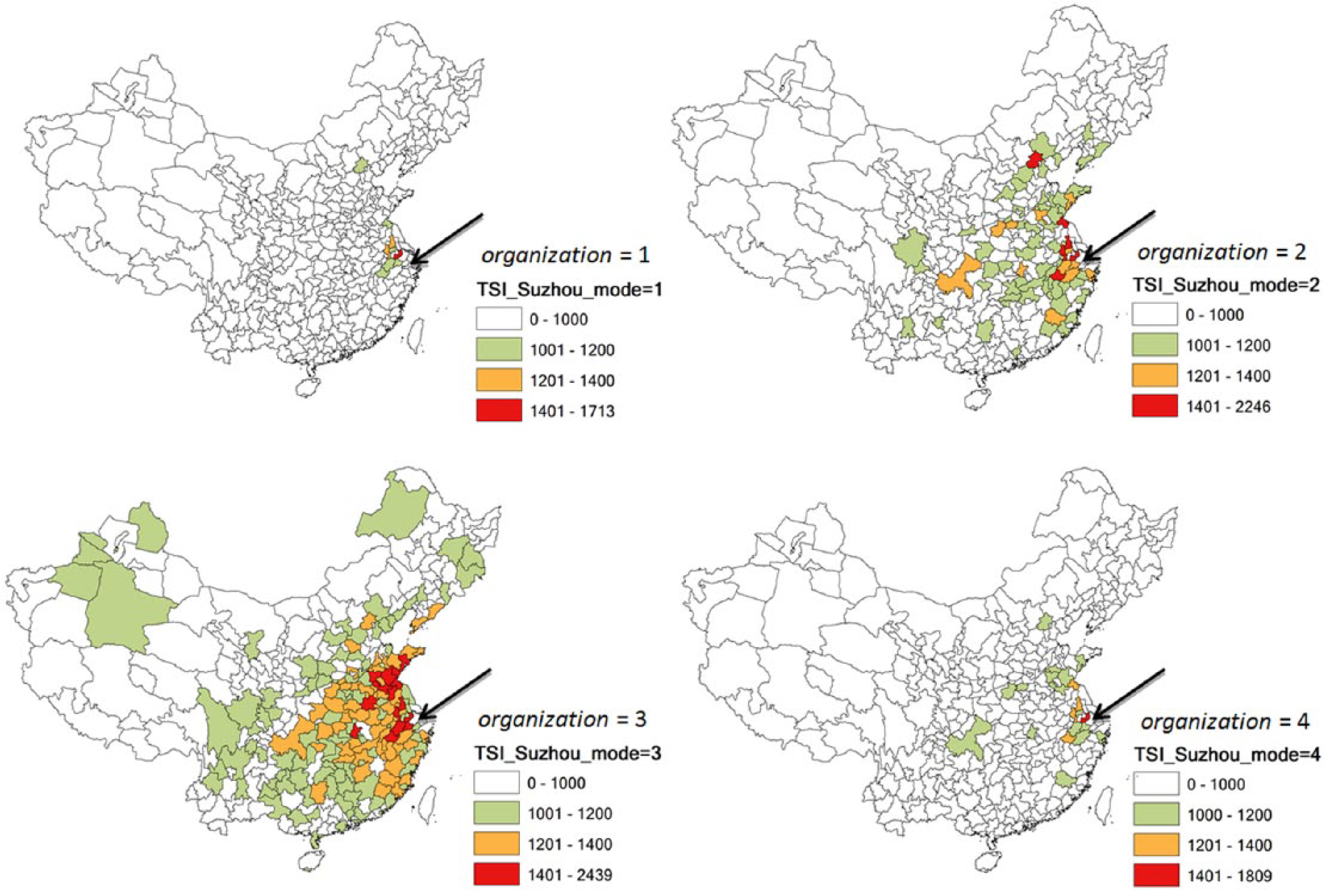
Tourism spillover index values from Suzhou with different organization patterns.

For a specific subsequent destination as a potential spillover receiver, the TSI provides important information on selecting potential collaborators for tourism marketing. We selected Wenzhou, a prefectural city in Zhejiang Province, to illustrate the analysis of TSI for a single spillover receiver. Table 4 presents the TSI values of Wenzhou as a spillover receiver based on 13 different Jiangsu cities as spillover generators. For the spillovers from all tourists, Suzhou contributes most to spillovers, followed by Nanjing and Wuxi. Furthermore, we were able to identify the largest spillover generators based on tourist types. Although Suzhou still produces the largest spillovers from tourists traveling for leisure/vacation (motivation = 1) or VFR (motivation = 3) purposes and those traveling through affiliations (organization = 1), travel agencies (organization = 3) and alone (organization = 4), Nanjing is the largest spillover generator for sightseeing tourists (motivation = 2), Wuxi for business/conference tourists (motivation = 4), and Changzhou for tourists with other motivations (motivation = 5).

Table 4.

Tourism Spillover Index for Wenzhou, Zhejiang Province as a Spillover Receiver.

Spillover Generator	All Data	Motivation					Organization
Spillover Generator	All Data	1	2	3	4	5	1	2	3	4
Nanjing	3726.46	1221.73	1744.74	159.35	132.40	111.81	492.38	1351.47	657.13	681.86
Wuxi	3182.90	835.91	1011.75	157.15	542.05	201.43	781.46	681.44	588.93	873.24
Xuzhou	1028.68	157.27	199.29	71.14	310.14	66.27	446.42	188.70	73.69	214.71
Changzhou	1609.97	389.90	334.95	92.01	331.70	224.71	395.17	377.67	491.56	339.40
Suzhou	4501.90	1841.55	1535.56	194.88	458.10	218.54	893.90	1174.34	1345.07	972.42
Nantong	965.36	253.82	328.80	55.23	133.37	61.13	201.64	224.01	154.28	272.58
Lianyungang	719.61	227.37	231.12	50.08	65.88	59.81	127.28	173.60	271.67	146.15
Huai’an	634.33	174.03	194.71	55.24	96.59	16.43	322.38	134.41	128.19	53.44
Yancheng	610.34	176.78	93.44	61.43	114.33	73.98	196.37	117.85	104.69	144.21
Yangzhou	1458.75	977.48	347.84	62.80	119.72	44.81	610.90	165.47	383.08	349.38
Zhenjiang	1505.94	1376.96	292.38	58.50	37.76	27.54	318.87	113.28	1018.12	414.36
Taizhou	601.05	223.42	187.70	21.60	84.38	34.71	191.98	62.91	476.44	75.61
Suqian	261.38	106.77	70.62	13.30	37.64	12.55	102.03	48.31	92.11	35.18

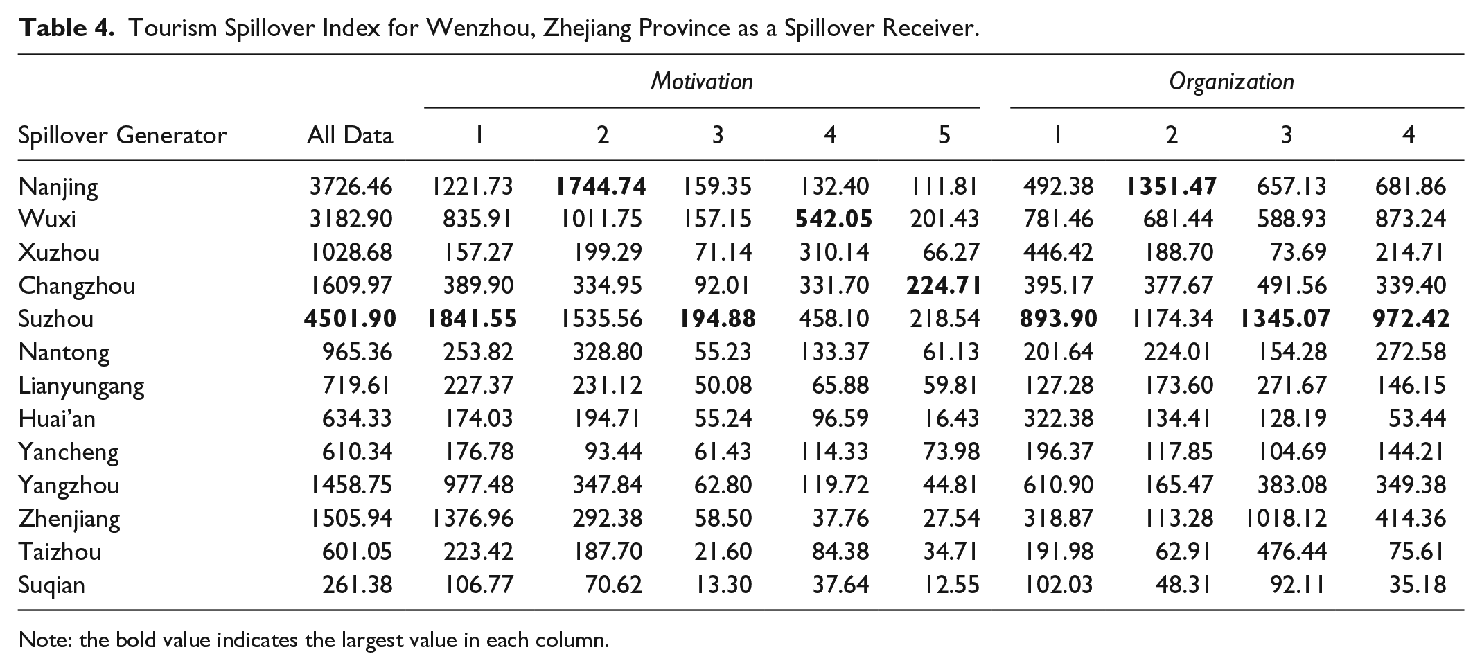
Note: the bold value indicates the largest value in each column.

Conclusion

In this article, we proposed a two-stage distance-based model to investigate the spatial patterns of multidestination trips. Using the first-stage selection equation, we found that a tourist’s decision to travel to a subsequent destination is determined by the organization pattern, travel motivation, and travel distance from his or her residence to the destination, as well as length of stay and number of past visits to a previous destination. Using the second-stage distance equation, we found the travel distance from the previous to the subsequent destination to be associated with the popularity of tourist attractions, tourists’ organization patterns and motivations, and spatial structure factors (including CD and IO effects). The competing destination effect contributes to an agglomeration force to entice more tourists to travel further to a particular subsequent destination, whereas the intervening opportunities effect impedes multidestination travel when substitutable destinations are located between two destinations. It can be argued that these two distinct spatial structure effects should be accounted for if acceptable parameter estimates for other independent variables are to be found in the second-stage modeling process. The importance of distance-based variables cannot be overlooked based on the geometric typology in Figure 2. Note that it was shown that long-haul tourists travel to subsequent destinations that are closer to the previous one if they opt to continue the tour, whereas generally tourists pick a subsequent destination that is farther away from home than the previous destination.

Our study contributed to the current knowledge of tourist flow analysis in several ways. First, we proposed the two-stage distance-based model to unveil factors determining multidestination travel, and this model was theoretically rooted in one of the most popular theories explaining tourist flows: spatial interaction theory. Second, the geometric typology embedded in the distance-based model provides a concise but wide-ranging insight on the multidestination patterns. Compared to conventional qualitative analysis (Lew and McKercher 2006), our quantitative investigation is able to conduct significance test to discriminate geometric typologies at an aggregate level, and estimated coefficients associated with different typology patterns can be compared and evaluated. Third, we developed a TSI based on the estimation results of the two-stage distance-based model and demonstrated the usefulness of this index in calibrating the market potential for multidestination travelers and targeting potential destination partners for strategical joint-marketing campaigns of different market segments. Last but not least, even though our analysis incorporated only two destinations, the model is flexible in embracing more destinations by assuming the multidestination travel is a Markov-chain process, in which the transition probability of chain states hinges on the probability in the first-step probit equation of our model (Xia, Zeephongsekul, and Packer 2011).

Our research findings provide several important implications for DMOs that could help them internalize spatial spillovers from multidestination tourists. First, as improvements are made to transportation infrastructure and the popularity of self-driving increases, more and more Chinese tourists are likely to make/change destination decisions during their trips. Therefore, DMOs could launch marketing campaigns to attract more tourists by focusing on segments composed of people who are more likely to travel to a subsequent destination. According to the results from our first-stage equation, long-haul tourists are associated with a high probability of multidestination travel; thus, DMOs should increase destination exposure in areas frequented by large numbers of these tourists, such as railway stations and airports. Second, among tourists in different age groups, multidestination travel decisions are driven by different purposes. For example, to encourage multidestination travel among young tourists, vacation products should be the focus, whereas sightseeing products are more likely to entice middle-aged tourists. Third, our results indicate that the popularity of tourist attractions is not a significant factor explaining the travel distance to a subsequent destination for tourists organized by travel agencies. Therefore, for destinations with limited attraction endowments, DMOs are encouraged to work closely with travel agencies to increase the market share of multidestination travelers. Lastly, the competing destination effect was found to be positive and substantial for the VFR segment. Therefore, to leverage this agglomeration effect with neighboring destinations, we recommend that DMOs and attractions offer deep discounts to residents from neighboring cities to nurture this market.

The geometric typology pattern presented in Figure 3 enables DMOs to better understand the spatial movements of tourists and the market potentials of their destinations. Based on the estimates of the two-stage distance model, we proposed a TSI to estimate the potential of a destination to receive spillover benefits from other destinations triggered by multidestination travelers. Therefore, for a particular destination, a myriad of potential collaborators can be found based on the TSI values from other destinations. Implementing a marketing campaign targeting multidestination travelers by promoting an additional trip or side trip requires less effort than marketing a location as a primary or gateway destination, resulting in a higher return on investment. Spillover analysis could help tourism planners and stakeholders understand how tourists move among multiple destinations and recognize destination linkages from a demand perspective, which is useful in identifying potential opportunities for marketing collaboration among different DMOs for the purpose of attracting multidestination travelers. Moreover, those destinations should initiate strategic plans to bundle attractions and activities to augment their overall attractiveness by increasing the gravity effect to entice tourists, ultimately contributing to a competitive advantage for tourism growth (Chancellor 2012). Furthermore, the proposed TSI embraces a flexible framework to integrate additional high-frequency big data sources, such as geo-tagged social media data and cell phone roaming data (Pan and Yang 2016), to monitor and predict the multidestination flow patterns in a real-time fashion.

Several limitations may temper the generalizability of our results. First, the definition of domestic tourist varies across different countries; therefore, our results based on a Chinese sample may not be applicable in other countries. Second, because of data unavailability, we did not investigate the multidestination travel patterns of special-interest tourists such as adventure tourists, eco-tourists, and cultural tourists, which may differ from those of mass tourists. Third, we did not incorporate temporal patterns of multidestination travel; a more comprehensive spatial-temporal analysis of travel patterns deserves further research efforts. In our estimation results, several models have an insignificant ρ value, and further research efforts can be carried out to investigate its theoretic underpinning. Our proposed TSI is able to capture the overall spillover potential for a destination by summing the TSI values over all possible spillover generators. Therefore, in the future, researchers can estimate a two-stage distance-based model using data from a nationwide sample to calculate overall TSI. We also recommend that researchers utilize various permutation methods to calculate confidence intervals for the calibrated TSI values in future work.

Footnotes

Appendix

Declaration of Conflicting Interests

The author(s) declared no potential conflicts of interest with respect to the research, authorship, and/or publication of this article.

Funding

The author(s) disclosed receipt of the following financial support for the research, authorship, and/or publication of this article: The authors are grateful to the Ministry of Education, the National Tourism Administration, and the National Natural Science Foundation of China (NSFC) for supporting our research through Humanities and Social Sciences Project No. 13YJC790193, Youth Tourism Expert Training Project No. TYETP201525, and NSFC Project No. 41301134. We also gratefully acknowledge the financial support from the China Scholarship Council (201406195033) (award to Dr. Hong-lei Zhang for one year’s visiting scholar research at the Temple University).

Author Biographies

Yang Yang, PhD, is assistant professor in the School of Tourism and Hospitality Management at Temple University. His areas of research interest include tourism demand analysis, tourist behavior, and location analysis in the hospitality and tourism industry.

Timothy J. Fik, PhD, is associate professor in the Department of Geography at the University of Florida. His areas of research interest include economic geography, regional development, impact assessment, and spatial statistics and econometric modeling.

Hong-lei Zhang, PhD, is assistant professor in the Department of Land Resource and Tourism Sciences at Nanjing University, China. His research interests include tourist behavior and tourism geography.

References

Balli

Faruk

Curry

Joshua

Balli

Hatice Ozer

. 2015. “Inter-regional Spillover Effects in New Zealand International Tourism Demand.” Tourism Geographies 17:262–78.

Becken

Susanne

Schiff

Aaron

. 2011. “Distance Models for New Zealand International Tourists and the Role of Transport Prices.” Journal of Travel Research 50 (3): 303–20.

Ben-Akiva

Moshe E.

Lerman

Steven R.

1985. Discrete Choice Analysis: Theory and Application to Travel Demand, Vol. 9. Cambridge: MIT Press.

Beritelli

Pietro

Bieger

Thomas

Laesser

Christian

. 2014. “The New Frontiers of Destination Management: Applying Variable Geometry as a Function-Based Approach.” Journal of Travel Research 53 (4): 403–17.

Bristow

R. S.

Lieber

S. R.

Fesenmaier

D. R.

1995. “The Compatibility of Recreation Activities in Illinois.” Geografiska Annaler: Series B, Human Geography 77 (1): 3–15.

Cameron

Adrian Colin

Trivedi

P. K.

2005. Microeconometrics: Methods and Applications. New York: Cambridge University Press.

Chancellor

Charles

. 2012. “Applying Travel Pattern Data to Destination Development and Marketing Decisions.” Tourism Planning & Development 9 (3): 321–32.

Chancellor

Charles

Cole

Shu

. 2008. “Using Geographic Information System to Visualize Travel Patterns and Market Research Data.” Journal of Travel & Tourism Marketing 25 (3-4): 341–54.

Deng

Minfeng

Athanasopoulos

George

. 2011. “Modelling Australian Domestic and International Inbound Travel: A Spatial–Temporal Approach.” Tourism Management 32 (5): 1075–84.

10.

Eugenio-Martin

Juan L.

2003. “Modelling Determinants of Tourism Demand as a Five-Stage Process: A Discrete Choice Methodological Approach.” Tourism & Hospitality Research 4 (4): 341–54.

11.

Eugenio-Martín

Juan L.

Martín-Morales

Noelia

Sinclair

M. Thea

. 2008. “The Role of Economic Development in Tourism Demand.” Tourism Economics 14 (4): 673–90.

12.

Feng

Ruomei

Morrison

Alastair M.

2002. “GIS Applications in Tourism and Hospitality Marketing: A Case in Brown County, Indiana.” Anatolia 13 (2): 127–43.

13.

Fik

T. J.

1988. “Hierarchical Interaction: The Modeling of a Competing Central Place System.” Annals of Regional Science 22 (2): 48–69.

14.

Fik

T. J.

Amey

R. G.

Mulligan

G. F.

1992. “Labor Migration amongst Hierarchically Competing and Intervening Origins and Destinations.” Environment and Planning A 24 (9): 1271–90.

15.

Fotheringham

A. S.

1985. “Spatial Competition and Agglomeration in Urban Modelling.” Environment and Planning A 17 (2): 213–30.

16.

Fotheringham

A. Stewart

. 1983. “A New Set of Spatial-Interaction Models: The Theory of Competing Destinations.” Environment and Planning A 15 (1): 15–36.

17.

Fourie

Johan

Santana-Gallego

María

. 2011. “The Impact of Mega-sport Events on Tourist Arrivals.” Tourism Management 32 (6): 1364–70.

18.

Gabe

Todd M.

Lynch

Colleen P.

McConnon

James C.

Jr.

2006. “Likelihood of Cruise Ship Passenger Return to a Visited Port: The Case of Bar Harbor, Maine.” Journal of Travel Research 44 (3): 281–87.

19.

Gooroochurn

Nishaal

Hanley

Aoife

. 2005. “Spillover Effects in Long-Haul Visitors between Two Regions.” Regional Studies 39 (6): 727–38.

20.

Greene

William H.

2007. Econometric Analysis, 6th ed. Upper Saddle River, NJ: Prentice Hall.

21.

Guillet

Basak Denizci

Lee

Andy

Law

Rob

Leung

Rosanna

. 2011. “Factors Affecting Outbound Tourists’ Destination Choice: The Case of Hong Kong.” Journal of Travel & Tourism Marketing 28 (5): 556–66.

22.

Guldmann

Jean-Michel

. 1999. “Competing Destinations and Intervening Opportunities Interaction Models of Inter-city Telecommunication Flows.” Papers in Regional Science 78 (2): 179–94.

23.

Hanink

Dean M.

Stutts

Mathew

. 2002. “Spatial Demand for National Battlefield Parks.” Annals of Tourism Research 29 (3): 707–19.

24.

Hwang

Yeong-Hyeon

Fesenmaier

Daniel R.

2003. “Multidestination Pleasure Travel Patterns: Empirical Evidence from the American Travel Survey.” Journal of Travel Research 42 (2): 166–71.

25.

Hwang

Yeong-Hyeon

Gretzel

Ulrike

Fesenmaier

Daniel R.

2006. “Multicity Trip Patterns: Tourists to the United States.” Annals of Tourism Research 33 (4): 1057–78.

26.

Hyde

Kenneth F

Laesser

Christian

. 2009. “A Structural Theory of the Vacation.” Tourism Management 30 (2): 240–48.

27.

Jeng

J.-M.

Fesenmaier

D. R.

1998. “Destination Compatibility in Multidestination Pleasure Travel.” Tourism Analysis 3 (2): 77–87.

28.

Jiangsu Tourism Administration. 2001. Domestic Tourist Survey Report of Jiangsu. Nanjing: Jiangsu Tourism Administration.

29.

Khadaroo

Jameel

Seetanah

Boopen

. 2008. “The Role of Transport Infrastructure in International Tourism Development: A Gravity Model Approach.” Tourism Management 29 (5): 831–40.

30.

Kliman

M. L.

1981. “A Quantitative Analysis of Canadian Overseas Tourism.” Transportation Research Part A: General 15 (6): 487–97.

31.

Koo

Tay T. R.

Cheng-Lung

Dwyer

Larry

. 2010. “Transport and Regional Dispersal of Tourists: Is Travel Modal Substitution a Source of Conflict between Low-Fare Air Services and Regional Dispersal?” Journal of Travel Research 49 (1): 106–20.

32.

Koo

Tay T. R.

Cheng-Lung

Dwyer

Larry

. 2012. “Dispersal of Visitors within Destinations: Descriptive Measures and Underlying Drivers.” Tourism Management 33 (5): 1209–19.

33.

Lancaster

Kelvin

. 1971. Consumer Demand: A New Approach. New York: Columbia University Press.

34.

Lew

Alan

McKercher

Bob

. 2006. “Modeling Tourist Movements: A Local Destination Analysis.” Annals of Tourism Research 33 (2): 403–23.

35.

Shan

Xiao

Min

Zhang

Kun

Jing

Wang

Zheng

. 2011. “Measuring Tourism Spillover Effects among Cities: Improvement of the Gap Model and a Case Study of the Yangtze River Delta.” Journal of China Tourism Research 7 (2): 184–206.

36.

Lue

Chi-Chuan

Crompton

John L.

Stewart

William P.

1996. “Evidence of Cumulative Attraction in Multidestination Recreational Trip Decisions.” Journal of Travel Research 35 (1): 41–49.

37.

Marrocu

Emanuela

Paci

Raffaele

. 2013. “Different Tourists to Different Destinations. Evidence from Spatial Interaction Models.” Tourism Management 39: 71–83.

38.

Masiero

Lorenzo

Zoltan

Judit

. 2013. “Tourists Intra-destination Visits and Transport Mode: A Bivariate Probit Model.” Annals of Tourism Research 43:529–46.

39.

Miller

Fred L.

2008. “Using a GIS in Market Analysis for a Tourism-Dependent Retailer in the Pocono Mountains.” Journal of Travel & Tourism Marketing 25 (3/4): 325–40.

40.

Morley

Clive

Rosselló

Jaume

Santana-Gallego

Maria

. 2014. “Gravity Models for Tourism Demand: Theory and Use.” Annals of Tourism Research 48:1–10.

41.

Nepal

Sanjay K.

2009. “Traditions and Trends: A Review of Geographical Scholarship in Tourism.” Tourism Geographies 11 (1): 2–22.

42.

Nicolau

Juan L.

Más

Francisco J.

2005. “Stochastic Modeling: A Three-Stage Tourist Choice Process.” Annals of Tourism Research 32 (1): 49–69.

43.

Nicolau

Juan L.

Más

Francisco J.

2008. “Sequential Choice Behavior: Going on Vacation and Type of Destination.” Tourism Management 29 (5): 1023–34.

44.

Pan

Yang

2016. “Monitoring and Forecasting Tourist Activities with Big Data.” In Management Science in Hospitality and Tourism: Theory, Practice and Applications, edited by Muzaffer

Schwartz

Turk

Watertown, NJ: Apple Academic Press.

45.

Papatheodorou

Andreas

. 2001. “Why People Travel to Different Places.” Annals of Tourism Research 28 (1): 164–79.

46.

Plane

David A.

1984. “Migration Space: Doubly Constrained Gravity Model Mapping of Relative Interstate Separation.” Annals of the Association of American Geographers 74 (2): 244–56.

47.

Pyo

Sung Soo

Uysal

Muzaffer

Warner

John T.

1996. “SURE Estimation of Tourism Demand System Model.” Journal of Travel & Tourism Marketing 5 (1/2): 145–60.

48.

Rutherford

Kobryn

Newsome

2015. “A Case Study in the Evaluation of Geotourism Potential through Geographic Information Systems: Application in a Geology-Rich Island Tourism Hotspot.” Current Issues in Tourism 18 (3): 1–19.

49.

Ryan

2003. Recreational Tourism: Demand and Impacts. Buffalo, NY: Multilingual Matters.

50.

Saayman

Andrea

Saayman

Melville

. 2008. “Determinants of Inbound Tourism to South Africa.” Tourism Economics 14:81–96.

51.

Santos

Glauber Eduardo de Oliveira

Ramos

Vicente

Rey-Maquieira

Javier

. 2011. “A Microeconomic Model of Multidestination Tourism Trips.” Tourism Economics 17 (3): 509–29.

52.

Santos

Glauber Eduardo de Oliveira

Ramos

Vicente

Rey-Maquieira

Javier

. 2012. “Determinants of Multi-destination Tourism Trips in Brazil.” Tourism Economics 18 (6): 1331–49.

53.

Seddighi

H. R.

Theocharous

A. L.

2002. “A Model of Tourism Destination Choice: A Theoretical and Empirical Analysis.” Tourism Management 23 (5): 475–87.

54.

Sirakaya

Ercan

Woodside

Arch G.

2005. “Building and Testing Theories of Decision Making by Travellers.” Tourism Management 26 (6): 815–32.

55.

Smith

Stephen L. J.

1983. Recreation Geography. New York: Longman.

56.

Stöhr

Walter B.

1983. “Alternative Strategies for Integrated Regional Development of Peripheral Areas.” In: The Crises of the European Regions, edited by Seers

Öström

London: Palgrave Macmillan UK.

57.

Stouffer

Samuel A.

1940. “Intervening Opportunities: A Theory Relating Mobility and Distance.” American Sociological Review 5 (6): 845–67.

58.

Tadesse

Bedassa

White

Roger

. 2012. “Do Immigrants Enhance International Trade in Services? The Case of US Tourism Services Exports.” International Journal of Tourism Research 14 (6): 567–85.

59.

Tideswell

Carmen

Faulkner

Bill

. 1999. “Multidestination Travel Patterns of International Visitors to Queensland.” Journal of Travel Research 37 (4): 364–74.

60.

Tideswell

Carmen

Faulkner

Bill

. 2003. “Identifying Antecedent Factors to the Travelers’ Pursuit of a Multidestination Travel Itinerary.” Tourism Analysis 7 (3/4): 177–90.

61.

Tiwari

Piyush

Doi

Masayuki

Kawakami

Tetsu

. 2006. “Analysis of Household Leisure and Shopping Behavior in Ibaraki Prefecture, Japan.” Review of Urban & Regional Development Studies 18 (2): 165–78.

62.

Tussyadiah

Iis P.

Kono

Tatsuhito

Morisugi

Hisa

. 2006. “A Model of Multidestination Travel: Implications for Marketing Strategies.” Journal of Travel Research 44 (4): 407–17.

63.

Uysal

Muzaffer

Crompton

John L.

1985. “An Overview of Approaches Used to Forecast Tourism Demand.” Journal of Travel Research 23 (4): 7–15.

64.

Cheng-Lung

Carson

Dean

. 2008. “Spatial and Temporal Tourist Dispersal Analysis in Multiple Destination Travel.” Journal of Travel Research 46 (3): 311–17.

65.

Lingling

Zhang

Junyi

Fujiwara

Akimasa

. 2011. “A Tourist’s Multi-destination Choice Model with Future Dependency.” Asia Pacific Journal of Tourism Research 17 (2): 121–32.

66.

Wynen

Jan

. 2013. “Explaining Travel Distance during Same-Day Visits.” Tourism Management 36:133–40.

67.

Xia

Jianhong

Zeephongsekul

Panlop

Packer

David

. 2011. “Spatial and Temporal Modelling of Tourist Movements Using Semi-Markov Processes.” Tourism Management 32 (4): 844–51.

68.

Yang

Fik

Timothy

. 2014. “Spatial Effects in Regional Tourism Growth.” Annals of Tourism Research 46:144–62.

69.

Yang

Fik

Timothy

Zhang

Jie

. 2013. “Modeling Sequential Tourist Flows: Where Is the Next Destination?” Annals of Tourism Research 43:297–320.

70.

Yang

Wong

Kevin K. F.

2012a. “The Influence of Cultural Distance on China Inbound Tourism Flows: A Panel Data Gravity Model Approach.” Asian Geographer 29 (1): 21–37.

71.

Yang

Wong

Kevin K. F.

2012b. “A Spatial Econometric Approach to Model Spillover Effects in Tourism Flows.” Journal of Travel Research 51 (6): 768–78.

72.

Zhang

Jianhong

. 2009. “Spatial Distribution of Inbound Tourism in China: Determinants and Implications.” Tourism and Hospitality Research 9 (1): 32–49.

73.

Zhang

Jie

Wall

Geoffrey

J. K.

Gan

M. Y.

Nie

Xianzhong

. 1999. “The Travel Patterns and Travel Distance of Tourists to National Parks in China.” Asia Pacific Journal of Tourism Research 4 (2): 27–34.