Total,Direct,and Indirect Effects in Logit and Probit Models

Abstract

This article presents a method for estimating and interpreting total, direct, and indirect effects in logit or probit models. The method extends the decomposition properties of linear models to these models; it closes the much-discussed gap between results based on the “difference in coefficients” method and the “product of coefficients” method in mediation analysis involving nonlinear probability models models; it reports effects measured on both the logit or probit scale and the probability scale; and it identifies causal mediation effects under the sequential ignorability assumption. We also show that while our method is computationally simpler than other methods, it always performs as well as, or better than, these methods. Further derivations suggest a hitherto unrecognized issue in identifying heterogeneous mediation effects in nonlinear probability models. We conclude the article with an application of our method to data from the National Educational Longitudinal Study of 1988.

Keywords

logit probit path decomposition khb causal effects

Introduction

Social scientists are often interested in assessing the extent to which an association between two variables is mediated by a third variable. For example, stratification researchers may be interested in whether racial differences in income are attributable to the uneven distribution of educational attainments across races. To measure mediation, social scientists often compare regression coefficients of the same variable across models with different mediating variables. In linear models, the difference in these coefficients measures the extent to which the variable’s effect is mediated by the variables hypothesized to bring about the association of interest. This follows from the principles of path analysis in which the effect of a predictor variable, x, on an outcome, y, may be decomposed into two parts, one mediated by a control variable, z, another unmediated by z. The part mediated by z is called the indirect effect, while the part unmediated by z is called the direct effect. The sum of the indirect and direct effects is called the total effect, equal to the effect of x on y when the control variable is omitted.

While these decomposition principles apply to linear models, total effects in logit and other nonlinear binary probability models do not decompose into direct and indirect effects as in linear models (Fienberg 1977; Karlson, Holm, and Breen 2012; MacKinnon and Dwyer 1993; Winship and Mare 1983). Given a dichotomous outcome variable, y, the logit coefficient for x omitting the control variable, z, will not equal the sum of the direct and indirect (via z) effects of x on y. This is because, in nonlinear binary probability models, the regression coefficients and the error variance are not separately identified; rather, the model returns coefficient estimates equal to the ratio of the true regression coefficient divided by a scale parameter, which is a function of the error standard deviation (e.g., Amemiya 1975; Winship and Mare 1983). Because the error variance may differ across models the total effect does not decompose into direct and indirect effects in the desired way.

In this article, we present a general framework for assessing mediation in nonlinear probability models such as the logit or probit. Our method extends the decomposition properties of linear models to nonlinear probability models that are linear in their parameters, enabling researchers to decompose total effects in these models into the sum of direct and indirect effects. Our method (1) recovers mediation or confounding under a set of less restrictive assumptions than existing alternatives, (2) is concerned with the underlying parameters assumed to have generated the data, (3) closes the much-discussed gap between results based on the “difference in coefficients” method and the “product of coefficients” method in mediation analysis, (4) is compatible with the sequential ignorability assumption (SIA; Imai, Keele, and Tingley 2010; Imai, Keele, and Yamamoto 2010), allowing for causal mediation analysis, and (5) always performs as well as, or better than, than other available methods.

We proceed as follows. First, we show how the decomposition principles of linear models behave in nonlinear probability models, and we provide several useful extensions. Second, we consider the conditions under which our method can be used for causal mediation analysis, and, using Monte Carlo simulations, we compare the performance of our method to that recently suggested by Imai, Keele, and Tingley (2010) and Imai, Keele, and Yamamoto (2010). Third, we briefly show that the identification of mediation in nonlinear probability models that include interactions between the predictor variable and mediator variable is hampered by the fact that coefficients from these models are identified only up to scale. Finally, we present examples to show how our method works in the estimation of mediation effects in nonlinear probability models.

Coefficient Decompositions in Nonlinear Probability Models

In this section, we begin with a description and graphical illustration of total, direct, and indirect effects in a linear path model, and then proceed to the binary logit and probit model. Then, we show how a total logit or probit coefficient may be decomposed into its direct and indirect parts. Our notation follows Blalock (1979).

The Linear Case

Let y* be some continuous outcome of interest (e.g., respondent’s income), let x be a continuous variable whose effect we want to decompose or “explain” (e.g., parent’s income), and let z be a continuous variable that potentially mediates the x–y* relationship (e.g., respondent’s educational attainment measured in years). We center all variables on their respective means and so we do not need to include intercepts in our models. Define the two following linear regression models:

y^{*} = β_{y x} x + e .

y^{*} = β_{y x \cdot z} x + β_{y z \cdot x} z + v,

where $β_{y x}$ is the total effect¹ of x on y; $β_{y x \cdot z}$ is the direct effect of x on y given z; and $β_{y z \cdot x}$ is the partial effect of z on y* given x; and e and v are random error terms. The difference between the β coefficients for x in the two models expresses the extent to which the x–y* relationship is mediated, confounded, or explained by z:

δ = β_{y x} - β_{y x \cdot z} .

The difference in equation (3) may also be expressed using the terms from the model including z and the terms from an auxiliary regression of z on x. Define the following linear model relating x to z:

z = θ_{z x} x + w,

where $θ_{z x}$ captures the effect of x on z, and w is a random error term, independent of v. Using the properties of linear models and the basic results of path analysis (see Alwin and Hauser 1975; Duncan 1966; Stolzenberg 1980), we find the well-known results that

δ = β_{y x} - β_{y x \cdot z} = θ_{z x} \times β_{y z \cdot x} .

This result shows that the “difference in coefficients” method is equivalent to the “product of coefficients” method in linear models.

Given the result in equation (5), we can decompose the total effect of x on y into a direct effect net of z and an indirect effect mediated by z:

{D i r e c t : β}_{y x \cdot z} .

{I n d i r e c t : θ}_{z x} \times β_{y z \cdot x} .

{T o t a l : β}_{y x} = β_{y x \cdot z} + θ_{z x} \times β_{y z \cdot x} .

Figure 1 illustrates the system defined by equations (2) and (4).² We see that the indirect effect is the effect of x on y running through z, while the direct effect is the partial effect of x on y, net of z.

Figure 1.

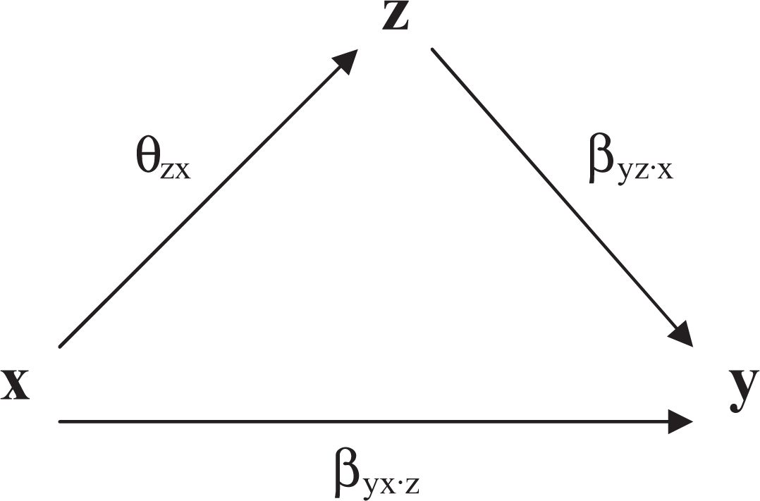
Path decomposition into direct and indirect effects.

The Binary Logit and Probit Case

The decomposition stated in equation (5) does not apply to logit and probit models. To see why this is so, we begin by deriving the logit and probit model from a latent variable model. In this case, $y^{*}$ is a continuous latent variable representing the propensity of occurrence of some outcome (e.g., propensity to complete college), x is a predictor variable of interest (e.g., parental income), and z a control variable (e.g., respondent’s academic ability). The latent variable may be thought of as a hypothetical construct, but it may also represent a real underlying variable that we have been unable to observe fully, as when we only know whether someone’s income exceeds a given value. In what follows, we once again center all variables on their respective means to avoid including intercepts in the following models. We define an underlying, latent linear model in which the latent propensity is a function of x and z:

y^{*} = β_{y x . z} x + β_{y z . x} z + u, w h e r e s d (u) = σ_{u},

where u is a random error term and $σ_{u}$ is the residual standard deviation. The model in equation (8) corresponds to the model in equation (2), except that $y^{*}$ is unobserved and we therefore cannot estimate $β_{y x . z}, β_{y z . x}, o r σ_{u.}$ ³ However, we do observe a dichotomized version of $y^{*}$ , namely $y$ , such that

\begin{aligned} y = 1 i f y^{*} > τ \\ y = 0 i f o t h e r w i s e, \end{aligned}

where τ is a threshold, which we set to zero.⁴ The expected outcome of this binary indicator is the probability of observing $y = 1$ , that is, $E (y = 1) = Pr (y = 1)$ . For further analysis, we now place an assumption on the error term, u, in equation (8). To derive the logit model, we assume that u follows a logistic distribution with zero mean and standard deviation $σ_{u}$ . We may then rewrite the error term such that $u = σ_{e} ω$ , where ω is a standard logistic random variable, with mean zero and variance $π^{2} / 3$ and $σ_{e}$ is a scale parameter, yielding a variance of $σ_{u}^{2} = σ_{e}^{2} π^{2} / 3$ for the error term in equation (10) (Amemiya 1975; Cramer 2003). The scale parameter allows the variance of the error to differ from that of the standard logistic distribution. We can then write the logit model corresponding to the linear model in equation (8) as

l o g i t [Pr (y^{*} > 0)] = b_{y x . z} x + b_{y z . x} z = \frac{β_{y x . z}}{σ_{e}} x + \frac{β_{y z . x}}{σ_{e}} z .

Equation (10) makes it clear that the logit coefficients (the b’s) are equal to the coefficients from the underlying linear model in equation (8) divided by the scale parameter of that same model:

b_{y x . z} = \frac{β_{y x . z}}{σ_{e}}; b_{y z . x} = \frac{β_{y z . x}}{σ_{e}} .

In other words, in logit models we cannot identify the underlying regression coefficient, or the scale parameter, which is a function of the residual standard deviation, but only their ratio.

To derive the probit model, assume that u follows a normal distribution with zero mean and standard deviation $σ_{u}$ . We can rewrite u as $u = σ_{e} ω$ , where ω now is a standard normal random variable, with mean zero and variance 1 and $σ_{e}$ is a scale parameter, yielding a variance of $σ_{u}^{2} = σ_{e}^{2}$ for the error term in equation (10). The probit model is given by:

Pr (y^{*} > 0) = Φ (b_{y x . z} x + b_{y z . x} z) = Φ (\frac{β_{y x . z}}{σ_{e}} x + \frac{β_{y z . x}}{σ_{e}} z) .

As in the logit case, we can identify the underlying regression coefficient only up to scale.

The coefficients in equations (11) and (12) also make it clear why we cannot compare the coefficient of x from a logit or probit model excluding the mediator z with the corresponding coefficient from a logit model including z. To see this, we specify the following reduced logit model including only x ⁵:

l o g i t (P r (y = 1)) = b_{y x} x = \frac{β_{y x} x}{{\tilde{σ}}_{e}},

which reflects the underlying linear model:

y^{*} = β_{y x} x + t,

where $t = {\tilde{σ}}_{e} υ$ . The cross-model coefficient comparison in logit models is hampered by the difference in scale parameters between equations (10) and (13).

b_{y x} - b_{y x . z} = \frac{β_{y x}}{{\tilde{σ}}_{e}} - \frac{β_{y x . z}}{σ_{e}} \neq β_{y x} - β_{y x . z} .

The relation between the scale parameters is ${\tilde{σ}}_{e} \geq σ_{e}$ , because, whenever z has an effect on y (i.e., $b_{y z \cdot x} \neq 0$ ), a model without z will have a larger residual standard deviation than a model with z because the latter model will explain more variation in the latent outcome. Thus, including a z orthogonal to x—ensuring that the y–x relationship is not mediated or confounded by z—would change the coefficient of x simply as a consequence of rescaling, as noted by Winship and Mare (1984), Yatchew and Griliches (1985), and Wooldridge (2002). In other words, the equalities stated in equation (5) for linear models do not hold for logit or probit models.

However, there exists an additional, somewhat overlooked, reason for why the equalities in equations (5) do not always hold for logit models or nonlinear probability models in general. In so far as the error, u, in equation (8) is assumed to follow a logistic distribution, it is impossible that the error in model (14), including only x, is logistically distributed. Its error will be a mixture of the logistic (u) and the distribution of z, since z is absorbed in the error term, t (Cramer 2007; Karlson et al. 2012). Thus, the logit model in equation (14) is misspecified, because the error in this reduced model is not logistic. The same results apply to the probit. More generally, we can rarely ascertain which, if any, of the models are misspecified, but the model-specific fit of the latent error to the assumed logistic or normal distribution is very likely to differ between models with different covariates. Comparing coefficients across logit or probit models without and with z will consequently not only reflect confounding and rescaling but also changes in the fit of the error to the assumed functional form.

To obtain a decomposition of total effects into direct and indirect effects, we need an approach that holds constant not only the scale but also the fit of the error to the assumed logistic or normal distribution. A solution to these issues is developed in Karlson et al. (2012). However, as we will see, an equivalent solution is to apply the “product of coefficients” method to the logit or probit model. To do so, we use the auxiliary linear regression of z on x stated in model (4), to yield the expectation:

E (z) = θ_{z x} x .

Now substitute the expression in equation (15) into the logit model in equation (10) and rearrange:

l o g i t [Pr (y^{*} > 0)] = \frac{β_{y x . z} + β_{y z . x} θ_{z x}}{σ_{e}} x .

Notice that the coefficient of x in this equation differs from that in equation (13), because of the differences in scales, ${\tilde{σ}}_{e} \geq σ_{e}$ , and because of differences in the fit to the assumed logistic distribution. This result also applies to the probit model.

However, the model in equation (16) reveals a simple decomposition of the total effect into its direct and indirect parts measured on the same scale, and the decomposition is formed using the “product of coefficients” method rather than the “difference in coefficients” method:

D i r e c t : b_{y x . z} = \frac{β_{y x \cdot z}}{σ_{e}} .

17a

{I n d i r e c t : θ}_{z x} b_{y z . x} = \frac{θ_{z x} \times β_{y z \cdot x}}{σ_{e}} .

17b

T o t a l : \frac{β_{y x}}{σ_{e}} = \frac{β_{y x \cdot z} + θ_{z x} \times β_{y z \cdot x}}{σ_{e}} .

17c

The decomposition in equation (17) is identical to the “difference in coefficients” method recently suggested by Karlson et al. (2012).⁶ It holds constant the scale and the fit of the error to the assumed distribution, because it is based on a single logit or probit model for the binary outcome, that is, the model in equation (10) or (12), and it consequently presents a generalization of the equalities in equation (5) to nonlinear probability models such as the logit or probit.

To see the equivalence between the approaches, we briefly explain the approach in Karlson et al. (2012). To make coefficients comparable across logit or probit models with different covariates, they used the following reparametrization of the model in equation (10):

l o g i t (P r (y = 1)) = b_{y x . \tilde{z}} x + b_{y \tilde{z} . x} \tilde{z} .

Here, $\tilde{z}$ is the residualized z, that is, the residual from the model in equation (4) or (15), and so $\tilde{z}$ is orthogonal to x by construction. Karlson et al. (2012) prove that

b_{y x . \tilde{z}} = \frac{β_{y x}}{σ_{e}},

and it follows that the total effect decomposes as in equation (17):

\frac{β_{y x}}{σ_{e}} = \frac{β_{y x . z} + β_{y z . x} θ_{z x}}{σ_{e}} .

The total effect and its components are measured on the scale defined by the model in equation (10) or (12), depending on whether one uses a logit or probit model. Drawing on Clogg, Petkova, and Haritou (1995), Karlson et al. (2012) name this model the “true” model, that is, the model on which inferences are based.

Although we can only point identify the total, direct, and indirect effects in logit models relative to a scale, researchers often want to assess the relative magnitude of the direct and indirect effects relative to the total effect. For this kind of decomposition, we suggest the following percentage decomposition:

\frac{b_{y z . x} \times θ_{z x}}{b_{y x . z} + b_{y z . x} \times θ_{z x}} \times 100 = \frac{\frac{β_{y z . x} \times θ_{z x}}{σ_{e}}}{\frac{β_{y x . z} + β_{y z . x} \times θ_{z x}}{σ_{e}}} \times 100 = \frac{β_{y z . x} \times θ_{z x}}{β_{y x . z} + β_{y z . x} \times θ_{z x}} \times 100,

which expresses the extent to which the x − y* relationship in a logit model is mediated, confounded, or “explained” by z. Because the direct and indirect effects sum to the total effect, it holds that the part not mediated by z, that is, the direct part, is defined as: Direct = 100 percent − Indirect. Notice also that equation (21) does not involve a scale parameter, and therefore expresses the relationship between the coefficients from the underlying linear models: in other words, it is a scale-free measure. We refer to Karlson et al. (2012) for other measures that assess the relative contributions of direct and indirect effects.

Multiple Mediators

We have provided a simple decomposition of a total logit coefficient into its direct and indirect parts and provided a simple percentage measure with which researchers may assess the relative magnitude of direct and indirect effects. Thus far, however, we have considered only one mediating variable, but in some instances we may want to consider several indirect paths by which x affects y. Because the method developed by Karlson et al. (2012) extends almost all decomposition features of linear models to logit and probit models, it is straightforward to replace a single z with a vector of mediators, z_j , where j = 1, 2, … , J, and where J denotes the total number of variables in z_j . Now we may define an underlying linear model including z_j as

y^{*} = β_{y x . z 1, . . . z J} x + \sum_{j} β_{y z (j) . x} z_{j} + t, w i t h s d (t) = σ_{t} {a n d σ}_{t}^{} = σ_{k}^{} \cdot (π^{} / \sqrt{3}) .

22a

And the corresponding logit as

l o g i t (P r (y = 1)) = b_{y x . z 1, . . ., z J} x + \sum_{j} b_{y z (j) . z} z_{j} = \frac{β_{y x . z 1, . . ., z J}}{σ_{k}} x + \sum_{j} \frac{β_{y z (j) . x}}{σ_{k}} z_{j} .

22b

Similar to equation (4), we estimate J linear regression models

z_{j} = θ_{z (j) x} + w_{j},

which provide us with J coefficients of the effect of x on each mediator. The jth indirect effect is given by

I n d i r e c t : b_{y z (j) . x} \times θ_{z (j) x} = \frac{β_{y z (j) . x} \times θ_{z (j) x}}{σ_{k}} .

24a

We refer to the sum of indirect effects over the J control variables as the grand indirect effect: $\sum_{j} b_{y z_{j} . x} θ_{z_{j} x} = \sum_{j} \frac{β_{y z (j) . x} \times θ_{z (j) x}}{σ_{k}}$ . The direct effect is given by

D i r e c t : b_{y x . z 1, . . ., z J} = \frac{β_{y x . z 1, . . ., z J}}{σ_{k}},

24b

and the total effect by

\begin{aligned} T o t a l : b_{y x . z 1, . . ., z J} + \sum_{j} b_{y z_{j} . x} θ_{z_{j} x} & = \frac{β_{y x . z 1, . . ., z J}}{σ_{k}} + \sum_{j} \frac{β_{y z (j) . x} \times θ_{z (j) x}}{σ_{k}} \\ = b_{y x . \tilde{z} 1, . . ., \tilde{z} J} \end{aligned} .

24c

That $b_{y x . \tilde{z} 1, . . ., \tilde{z} J} = \frac{β_{y x . \tilde{z} 1, . . ., \tilde{z} J}}{σ_{k}}$ follows by analogy with equation (16), and the full proof can be found in Karlson et al. (2012). The decomposition presented in equation (24) can also be used for percentage decompositions. Applying the rules in equation (21), the expressions in equation (24) can be used for quantifying the relative contribution of each control variable to both the grand indirect effect and the total effect. This follows because of the simple additivity of direct and indirect effects. The jth control variable’s contribution to the grand indirect effect is given by $\frac{b_{y z (j) . x} \times θ_{z (j) x}}{\sum_{j} b_{y z_{j} . x} θ_{z_{j} x}} \times 100$ , and its contribution to the total effect is given by $\frac{b_{y z (j) . x} \times θ_{z (j) x}}{b_{y x . z 1, . . ., z J} + \sum_{j} b_{y z_{j} . x} θ_{z_{j} x}} \times 100$ .

Holding Other Covariates Constant

In some situations, researchers will be interested in controlling the decomposition of the x − y* relationship for covariates, which represent common causes of x, z, and y. These are variables that confound the decomposition, that is, the estimates of both direct and indirect effects. Let w_i denote the ith confounding covariate, i = 1, 2, … , I. We can control for the potential confounding influence of these covariates on the decomposition by including w_i as covariates in each of the equations defining the system of interest. Assume, for simplicity, that we have a single control variable, z. We define an underlying linear model as

\begin{aligned} y^{*} & = β_{y x . z, w_{1} . . . w_{I}} x + β_{y z . x, w_{1} . . . w_{I}} z + \sum_{i} β_{y w_{i} . x, z} w_{i} + s, w i t h s d (s) \\ = σ_{s} {a n d σ}_{s}^{} = σ_{l}^{} \times (π^{} / \sqrt{3}), \end{aligned}

25a

and the corresponding logit model

\begin{aligned} l o g i t (Pr (y = 1)) & = b_{y x . z, w_{1} . . . w_{I}} x + b_{y z . x, w_{1} . . . w_{I}} z + b_{y w_{i} . x, z} w \\ = \frac{β_{y x . z, w_{1} . . . w_{I}}}{σ_{l}} x + \frac{β_{y z . x, w_{1} . . . w_{I}}}{σ_{l}} z + \sum_{i} \frac{β_{y w_{i} . x, z}}{σ_{l}} w_{i}, \end{aligned}

25b

where $σ_{l} \leq σ_{e}$ , because the added covariates, insofar they explain variation in the latent propensity, reduce the residual variation. We also define an equation similar to that in equation (4), except that the covariates now enter the equation:

z = θ_{z x . w_{1} . . . w_{I}} x + \sum_{i} θ_{z w_{i} . x} w_{i} + q,

25c

with q being the error term. Using the three equations in equation (25), we may decompose the total effect net of possibly confounding covariates into its direct and indirect parts.

Binary Mediators

Up to this point, we have assumed that the mediating variable, z, is continuous (notice that x could have been continuous or dichotomous). What happens to the decomposition when the observed mediating variable is binary? In the linear case, where y* is continuous, we have:

y^{*} = γ_{y x . z^{*}} x + γ_{y z^{*} . x} z^{*} + σ_{n} ω,

26a

where z* is the dichotomous mediating variable and the error term is rewritten as previously explained. In general, $γ_{y x . z^{*}} \neq β_{y x . z}$ and $γ_{y z^{*} . x} \neq β_{y z . x}$ . Nevertheless, given the linear probability model

z^{*} = φ_{z^{*} x} x + m,

26b

where m is an error term, it remains the case that

β_{y x} = γ_{y x . z^{*}} + φ_{z^{*} x} γ_{y z^{*} . x} .

26c

That is to say, the total effect of x on y decomposes into a direct and indirect effect, given that the effect of x on z* is estimated using a linear probability model and not a logit or other nonlinear probability model.

Given y, a binary realization of y*, we estimate the logit:

l o g i t (Pr (y = 1)) = c_{y x . z} x + c_{y z^{*} . x} z^{*} = \frac{γ_{y x . z^{*}} x + γ_{y z^{*} . x} z^{*}}{σ_{n}} .

Then the decomposition of the total effect into direct and indirect components is:

\frac{γ_{y x}}{σ_{n}} = c_{y x . {\tilde{z}}^{*}} = \frac{γ_{y x . z^{*}} + φ_{z^{*} x} γ_{y z^{*} . x}}{σ_{n}},

where $c_{y x . {\tilde{z}}^{*}}$ is the logit coefficient for x in the model which controls for the residualized z*.

Reporting Average Partial Effects

The method we have presented can also be applied to average partial effects (APEs: Wooldridge 2002:22-4). One advantage of APEs over logit or probit coefficients is that they are measured on the probability scale and are therefore intuitive and more easily understood than, say, partial log odds ratios.

In logit models, the marginal effect (ME), of x is the derivative of the predicted probability with respect to x, given by (when x is continuous and differentiable):

\frac{d \hat{p}}{d x} = \hat{p} (1 - \hat{p}) b = \hat{p} (1 - \hat{p}) \frac{β}{σ} = \frac{\hat{p} (1 - \hat{p})}{σ} β,

where $\hat{p} = Pr (y = 1 | x)$ is the predicted probability, given x and $b = \frac{β}{σ}$ is the logit coefficient of x. The APE is the average value of this derivative over the whole population:

\frac{1}{N} \sum_{i = 1}^{N} \frac{d {\hat{p}}_{i}}{d x_{i}} = \frac{1}{N} \sum_{i = 1}^{N} \frac{{\hat{p}}_{i} (1 - {\hat{p}}_{i})}{σ} β .

If the sample is drawn randomly from the population, then the APE estimates the average ME of x in the population. Let p denote the probability of y = 1 for the model with both x and z (or $\tilde{z}$ ) included as predictors. We then have (omitting the i subscript for convenience):

\begin{aligned} p = Pr (Y = 1 | x, z) = F (\frac{β_{y x . z} x + β_{y z . x} z}{σ}) \\ = Pr (y = 1 | x, \tilde{z}) = F (\frac{(β_{y x . z} + β_{y z . x} θ_{z x}) x + β_{y \tilde{z} . x} \tilde{z}}{σ}), \end{aligned}

where $F (x) = exp (x) / (1 + exp (x))$ is the logistic distribution function and where θ is, as previously, the coefficient from the linear regression of z on x; β is the partial underlying regression coefficient, controlling for z, of y on x; and σ is the scale parameter. We can now easily find the direct effect as $\sum_{i = 1}^{N} \partial F (\frac{β_{y x . z} x + β_{y z . x} z}{σ}) / \partial x$ . The indirect effect is given by $\sum_{i = 1}^{N} \partial F \frac{[\frac{β_{y x . z} x + β_{y z . x} z}{σ}]}{\partial z} \frac{\partial z}{\partial x}$ . The total effect is the sum of these two. Similar to equation (17), the direct, indirect, and total effects are given by:

D i r e c t : A P E (b_{y x . z}) = \frac{1}{N} \sum_{i = 1}^{N} \frac{p (1 - p)}{σ} β_{y x . z}

31a

I n d i r e c t : A P E (b_{y z . x}) \times θ_{z x} = \frac{1}{N} \sum_{i = 1}^{N} \frac{p (1 - p)}{σ} β_{y z . x} θ_{z x}

31b

T o t a l : A P E (b_{y x . z}) + A P E (b_{y z . x}) \times θ_{z x} = \frac{1}{N} \sum_{i = 1}^{N} \frac{p (1 - p)}{σ_{}} (β_{y x . z} + β_{y z . x} θ_{z x}) .

31c

The total effect measured in APEs corresponds to the total effect, $b_{y x . \tilde{z}}$ , as this is defined in equation (18) (see Karlson et al. 2012). These results extend easily to the probit case, in which we replace the expression of the partial effect with the partial derivative $\frac{d \hat{p}}{d x} = \frac{φ (\hat{p})}{σ} β$ , where $φ (.)$ is the standard normal p.d.f.

Conditions for Causal Mediation Analysis

In recent years, methodologists have criticized mediation analysis for lacking a causal interpretation (e.g., Jo 2008; Pearl 2001; Robins and Greenland 1992; Sobel 2008). Subsequent work by Imai, Keele, and Tingley (2010) and Imai, Keele, and Yamamoto (2010) have clarified the conditions under which mediation effects can be given a causal interpretation: Under the sequential ignorability assumption, SIA, mediation effects are nonparametrically identified. The SIA consists of two assumptions (Imai, Keele, and Tingley 2010; Imai, Keele, and Yamamoto 2010)⁷:

Predictor variable x is conditionally independent of unobservables, u, given background covariates w: $x ⊥ u | w$ .

Mediator variable z is conditionally independent of unobservables, u, given background covariates w and predictor variable x: $z ⊥ u | x, w$ .

As noted by Imai, Keele, and Tingley (2010), a randomized experiment automatically ensures that assumption 1 holds, but not that assumption 2 holds, because individuals can still self-select into the mediator, z (Sobel 2008).⁸ In observational studies, we assume that conditioning on covariates w controls for the selection on unobservables that, in absence of controlling, would render the mediation analysis biased.

Imai, Keele, and Yamamoto (2010) prove that under SIA, mediation effects can be given a causal interpretation. They show that this result holds for mediation analysis in linear models and they present, among others, a method for estimating mediation analysis in nonlinear probability models. Before we turn to a comparison of our method with theirs, we notice that, given the identification results in Imai, Keele, and Yamamoto (2010), under SIA, our method also identifies causal mediation effects. And the effects identified by our model are measured on the scale of the “true” model because the method we suggest applies to the coefficients of the underlying linear models, and so, given the applicability of the identification result to linear models, our method also identifies causal mediation effects under the SIA.

Comparing the Two Approaches Using Monte Carlo Simulations

Imai, Keele, and Tingley (2010) and Imai, Keele, and Yamamoto (2010) develop their own method for estimating mediation effects in nonlinear probability models such as the logit or probit. To briefly explain the approach, assume that y and x (the treatment variable) are both binary, z is continuous, and the SIA is met without controlling for covariates w. The approach is very similar to the one we suggest here, but differs in that it approximates the distributions of interest with a quasi-Bayesian Monte Carlo algorithm, using the predictions of models for the mediator and for the outcome. This means that for nonlinear probability models such as the logit or probit, the approach of Imai et al. reports effects on the probability scale, not on the logit or probit scale. This property of the method also means that, whenever outcomes are ordinal or multinomial, the method produces several mediation effects on the probability margin. In the context of binary parametric nonlinear probability models, the algorithm for estimating causal mediation effects is (Imai, Keele, and Tingley 2010a:317):

Estimate a logit or probit model of y on x and z, and a linear model of z on x.

Simulate parameters of each model from their sampling distribution.

Simulate the potential values of the mediator, simulate the potential outcomes given the simulated values of the mediator, and compute the causal mediation effects.

Compute summary statistics from the simulations.

To compare the performance of our method relative to that of Imai and colleagues, we ran a Monte Carlo simulation based on the following model:

\begin{aligned} y^{*} = β x + γ z + e \\ z = θ x + u, \\ y = 1 i f y^{*} > q, y = 0 o t h e r w i s e, \end{aligned}

where x is a binary variable distributed 30/70, 50/50, or 70/30 in three different simulations, respectively, z is a continuous variable, e is drawn from a logistic (correctly specified error, because we fit a logit model) or normal (incorrectly specified) distribution, standardized to mean zero and $π^{2} / 3$ variance, u is drawn from a normal or lognormal distribution standardized to mean zero and unit variance. In all models, $s d (x) = s d (z) = 1$ , and consequently $ρ (x, z) = {0.0, 0.3, 0.6, 0.9}$ , where $ρ (x, z)$ is the correlation coefficient between x and z. The threshold, q, is chosen such that y takes on the following distributions: 50/50, 75/25, 95/5. This setup produces four (A, B, C, D) times two different scenarios (correctly and misspecified error term) in which $θ = ρ (x, z)$ and q varies. In the first four scenarios, e is logistically distributed and the model is consequently correctly specified. In the second four scenarios, e is normally distributed and the model is consequently misspecified. Scenarios A, B, C, and D differ according to the following specifications:

A: $β = 1$ and $γ = 0.5$ , and z is a mixture of a binary and a normal variable.

B: $β = 1$ and $γ = 0.5$ , and z is a mixture of a binary and a lognormal variable.

C: $β = 0.5$ and $γ = 1$ , and z is a mixture of a binary and a normal variable.

D: $β = 0.5$ and $γ = 1$ , and z is a mixture of a binary and a lognormal variable.

We measure performance in terms of the accuracy with which each method estimates the mediation percentage; that is, the ratio of the indirect to the total effect. We used the logit model in all simulations, and based our study on 500 repetitions using N = 5,000. The full output of the simulation study is reported in the Appendix which can be found at http://smr.sagepub.com/supplemental/.

In Table 1, we report the average absolute difference between the estimated and the true mediation percentage in each of the four scenarios with correctly specified and misspecified errors. We find that, across all scenarios, our method (labeled KHB) and the method of Imai et al. return near-identical results and both are almost as good as the (estimated) latent linear model in recovering the true mediation percentage. However, even though the two methods perform equally well in terms of recovering the true mediation percentage, our method has three comparative advantages: (1) It is computationally simpler; (2) it allows for effects measured on both the logit or probit scale and the probability scale; and (3) because our method concerns the underlying parameters generating the data, it easily extends to the case with ordered outcome variables.

Table 1.

Summary of Monte Carlo Simulations. Mean Absolute Difference to the True Mediation Percentage Times 1,000 Reported.

	1: Logistic Error (Correctly Specified)			2: Normal Error (Misspecified)
	Latent Linear	KHB	Imai et al.	Latent Linear	KHB	Imai et al.
A	1.98	2.09	2.06	1.29	2.08	2.21
B	0.09	0.89	1.16	0.24	1.33	0.94
C	2.76	3.46	3.48	2.04	3.04	3.00
D	0.28	1.20	1.21	0.70	1.88	1.84
M	1.28	1.91	1.98	1.07	2.08	2.00

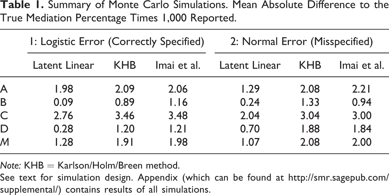
Note: KHB = Karlson/Holm/Breen method.

See text for simulation design. Appendix (which can be found at http://smr.sagepub.com/supplemental/) contains results of all simulations.

Alternative Solutions

Using Monte Carlo simulations, Karlson et al. (2012) compared the method we propose with other methods for comparing coefficients across same-sample nested logit or probit models. They found that, for estimating mediation effects, their method is always as good as or better than the linear probability model, APEs based on the logit or probit (Cramer 2007; Wooldridge 2002), and the method of Y standardization (Long 1997; Winship and Mare 1984). In particular, the linear probability model and the method of Y standardization return biased estimates of mediation effects in certain situations met in real applications (Best and Wolf 2012). The method of Y standardization was particularly sensitive to changes in the distribution of the error across models caused by successively adding covariates, because this changes the fit of the model to the assumed logistic or normal distribution. Indeed, all three alternative methods discussed in Karlson et al. (2012) are based on estimating different models, thereby reflecting changes in the fit of the error to the assumed distribution. But the method we propose effectively overcomes this issue, because it holds constant the model on which we want to base our inferences.

Interaction Term between the Predictor and the Mediator

Researchers are sometimes interested in testing whether mediation effects differ between groups. Such group comparisons are straightforward to examine using the method presented in this article. In these cases, researchers can apply the Karlson/Holm/Breen (KHB) method to each group separately and compare the scale-free percentage decomposition. However, a special case arises when the predictor variable and the mediator variable are interacted (Kraemer et al. 2008). Using the rules of differential calculus, Stolzenberg (1980) gave the derivations for the linear model. He found that, in this case, the indirect effect depends on the level of the predictor variable, thereby introducing heterogeneity into the indirect effects. In the approach by Imai, Keele, and Tingley (2010) and Imai, Keele, and Yamamoto (2010), this heterogeneity is translated into mediation effects for the treated (x = 1) and the untreated (x = 0) in situations where x is a binary dummy.

However, while these results are straightforward to derive in the linear setting, in nonlinear probability models such as the logit or probit, the difference in the indirect effects for the treated and untreated is possibly confounded by differences in scales across the groups defined in x; that is, by heteroscedasticity in the latent errors. To see this, assume that the underlying linear model is heteroscedastic across the two groups in x = 0,1:

\begin{aligned} y_{}^{*} = α + β_{y z . x} z + σ_{0} ω i f x = 0 \\ y_{}^{*} = (α + β_{y x . z}) + (β_{y z . x} + δ_{y z . x}) z + σ_{1} ω i f x = 1, \end{aligned}

where α is a constant term, $β_{y z . x}$ is the effect of x on y*, and $δ_{y z . x}$ is the interaction effect of x and z on y* and $σ_{j}, j = 0, 1$ are scale factors in the two groups (x = 0, 1). If we derive the logit or probit including an interaction term between x and z from the underlying model in equation (32), we obtain the following indirect effects for the treated and untreated:

x = 0 : \frac{β_{y z . x} θ_{z x}}{σ_{0}} .

33a

x = 1 : \frac{(β_{y z . x} + δ_{y z . x}) θ_{z x}}{σ_{1}} .

33b

These indirect effects differ not only in terms of the coefficients of interest in the numerators (i.e., their location), $β_{y z . x} θ_{z x}$ and $(β_{y z . x} + δ_{y z . x}) θ_{z x}$ , but also in their scales, $σ_{0}$ and $σ_{1}$ . Because we cannot know the relation between the scales (Allison 1999), we cannot compare the indirect effects across untreated and treated. In other words, comparisons of the indirect effects of interest are confounded by latent error heteroscedasticity.⁹

The result in equation (33) shows that using interaction terms between the predictor and the mediator in nonlinear probability models identifies indirect effects for the treated and untreated, but up to scales whose relation is unknown. Differences in these effects can consequently result from differences in true indirect effects, in scale parameters, or in both. Under the assumption that scales do not differ, we can meaningfully compare indirect effects, but this assumption cannot be tested without credible exclusion restrictions. We therefore suggest that social researchers exercise caution in inferring heterogeneity in mediation effects across treated and untreated—or more generally across levels in the predictor variable—in nonlinear probability models.

Examples

In this section, we turn to two examples based on the National Educational Longitudinal Survey of 1988 (NELS). NELS is a nationally representative survey of eighth grade students in the United States in 1988 who were followed until the year 2000, giving us the opportunity to study educational progress. We examine how much of the effect of parental socioeconomic status (SES) on four-year college graduation (COL) by year 2000 is mediated by student academic ability (ABIL) and level of educational aspiration (LEA).¹⁰ We standardize SES, ABIL, and LEA to have mean zero and variance of unity. Because we expect ability and aspirations to be positively correlated with parental SES and college graduation (e.g., Boudon 1974; Keller and Zavalloni 1964), we expect that both ability and aspirations mediate the effect of parental SES on college graduation. We also investigate whether ability or aspirations is the larger mediator. Because we suspect the decomposition to be affected by potentially confounding variables, we also include covariates, gender (MALE), race (RACE), and intact family (INTACT). The final sample comprises 9,820 individuals, and Table 2 contains the descriptive statistics.¹¹ We calculate the decompositions using the Stata command khb (Kohler, Karlson, and Holm 2011), which implements the method developed by Karlson et al. (2012) and the innovations presented in this article.

Table 2.

Variable Descriptive.

	Mean	SD
COL	0.36	—
SES	0	1
ABIL	0	1
LEA	0	1
MALE	0.47	—
RACE
White (reference)	0.69	—
Hispanic	0.12	—
Black	0.09	—
Other	0.10	—
INTACT	0.90	—

Note: N = 9,820. ABIL = student academic ability; COL = college graduation; SES = socioeconomic status; LEA = level of educational aspiration.

We structure the analysis in four steps. First, we decompose the effect of SES on COL using ABIL. Second, we add LEA to the decomposition and evaluate which variable, ABIL or LEA, has the larger indirect effect. Third, we add three covariates, MALE, RACE, and INTACT to the decomposition to control for possibly confounding variables. Fourth, we report the results in terms of APEs, giving the decomposition a more substantive interpretation. Because the results may be sensitive to model choice, we report them for both logit and probit models.

Table 3 reports the results of a decomposition of SES on COL with ABIL as the mediator. Using the expressions in 17a to c (decomposition using the “product of coefficients” method), we decompose, in logits (probits) the total effect of 1.348 (0.781) into a direct part, 0.914 (0.524), and an indirect part, 0.434 (0.257). Using the test statistic developed in Karlson et al. (2012), we see that all effects are highly statistically significant. We also see that the indirect effect is around half the magnitude of the direct effect. In relative terms, the indirect effects accounts for 32.2 percent of the total effect in the logit model and 32.9 percent in the probit model. In the second row from the bottom of Table 3, we label this the mediation percentage. This is very similar for the logit and probit, indicating that our decomposition is not sensitive to the choice of a normal or logistic error distribution for the full model including both SES and ABIL. In the final row, we report the naive mediation percentage, which is what we would have obtained had we simply compared the coefficients across models with and without ABIL. This is 25.3 percent for the logit model and 26.8 percent for the probit model, indicating that a naive comparison of effects would underestimate the true amount of mediation net of rescaling and changes in the error to the assumed distribution.

Table 3.

Decomposition of Total Effect of SES on COL into Direct Effect and Indirect Effect via ABIL.

	Logit		Probit
	Coefficient	z	Coefficient	Z
Coefficients
Total effect	1.348	42.06	0.781	45.23
Direct effect	0.914	28.90	0.524	29.57
Indirect effect	0.434	26.06	0.257	26.79
Relative measures
Mediation percentage	32.2	—	32.9	—
Naive mediation percentage	25.3		26.8

Note: COL = college graduation; ABIL = student academic ability; SES = socioeconomic status.

In Table 4, we add LEA to the decomposition and break down the indirect effect due to both ABIL and LEA into its respective components. We see that all effects are highly statistically significant. Because the logit and probit return near-identical results, we focus only on the results based on the former. Looking at the relative measures of the indirect effect, we see that, compared to Table 3, the mediation percentage has increased from 32.2 to 56.6 percent. However, more of the effect of SES is mediated by LEA than by ABIL, LEA accounting for 37.5 percent of the total effect, ABIL for 19.1 percent. The mediation percentage for ABIL is considerably smaller than the 32.2 percent reported in Table 3. Thus, including LEA in the decomposition reduces the contribution of ABIL to the total effect by about 13 percentage points, and this is because LEA is positively correlated with SES, ABIL, and COL. We also see that the naive use of the logit would underestimate the mediation percentage by about 15 percentage points (41.3 percent compared with 56.6 percent).

Table 4.

Decomposition of Total Effect of SES on COL Into Direct Effect and Indirect Effect via ABIL and LEA.

	Logit		Probit
	Coefficient	Z	Coefficient	Z
Coefficients
Total effect	1.657	42.83	0.939	46.33
Direct effect	0.718	21.48	0.421	22.31
Indirect effect	0.938	29.80	0.518	30.67
via ABIL	0.317	18.87	0.192	19.78
via LEA	0.621	22.55	0.326	23.58
Relative measures
Mediation percentage	56.6	—	55.2	—
via ABIL	19.1	—	20.4	—
via LEA	37.5	—	34.7	—
Naive mediation percentage	41.3	—	41.2	—

Note: COL = college graduation; ABIL = student academic ability; LEA = level of educational aspiration; SES = socioeconomic status.

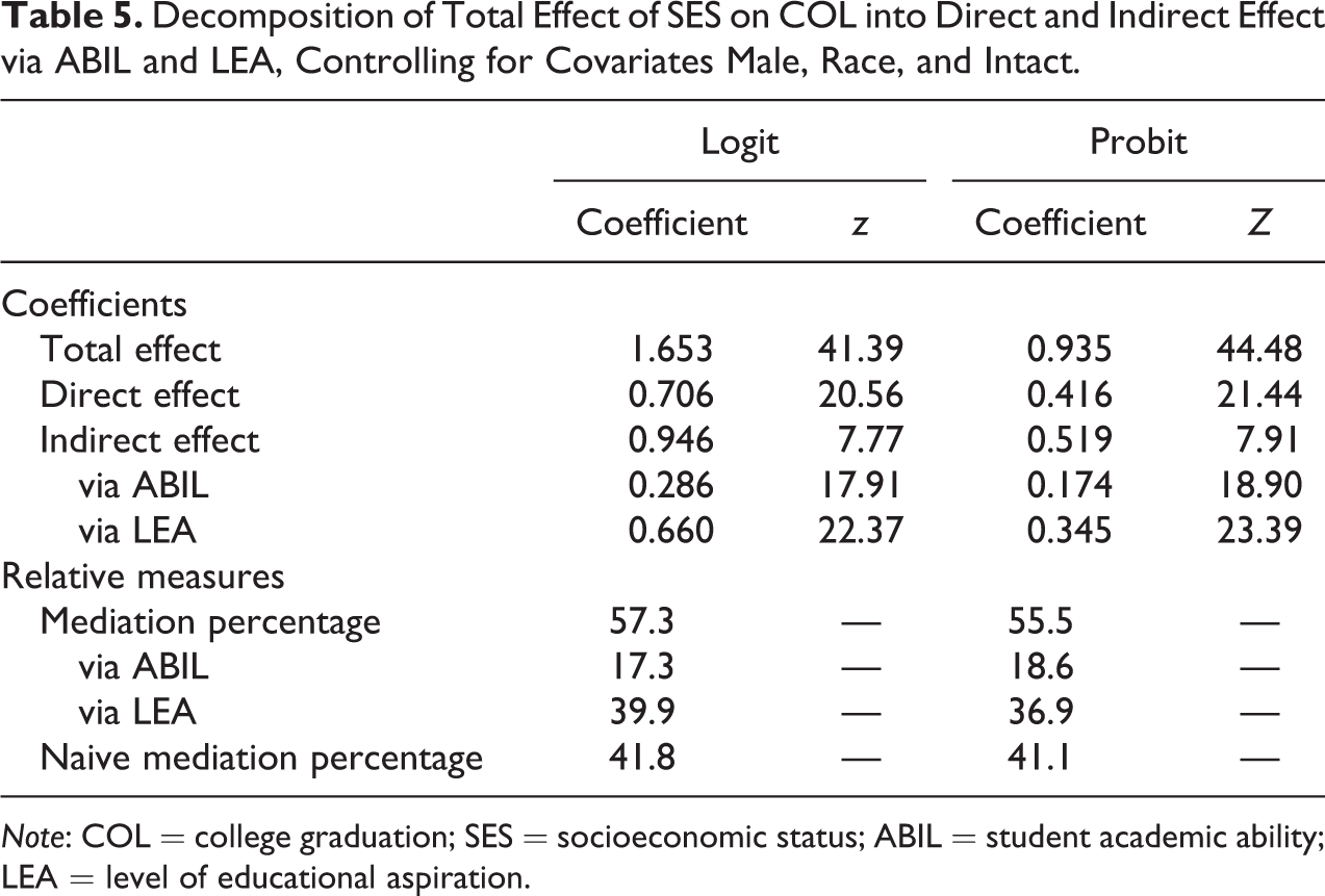
In Table 5 we add three covariates, MALE, RACE, and INTACT, which we suspect may confound the decomposition. These covariates are included in all models used for the decomposition, thereby holding constant their possible influence on the results. We see that the results are virtually identical to those reported in Table 4, except for the test statistic for the indirect effect. This statistic reduces markedly to 7.77 in the logit case. However, the effect is still highly statistically significant. Thus, these findings suggest that the substantive results presented in Table 4 are unaffected by the influence of the covariates.

In Table 6, we report APEs of the results in Table 5, using formulae 31a to c, the product of coefficients decomposition rule for APEs. Because the standard error of the indirect effect is unknown, we only report the APEs and once again we focus on the results from the logit model. We see that the total effect is 0.228, which means that for a standard deviation change in SES, the probability of graduating college increases, on average, by 22.8 percentage points. Decomposing this effect returns a direct effect of 9.7 percentage points, and an indirect of 13.0 percentage points. Breaking down the indirect effect to its two components, we find that the indirect effect via ABIL is 3.9 percentage points, and 9.1 percentage points via LEA. Thus, the effect of SES on COL running via LEA is substantially larger than the one running through ABIL. We note that the mediation percentages in Table 6 equal those in Table 5. However, the naive mediation percentage in the final column differs between the two tables. In Table 5, the naive percentage conflates mediation and rescaling, while the counterpart in Table 6 conflates mediation with the sensitivity of APEs to changes in the error distribution across models excluding and including the control variables. As we would expect, the naive mediation percentage is much smaller for the APE than for the logit. APE underestimates the true percentage by about 3 percentage points compared with the underestimate from the logit of 15 percentage points.

Table 5.

Decomposition of Total Effect of SES on COL into Direct and Indirect Effect via ABIL and LEA, Controlling for Covariates Male, Race, and Intact.

	Logit		Probit
	Coefficient	z	Coefficient	Z
Coefficients
Total effect	1.653	41.39	0.935	44.48
Direct effect	0.706	20.56	0.416	21.44
Indirect effect	0.946	7.77	0.519	7.91
via ABIL	0.286	17.91	0.174	18.90
via LEA	0.660	22.37	0.345	23.39
Relative measures
Mediation percentage	57.3	—	55.5	—
via ABIL	17.3	—	18.6	—
via LEA	39.9	—	36.9	—
Naive mediation percentage	41.8	—	41.1	—

Note: COL = college graduation; SES = socioeconomic status; ABIL = student academic ability; LEA = level of educational aspiration.

Table 6.

APE Decomposition of Total Effect of SES on COL into Direct and Indirect Effect via ABIL and LEA, Controlling for Covariates Male, Race, and Intact.

	Logit	Probit
	APE	APE
Coefficients
Total effect	0.2276	0.2233
Direct effect	0.0973	0.0994
Indirect effect	0.1303	0.1239
via ABIL	0.0394	0.0416
via LEA	0.0909	0.0823
Relative measures
Mediation percentage	57.3	55.5
via ABIL	17.3	18.6
via LEA	39.9	36.9
Naive mediation percentage	54.2	53.1

Note: APEs = average partial effects; ABIL = student academic ability; LEA = level of educational aspiration.

Conclusion

In this article, we suggest an approach for estimating and interpreting total, direct, and indirect effects in nonlinear probability models such as the logit and probit. Our method is derived from a linear latent variable model assumed to underlie the logit or probit model, and it extends the decomposition properties of linear models to nonlinear probability models. We developed several extensions of the method; in particular, we applied it to APEs, giving researchers an effect measure on the probability scale which may be more interpretable than logit and probit coefficients, and we showed that the indirect effects can be given a causal interpretation under the SIA suggested by Imai, Keele, and Tingley (2010) and Imai, Keele, and Yamamoto (2010).

A Monte Carlo study comparing the method with that of Imai, Keele, and Tingley (2010) and Imai, Keele, and Yamamoto (2010) showed that both perform equally well in recovering the true mediation percentage. The difference between the methods in terms of estimation is therefore negligible, but ours is computationally simpler, allows for effects measured on both the logit or probit index and the probability scale, and easily generalizes to the situation with ordered outcomes. Further analytical results suggested that while indirect effects for the treated and untreated can be identified in nonlinear probability models involving an interaction effect between the mediator and the predictor, they are identified up to different scales and are consequently not comparable. Thus, researchers should exercise caution in interpreting such heterogeneity in mediation effects.

Because of its generality, our method can be extended to the ordered and multinomial case and potentially to the class of generalized linear models. Perhaps most usefully, the method can be applied very easily using the Stata routine khb (Kohler et al. 2011).

Footnotes

Declaration of Conflicting Interests

The author(s) declared no potential conflicts of interest with respect to the research, authorship, and/or publication of this article.

Funding

The author(s) received no financial support for the research, authorship, and/or publication of this article.

Notes

References

Allison

Paul D

. 1999. “Comparing Logit and Probit Coefficients Across Groups.” Sociological Methods & Research 28:186–208.

Alwin

Duane

Hauser

Robert M.

. 1975. “The Decomposition of Effects in Path Analysis.” American Sociological Review 40:37–47.

Amemiya

Takeshi

. 1975. “Qualitative Response Models.” Annals of Economic and Social Measurement 4:363–88.

Best

Henning

Wolf

Christof

. 2012. “Modellvergleich und Ergebnisinterpretation in Logit- und Probit-Regressionen.” Kölner Zeitschrift für Soziologie und Sozialpsychologie 64:377–95.

Blalock

Hubert M.

1979. Social Statistics. 2nd ed. New York: McGraw-Hill.

Bollen

Kenneth A

. 1987. “Total, Direct and Indirect Effects in Structural Equation Models.” Sociological Methodology 17:37–69.

Boudon

Raymond

. 1974. Education, Opportunity and Social Inequality. New York: John Wiley.

Breen

Richard

Goldthorpe

John H.

. 1997. “Explaining Educational Differentials: Towards a Formal Rational Action Theory.” Rationality and Society 9:275–305.

Cameron

Stephen V.

Heckman

James J.

. 1998. “Life Cycle Schooling and Dynamic Selection Bias: Models and Evidence for Five Cohorts of American Males.” Journal of Political Economy 106:262–333.

10.

Clogg

Clifford C.

Petkova

Eva

Haritou

Adamantios

. 1995. “Statistical Methods for Comparing Regression Coefficients between Models.” The American Journal of Sociology 100:1261–93.

11.

Cramer

J. S

. 2003. Logit Models. From Economics and Other Fields. Cambridge, England: Cambridge University Press.

12.

Cramer

J. S

. 2007. “Robustness of Logit Analysis: Unobserved Heterogeneity and Mis-specified Disturbances.” Oxford Bulletin of Economics and Statistics 69:545–55.

13.

Duncan

Otis

. 1966. “Path Analysis: Sociological Examples.” The American Journal of Sociology 72:1–16.

14.

Erikson

Robert

Goldthorpe

John H.

Jackson

Michelle

Yaish

Meir

Cox

D. R.

. 2005. “On Class Differentials in Educational Attainment.” Proceedings of the National Academy of Science (PNAS) of the USA 102:9730–33.

15.

Fienberg

Stephen E.

1977. The Analysis of Cross-classified Categorical Data. Cambridge, MA: MIT Press.

16.

Hosmer

David W.

Lemeshow

Stanley

. 1989. Applied Logistic Regression. New York: John Wiley.

17.

Imai

Kosuke

Keele

Luke

Tingley

Dustin

. 2010. “A General Approach to Causal Mediation Analysis.” Psychological Methods 15:309–34.

18.

Imai

Kosuke

Keele

Luke

Yamamoto

Teppei

. 2010. “Identification, Inference, and Sensitivity Analysis for Causal Mediation Effects.” Statistical Science 25:51–71.

19.

Booil

. 2008. “Causal Inference in Randomized Experiments with Mediational Processes.” Psychological Methods 13:314–36.

20.

Karlson

Kristian B.

Holm

Anders

. 2011. “Decomposing Primary and Secondary Effects: A New Decomposition Method.” Research in Stratification and Social Mobility 29:221–37.

21.

Karlson

Kristian B.

Holm

Anders

Breen

Richard

. 2012. “Comparing Regression Coefficients Between Same-Sample Nested Models using Logit and Probit: A New Method.” Sociological Methodology 42:286–313.

22.

Keller

Suzanne

Zavalloni

Marisa

. 1964. “Ambition and Social Class: A Respecification.” Social Forces 43:58–70.

23.

Kohler

Ulrich

Karlson

Kristian B.

Holm

Anders

. 2011. “Comparing Coefficients of Nested Nonlinear Probability Models.” The Stata Journal 11:1–19.

24.

Kraemer

Helena C.

Kiernan

Michaela

Essex

Marilyn

Kupfer

David J.

, 2008. “How and Why Criteria Defining Moderators and Mediators Differ between the Baron and Kenny and MacArthur Approaches.” Health Psychology 27:S101–108.

25.

Long

J. S

. 1997. Regression Models for Categorical and Limited Dependent Variables. Thousand Oaks, CA: Sage.

26.

MacKinnon

David P.

Dwyer

James H.

. 1993. “Estimating Mediated Effects in Prevention Studies.” Evaluation Review 17:144–58.

27.

McKelvey

Richard D.

Zavoina

William

. 1975. “A Statistical Model for the Analysis of Ordinal Level Dependent Variables.” Journal of Mathematical Sociology 4:103–20.

28.

Morgan

Stephen L.

2012. “Models of College Entry and the Challenges of Estimating Primary and Secondary Effects.” Sociological Methods and Research 41:17–56.

29.

Pearl

Judea

. 2001. “Direct and indirect effects.” Pp. 411–20 in Proceedings of the Seventeenth Conference on Uncertainty and Artificial Intelligence, edited by Breese

John

Koller

Daphne

. San Francisco, CA: Morgan Kaufmann.

30.

Powers

Daniel A.

Xie

. 2000. Statistical Methods for Categorical Data Analysis. San Diego, CA: Academic Press.

31.

Robins

James M.

Greenland

Sander

. 1992. “Identifiability and Exchangeability for Direct and Indirect Effects.” Epidemiology 3:143–55.

32.

Rubin

Donald B.

1974. “Estimating Causal Effects of Treatments in Randomized and Nonrandomized Studies.” Journal of Educational Psychology 66:688–701.

33.

Rubin

Donald B.

1978. “Bayesian Inference for Causal Effects: The Role of Randomization.” The Annals of Statistics 6:34–58.

34.

Stolzenberg

Ross M.

1980. “The Measurement and Decomposition of Causal Effects in Nonlinear and Nonadditive Models.” Pp. 459–88 in Sociological Methodology, edited by Schuessler

. San Francisco, CA: Jossey-Bass.

35.

Sobel

Michael E

. 2008. “Identification of Causal Parameters in Randomized Studies with Mediating Variables.” Journal of Educational and Behavioral Statistics 33:230–51.

36.

Winship

Christopher

Mare

Robert D.

. 1983. “Structural Equations and Path Analysis for Discrete Data.” The American Journal of Sociology 89:54–110.

37.

Winship

Christopher

Mare

Robert D.

. 1984. “Regression Models with Ordinal Variables.” American Sociological Review 49:512–25.

38.

Wooldridge

Jeffrey M.

2002. Econometric Analysis of Cross Section and Panel Data. Cambridge, MA: MIT Press.

39.

Yatchew

Adonis

Griliches

Zvi

. 1985. “Specification Error in Probit Models.” The Review of Economics and Statistics 67:134–39.