
Abstract
The dissimilarity index of Duncan and Duncan is widely used in a broad range of contexts to assess the overall extent of segregation in the allocation of two groups in two or more units. Its sensitivity to random allocation implies an upward bias with respect to the unknown amount of systematic segregation. In this article, following a multinomial framework based on the assumption that individuals allocate themselves independently and that unit sizes are not fixed, we provide (1) a mathematical proof of the nonnegativity of the bias, (2) an analytic way of obtaining the same results of a recent bootstrap-based bias correction but without using resampling, and (3) a new bias correction that outperforms, in terms of both bias and mean square error, those based on grouped jackknife, bootstrap, and double bootstrap.
Introduction
The study of segregation of demographic groups, often related to ethnicity or gender, is a major topic of research for economists, demographers, and other social scientists. In almost all applications, the assessment of the amount of segregation within a community is based on the proportions of demographic groups afferent to some kind of allocation units, such as residential areas, workplaces, or schools.
Many segregation indexes have been suggested, with different formulations referring to different definitions of segregation (for an overview, see Massey and Denton 1988; White 1986). Among these, the dissimilarity index D, proposed by Duncan and Duncan (1955), is widely used to assess the differential distribution of two groups among allocation units. This index has been used in a broad range of contexts, such as gender segregation (see, e.g., Deutsch and Silber 2005; Kakwani 1994; Karmel and Maclachlan 1988), labor force segregation (for a survey, see Flückiger and Silber 1999; also see Silber 1989, where D is compared to alternative indexes of segregation, Carrington and Troske 1997, and Silber, Flückiger, and Reardon 2009), and residential segregation (see Duncan and Duncan 1955; Farley 1975; Taeuber and Taeuber 1965, who also faces school segregation, and Massey and Denton 1987, 1988).
The observed allocation pattern is one of the possible outcomes of a random process that is characterized by a certain level of “systematic” segregation, the resulting of a mix of behavior-based forces. In this view, the observed dissimilarity
Within a multinomial framework based on the assumption that individuals allocate themselves independently and that unit sizes are not fixed (see the second section), Allen, Burgess, and Windmeijer (2009) demonstrate, using simulations, that random allocation generates substantial unevenness, and hence an upward bias, especially when dealing with small units, a small minority proportion, and a low level of segregation. Other authors, using different frameworks, arrive at the same conclusions (see, e.g., Carrington and Troske 1997; Cortese, Falk, and Cohen 1976; Farley and Johnson 1985; Ransom 2000). In the third section, we first outline, using simulations, the effect of some relevant factors to the bias magnitude and then we provide an analytical proof that
Inferential Framework and Notation
Consider an area subdivided into k units, denoted by j = 1, … , k, being populated by n individuals belonging to two groups according to a dichotomous characteristic c = 0, 1. Examples of common dichotomous characteristics are black or white ethnicity, male or female gender, and so on. The number of individuals with status c is denoted by nc , c = 0, 1, with n = n 0 + n 1.
The observed allocation—characterized by the two sets denoted by

that an individual i will belong to the unit j, given his or her status c.
Social scientists are usually interested in making inferences on a particular function of these probabilities; this function, commonly called segregation index, should express the degree of segregation that characterizes

Among the many segregation indexes existing in literature (see Duncan and Duncan 1955; Hutchens 1991; James and Taeuber 1985; Jerby, Semyonov, and Lewin-Epstein 2005; Massey and Denton 1988; Massey, White, and Phua 1996; White 1986), the most popular one is without doubt the dissimilarity index (Duncan and Duncan 1955):

Obviously, the index in equation (2) takes values [0, 1], and it increases as systematic segregation grows. Furthermore, it is straightforward to note that the case D = 0 (absence of systematic segregation) is achievable if and only if

Unfortunately, we can only observe the crude counterpart of D

where
As mentioned already, this framework, introduced by Allen et al. (2009), assumes that individuals allocate themselves independently and that the quantities nc , c = 0, 1, are fixed after sampling. The latter assumption distinguishes this framework from Ransom (2000) who assumes that only the overall size n is fixed after sampling. As an example, suppose to have an area subdivided into k = 50 units populated by n 0 = 100 black and n 1 = 100 white individuals (resulting in an overall size of n = 1,000). The underlying allocation process of the framework of Ransom (2000) only guarantees that, at the end of the allocation, the area will be populated by 1,000 individuals. On the contrary, the underlying allocation process of the more restrictive, although more realistic, framework of Allen et al. (2009) assures that, at the end of the allocation, the considered area will be populated by 100 blacks and 900 whites. Note that more restrictive frameworks also exist where, for instance, unit sizes nj are assumed fixed in the allocation process too (Carrington and Troske 1997).
Conceptually, according to the framework of Allen et al. (2009), it is straightforward to calculate the exact sampling distribution of
Bias of
As

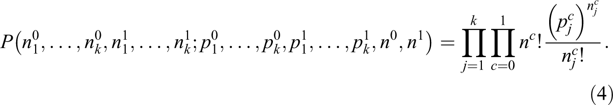
The expectation in equation (5), taken over the independent multinomial distributions with probabilities

where the first two summations run across all possible patterns
Determining Factors
As it has been shown through simulations (see Allen et al. 2009; Carrington and Troske 1997),
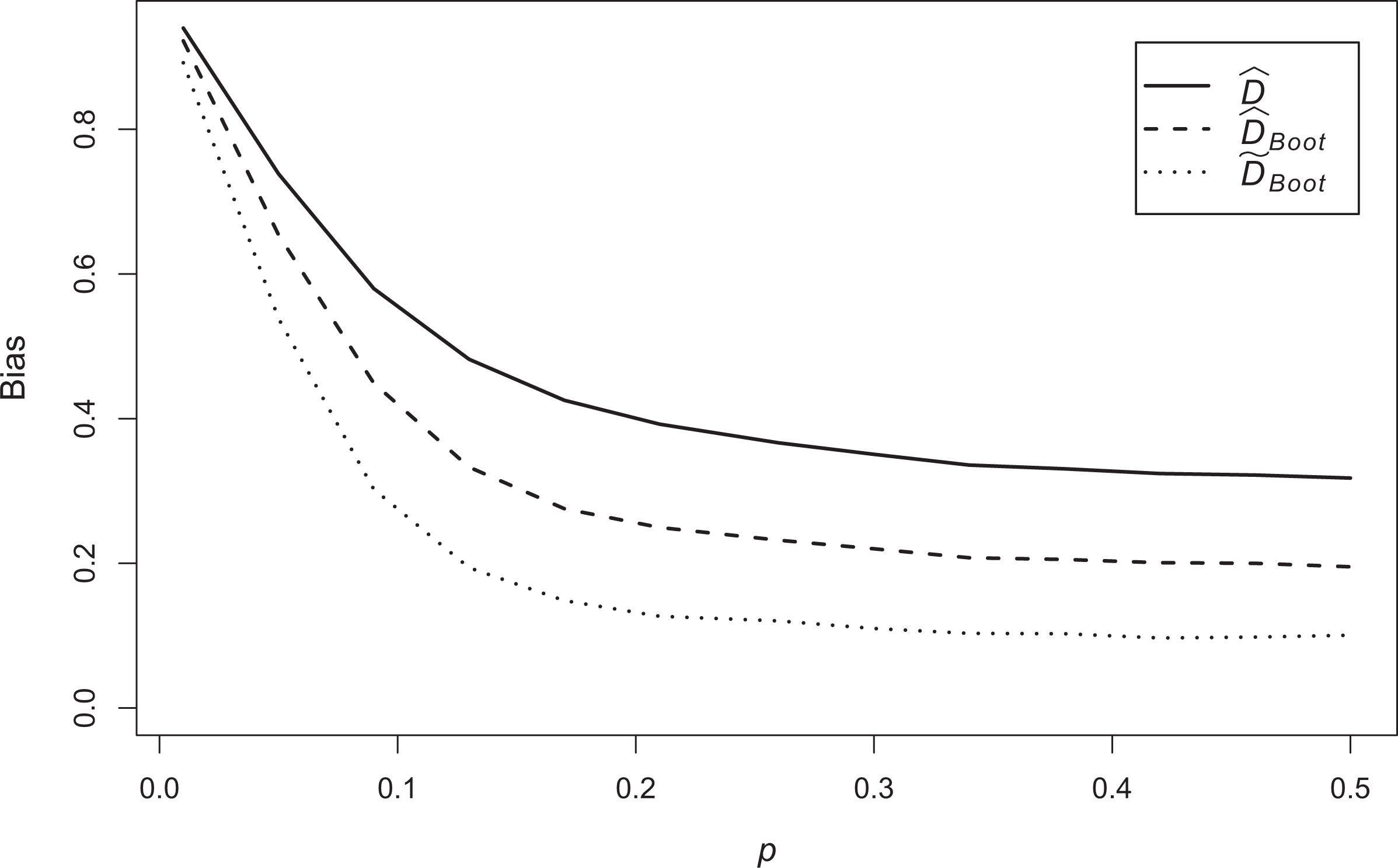
Plots in Figure 1 show the behavior of Behavior of 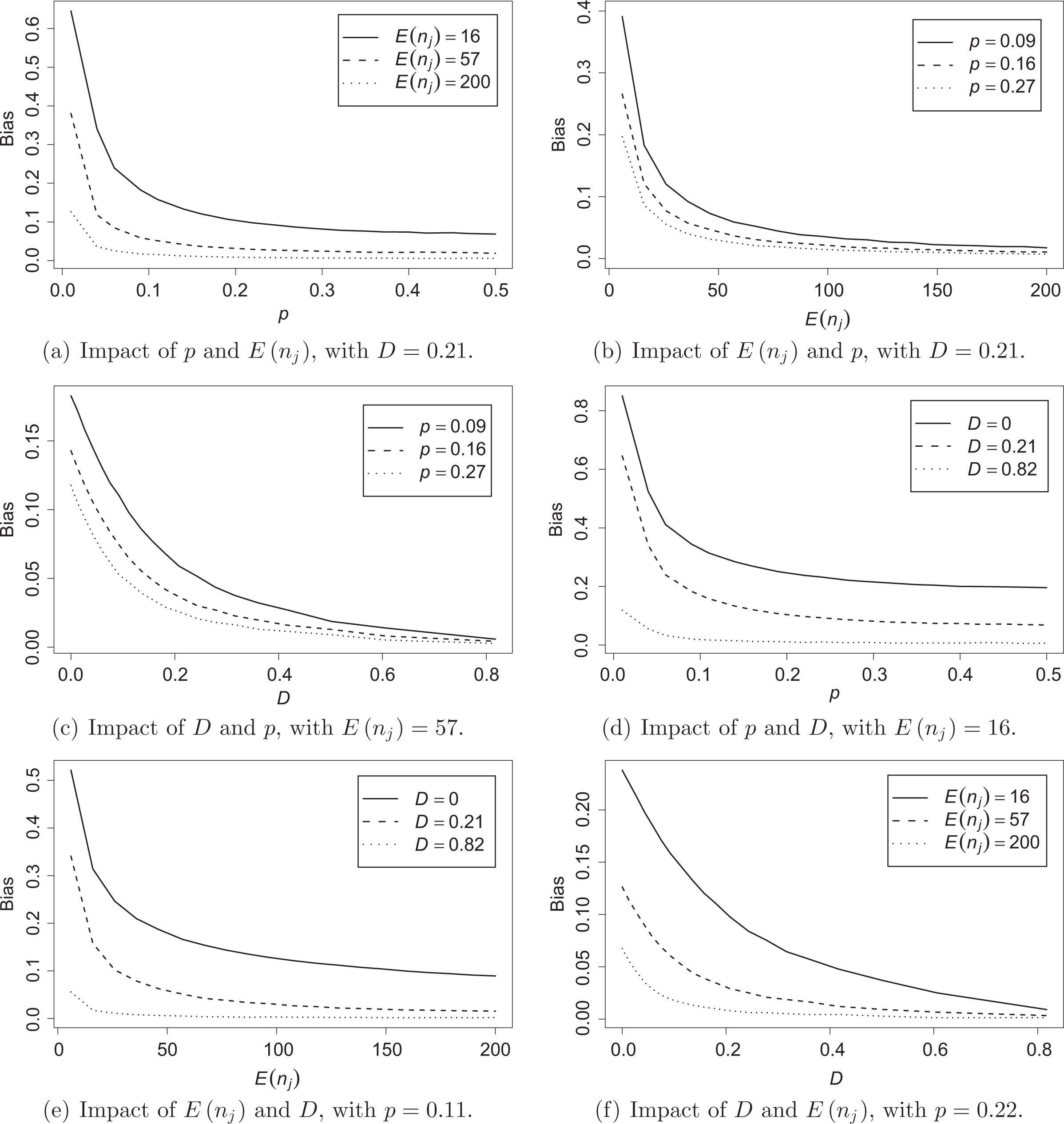

proposed in Duncan and Duncan (1955); it may be observed that each value of q is related to one value of D. Although this set of segregation curves cannot represent all distributions of segregation, it is a sufficient set to examine different levels of systematic segregation for the purposes of this article. Equation (7), combined with the constraint of equal expected unit sizes, fixes the conditional allocation probabilities for both groups. An allocation is then generated assigning n 1 and n 0 individuals to the k units by sampling from two multinomial distributions having each one of the two sets of conditional probabilities as parameter.
Nonnegativity
In the following, we will prove that the nonnegativity of equation (5) can be easily shown reasoning unit by unit.
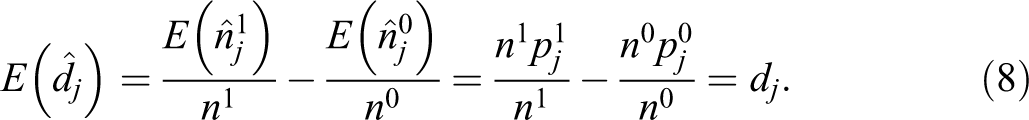
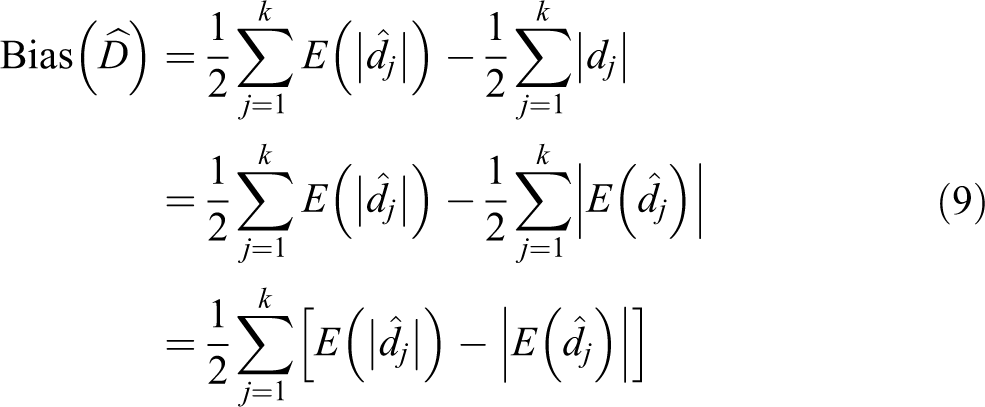
Proof. The allocation mechanism Now, let Thus, using the result in equation (8), equation (5) can be expressed as follows: The quantity in square brackets can be considered as the contribution to the bias given by the jth unit. Being the absolute value, a convex function, from the well-known Jensen’s inequality, we have that

A Bootstrap Bias Correction
With the aim to eliminate, or at least reduce, the upward bias of

where
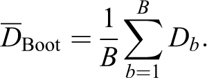
This quantity substitutes the expectation in equation (11). Then, a measure of

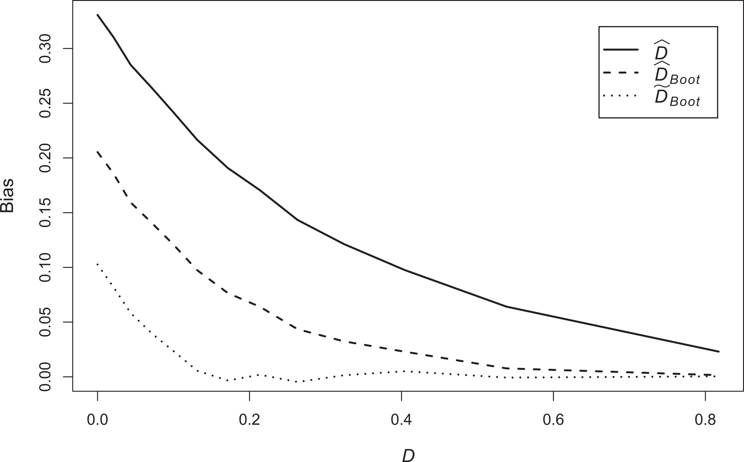
This type of bias correction would work well if the bias were constant for different values of D. This is not the case here, as it is clearly shown in Figure 1c and f. This bias correction is therefore not expected to “eliminate”, but only to “reduce”, the existing bias.
Equivalent Analytical Formulations
Instead of bootstrapping
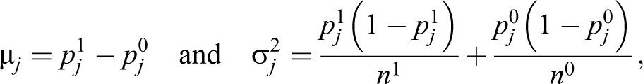
Recall that, considering the generic jth unit,
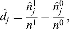
with

Thus, by using the rationale of equation (12), we can define the estimator
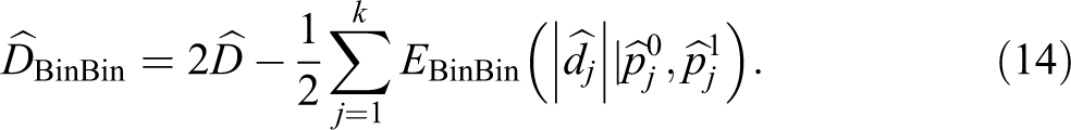
Computation required by equation (14) is easier than equation (6), but it may still be demanding when group size nc
, c = 0, 1, is large. To handle these cases, we propose the following approach.
Proof. As previously said, whose mean results where
According to the rationale of equations (12) and (14) and based on equation (15), we can define the estimator

Comparison
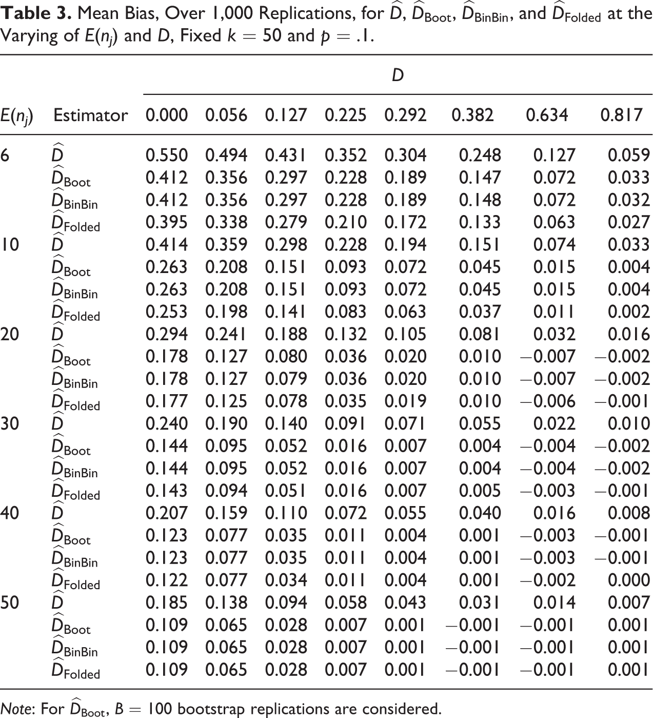
In this section, we use Monte Carlo simulations to compare the bias of the three estimators
Following the setup used for simulations in Determining Factors subsection, the factors considered are as follows: p, E(nj
), and D. For each of them, a grid of values is chosen as follows: 0.01, 0.05, 0.10, 0.30, and 0.50 for p, 6, 10, 20, 30, 40, and 50 for E(nj
), and 0, 0.056, 0.127, 0.225, 0.292, 0.382, 0.634, and 0.818 for D. The values chosen for D are, respectively, related to the values 0, 0.2, 0.4, 0.6, 0.7, 0.8, 0.95, and 0.99, of the parameter q in equation (7). The number of units is fixed at k = 50, their sizes nj
are equal in expectation and, for
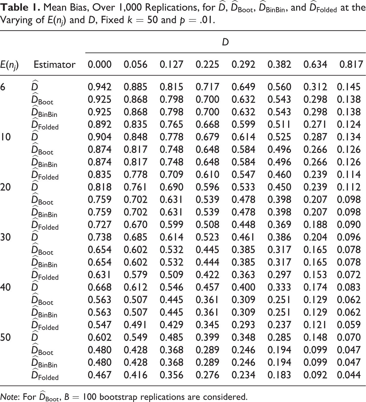
The mean simulated biases of
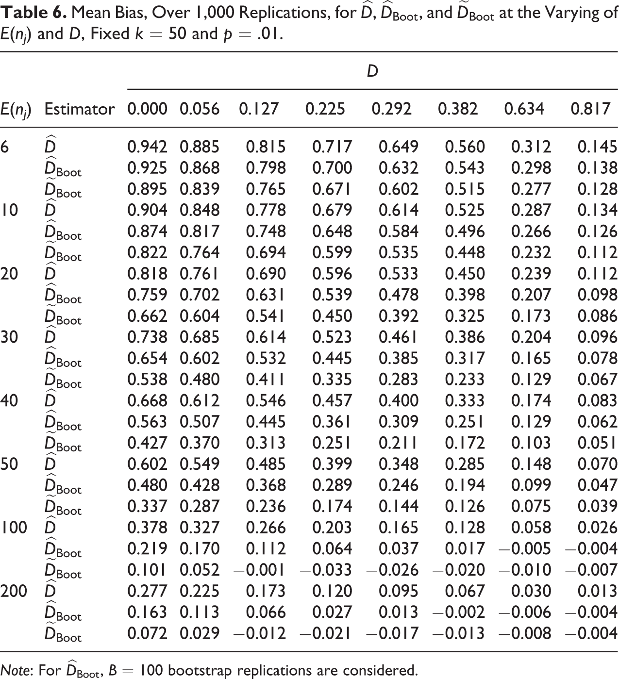
Mean Bias, Over 1000 Replications, for

Note: For
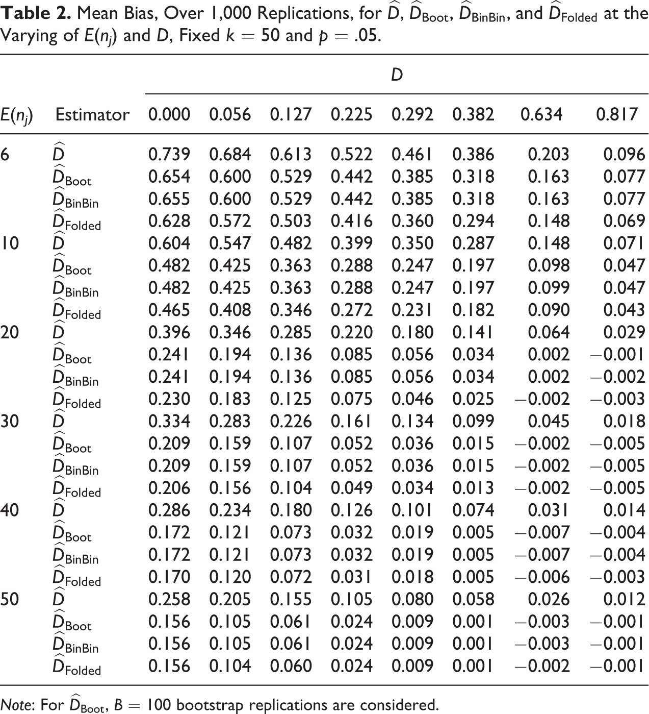
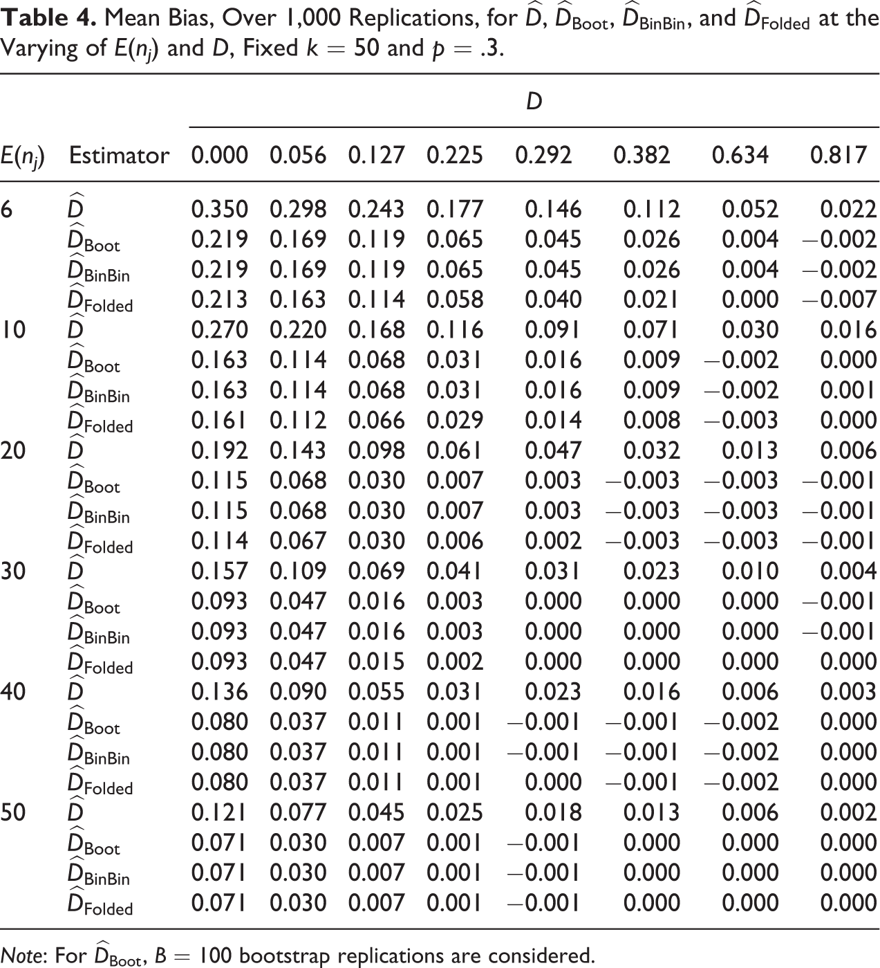
Mean Bias, Over 1,000 Replications, for
Note: For
when p, E(nj
), and D present low values, the observed segregation
in the opposite situation of high values for p, E(nj
), and D, no correction is needed because
for moderate values of D (e.g., from 0.1 to 0.4), provided that p and E(nj
) are not both simultaneously very small,
Comparing
Mean Bias, Over 1,000 Replications, for
Note: For
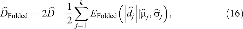
A New Bias Correction
In this section, we introduce a new estimator of D, which further reduces the bias with respect to 
There may be different criteria for choosing
Operationally, an optimization procedure has been implemented in the R computing environment (R Core Team 2013)—available from the authors upon request—that can be summarized as follows. Let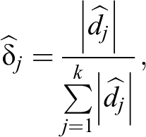
be the relative absolute difference in unit j, j = 1, … , k. For each unit j, we also define the modified probabilities of our estimator as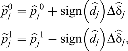
where 
in the range
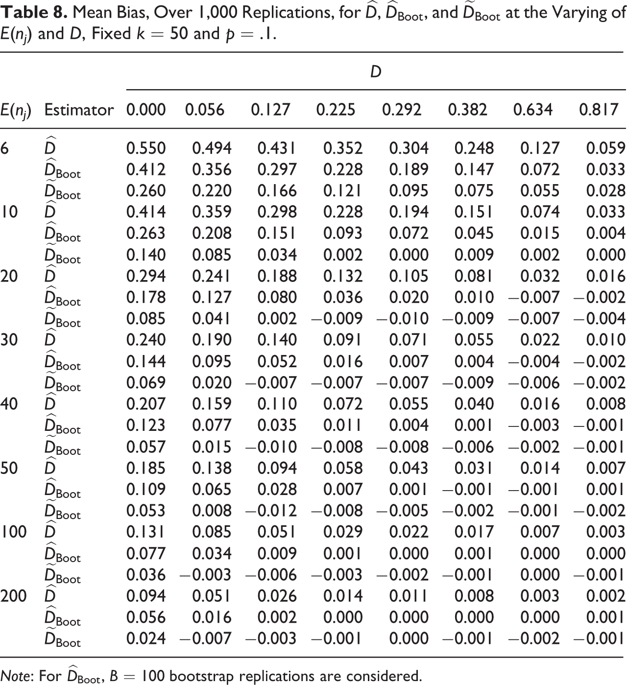
Performance Evaluation
To evaluate the performance of our estimator, we have performed a simulation study having the same design described in the Comparison subsection, but with the addition of the values 100 and 200 for the simulation factor E(nj
). For the sake of brevity, and without loss of generality, only the bootstrap variants
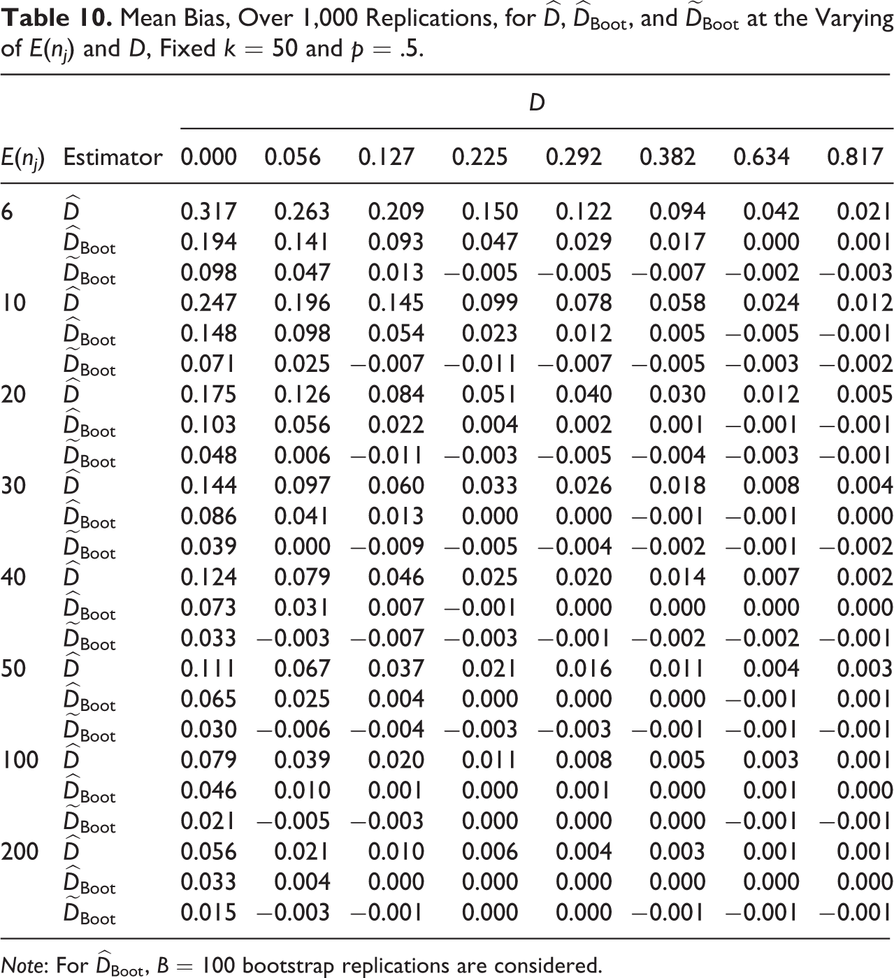
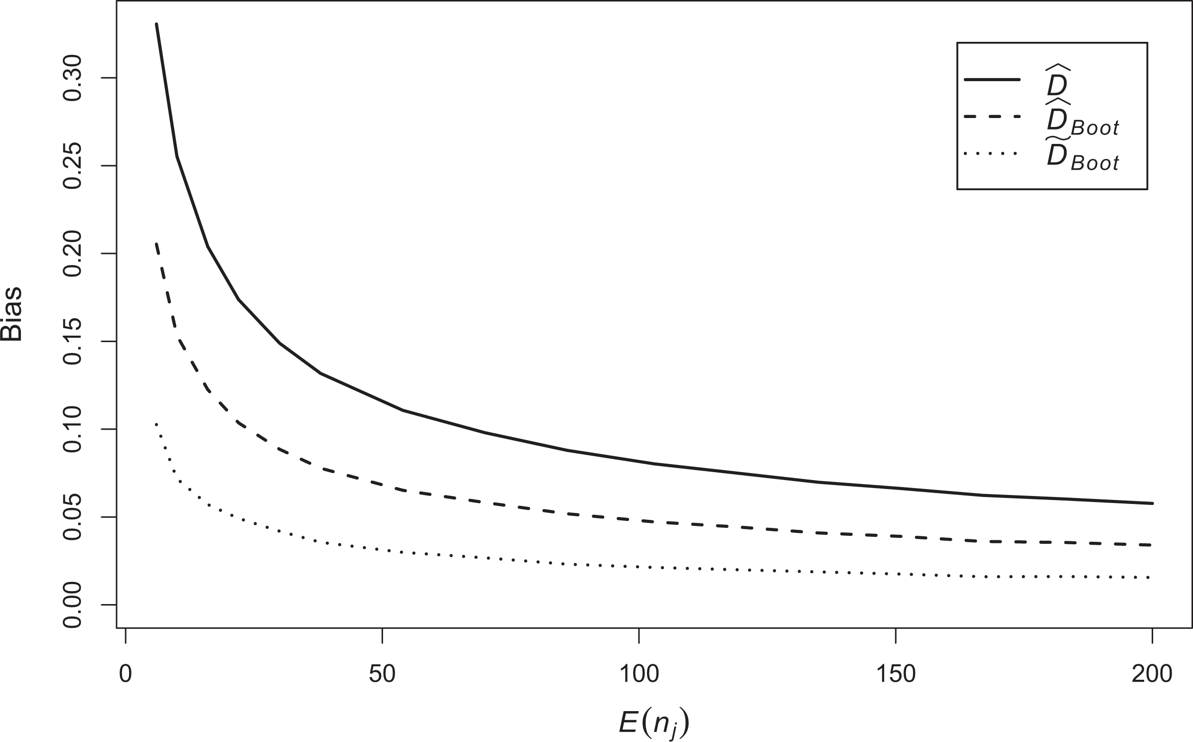
The mean simulated biases of
Comparison between
Comparison between
Mean Bias, Over 1,000 Replications, for
Note: For
Mean Bias, Over 1,000 Replications, for
Note: For
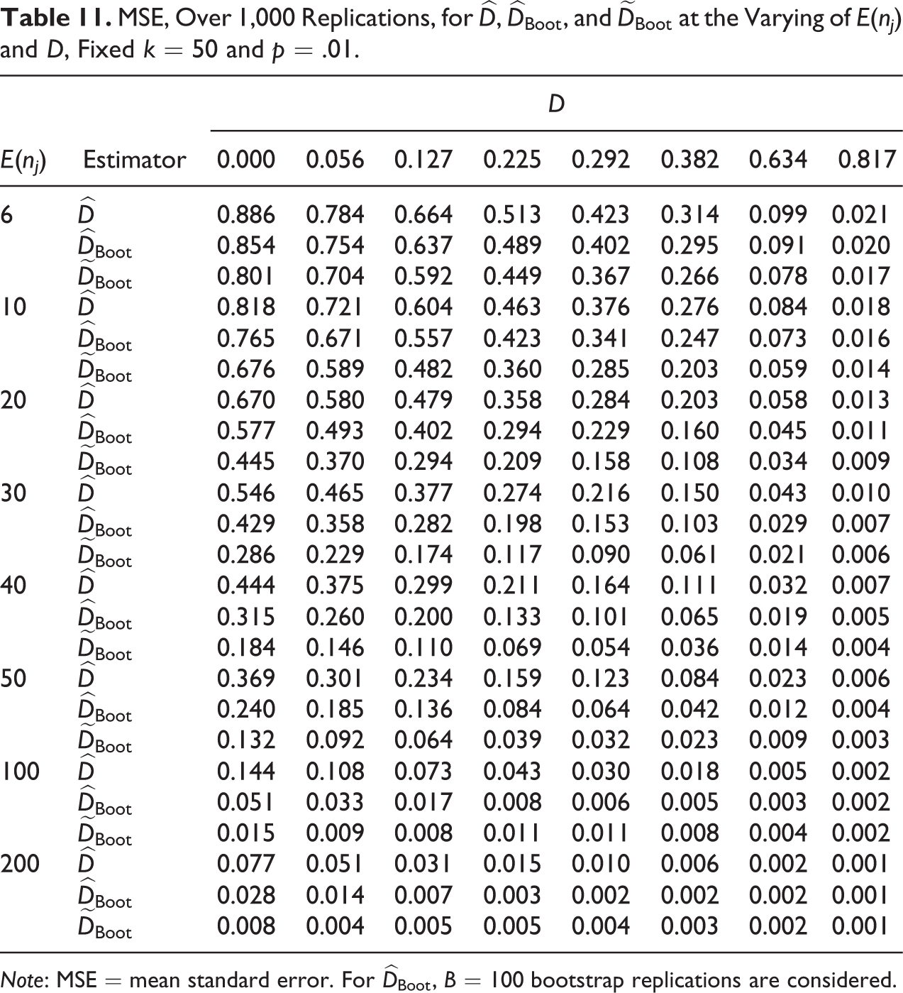
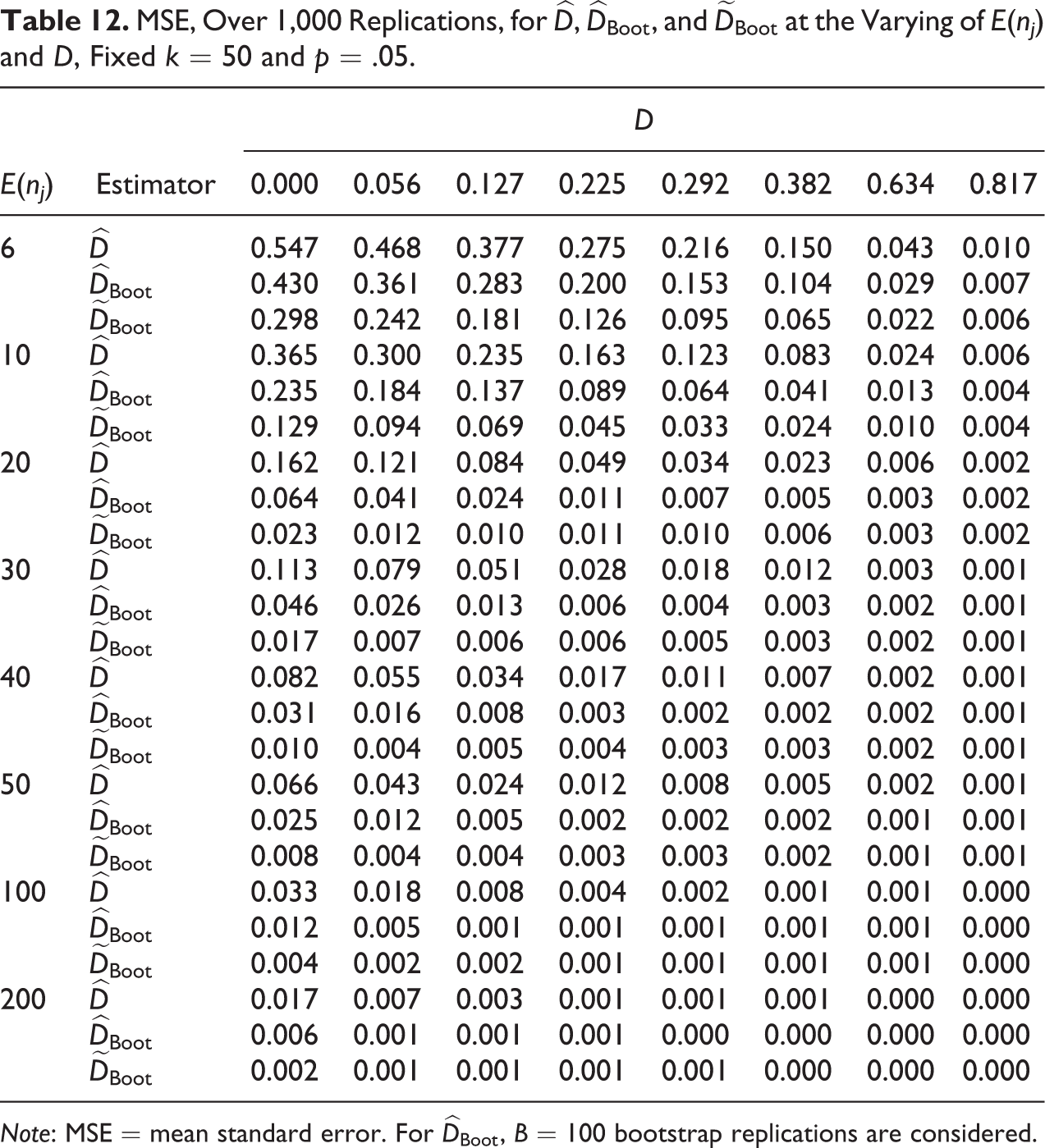
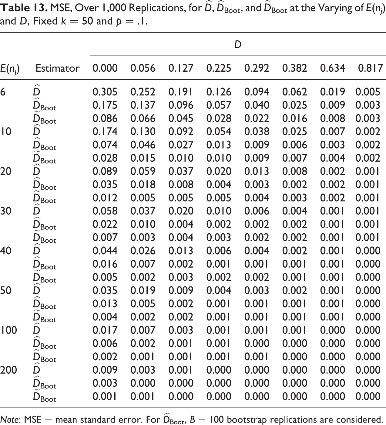
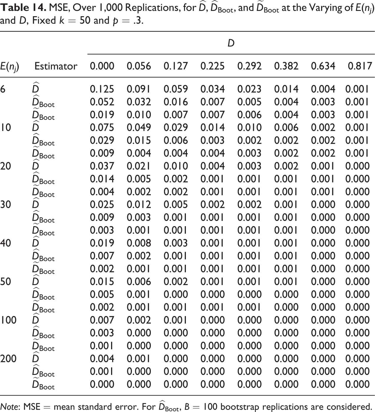
To evaluate the estimation accuracy of the competing estimators, Tables 11
to 15 show the MSEs under the same conditions of Tables 6 to 10. As for the bias,
MSE, Over 1,000 Replications, for
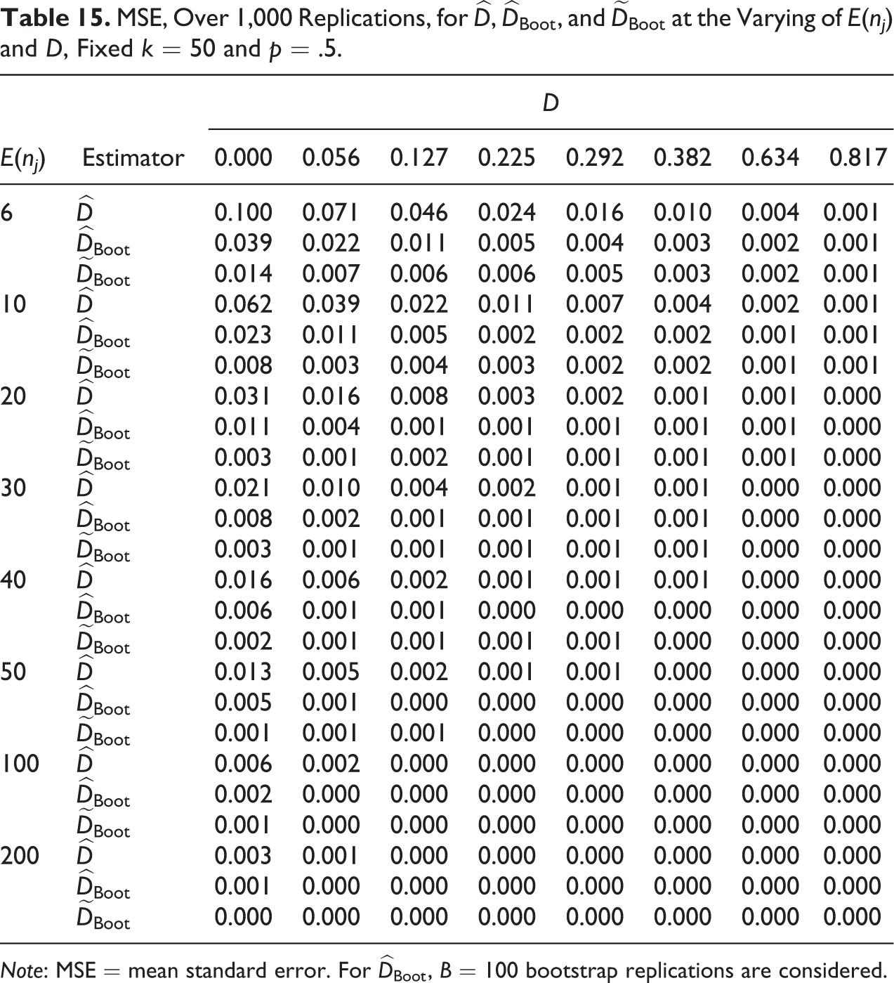
Note: MSE = mean standard error. For
MSE, Over 1,000 Replications, for
Note: MSE = mean standard error. For
We evaluated, also, a grouped jackknife estimator and a double bootstrap estimator; these methods are documented, in their rationale, respectively, in Efron (1982, section 2.2) and Davison and Hinkley (1997, section 3.9). For brevity, tables with mean bias and MSE for these estimators are not reported here but can be obtained from the authors upon request. The grouped jackknife estimator, in all the considered scenarios of simulations, showed only a negligible improvement in mean bias and MSE with respect to
Conclusions
It has long been recognized that the sensitivity of the dissimilarity index of Duncan and Duncan (1955) to random allocation implies an upward bias, particularly evident with smaller unit sizes, small minority proportions, and lower levels of segregation (see, e.g., Carrington and Troske 1997; Cortese et al. 1976; Ransom 2000). In this article, following the multinomial framework of Allen et al. (2009), we have demonstrated analytically the nonnegativity of this bias. Furthermore, we have shown that the same bootstrap-based bias correction introduced by Allen et al. (2009) can be obtained analytically, without resorting to resampling techniques. Finally, we have introduced a new bias correction in simulations that always performed better than the previous one in terms of both mean bias and MSE; nevertheless, for reliable estimations, both minority proportion and unit sizes do not have to be very small. Alternative estimators, based on grouped jackknife and double bootstrap, have also been evaluated, in terms of both mean bias and MSE. The grouped jackknife bias-corrected estimator exhibited only a little improvement over the natural estimator and so did the double bootstrap estimator with respect to the bootstrap bias-corrected one. Our bias correction procedure has been implemented in the R language and may be requested to the authors.
Comparison between
Mean Bias, Over 1,000 Replications, for
Note: For
Mean Bias, Over 1,000 Replications, for
Note: For
Mean Bias, Over 1,000 Replications, for

Note: For
Mean Bias, Over 1,000 Replications, for
Note: For
Mean Bias, Over 1,000 Replications, for

Note: For
MSE, Over 1,000 Replications, for
Note: MSE = mean standard error. For
MSE, Over 1,000 Replications, for
Note: MSE = mean standard error. For
MSE, Over 1,000 Replications, for
Note: MSE = mean standard error. For
Footnotes
Declaration of Conflicting Interests
The author(s) declared no potential conflicts of interest with respect to the research, authorship, and/or publication of this article.
Funding
The author(s) received no financial support for the research, authorship, and/or publication of this article.