Causes of Effects and Effects of Causes

Abstract

This article summarizes a conceptual framework and simple mathematical methods of estimating the probability that one event was a necessary cause of another, as interpreted by lawmakers. We show that the fusion of observational and experimental data can yield informative bounds that, under certain circumstances, meet legal criteria of causation. We further investigate the circumstances under which such bounds can emerge, and the philosophical dilemma associated with determining individual cases from statistical data.

Keywords

probability of necessity probability of causation counterfactuals legal liability attribution

Introduction

I am grateful to the editors for inviting me to comment on the article by Dawid, Fienberg, and Faigman (2014; henceforth DFF), in which they justifiably emphasize the fundamental distinction between “Effect of Causes” (EoC) and “Causes of Effect” (CoE).

My aim in this comment is to share with readers a progress report on what has been accomplished on the question of CoEs, how far we have come in using population data to decide individual cases and how well we can answer questions that lawmakers ask about individual’s liability. I hope this account convinces readers that the analysis of CoEs has not lagged behind that of EoC. Both modes of reasoning enjoy a solid mathematical basis, endowed with powerful tools of analysis, and researchers on both fronts now possess solid understanding of applications, identification conditions, and estimation techniques.

The Logic of Counterfactuals

A good place to start is the mathematization of counterfactuals, a development that is responsible, at least partially, for legitimizing counterfactuals in scientific discourse,¹ and which has reduced the quest for CoEs to an exercise in logic (Pearl 2011).

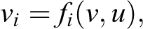
At the center of this logic lies a model, M, consisting of a set of equations similar to those used by physicists, geneticists (Wright 1921), economists (Haavelmo 1943), and social scientists (Duncan 1975) to articulate scientific knowledge in their respective domains. M consists of two sets of variables, U and V, and a set F of equations that determine how values are assigned to each variable $V_{i} \in V$ . Thus, for example, the equation

v_{i} = f_{i} (v, u),

describes a physical process by which nature examines the current values, v and u, of all variables in V and U and, accordingly, assigns variable V_i the value v_i = f_i (v, u). The variables in U are considered “exogenous,” namely, background conditions for which no explanatory mechanism is encoded in model M. Every instantiation U = u of the exogenous variables corresponds to defining a “unit,” or a “situation” in the model, and uniquely determines the values of all variables in V. Therefore, if we assign a probability P(u) to U, it defines a probability function P(v) on V. The probabilities on U and V can best be interpreted as the proportion of the population with a particular combination of values on U and/or V.

The basic counterfactual entity in structural models is the sentence: “Y would be y had X been x in situation U = u,” denoted Y_x (u) = y, where Y and X are any variables in V. The key to interpreting counterfactuals is to treat the subjunctive phrase “had X been x ” as an instruction to make a minimal modification in the current model, so as to ensure the antecedent condition X = x. Such a minimal modification amounts to replacing the equation for X by a constant x, which may be thought of as an external intervention do(X = x), not necessarily by a human experimenter that imposes the condition X = x. This replacement permits the constant x to differ from the actual value of X, namely, f_x (v, u), without rendering the system of equations inconsistent, thus allowing all variables, exogenous as well as endogenous, to serve as antecedents.

Letting M_x stand for a modified version of M, with the equation/equations of X replaced by X = x, the formal definition of the counterfactual Y_x (u) reads (Balke and Pearl 1994a,1994b):

Y_{x} (u) \overset{Δ}{=} Y_{M_{x}} (u) .

In words, the counterfactual Y_x (u) in model M is defined as the solution for Y in the “surgically modified” submodel M_x . Galles and Pearl (1998) and Halpern (1998) have given a complete axiomatization of structural counterfactuals, embracing both recursive and nonrecursive models (see also Pearl 2009:chap. 7). They showed that the axioms governing recursive structural counterfactuals are identical to those used in the potential outcomes framework, hence the two systems are logically identical—a theorem in one is a theorem in the other. This means that relying on structural models as a basis for counterfactuals does not impose additional assumptions beyond those routinely invoked by potential outcome practitioners. Consequently, going from effects to causes does not require extra mathematical machinery beyond that used in going from causes to effects.

Since our model M consists of a set of structural equations, it is possible to calculate probabilities that might at first appear nonsensical. As noted earlier, the probability distribution on U, P(u) induces a well-defined probability distribution on V, P(v). As such, it not only defines the probability of any single counterfactual, Y_x = y, but also the joint distribution of all conceivable counterfactuals. As also noted earlier, these probabilities refer to the proportion of individuals in the population with specific counterfactual values that may or may not be observed. Thus, the probability of the Boolean combination, “Y_x = y AND Z_x′ = z” for variables Y and Z in V and two different values of X, x, and x′, is well defined even though it is impossible for both outcomes to be simultaneously observed as X = x and X = x′ cannot be concurrently true.

To answer CoE-type questions, such as “if X were x ₁ would Y be y ₁ for individuals for whom in fact X is Y _x
₁ and Y is y ₀,” we need to compute the conditional probability P(Y _x
₁ = y ₁ | Y = y ₀, X = x ₀); (Balke and Pearl 1994a, 1994b). This probability, that is, the proportion of the population with this combination of counterfactual values, is well defined once the structural equations and the distribution of exogenous variables, U, is known.

In general, the probability of the counterfactual sentence P(Y _x = y | e), where e is any information about an individual, can be computed by the three-step process:

Step 1 (abduction): Update the probability P(u) to obtain P(u | e).

Step 2 (action): Replace the equations corresponding to variables in set X by the equation X = x.

Step 3 (prediction): Use the modified model to compute the probability of Y = y.

In temporal metaphors, step 1 explains the past (U) in light of the current evidence e; step 2 bends the course of history (minimally) to comply with the hypothetical antecedent X = x; finally, step 3 predicts the future (Y) based on our new understanding of the past and our newly established condition, X = x.

Pearl (2009:296-99, 2012) gives several examples illustrating the simplicity of this computation and how CoE-type questions can be answered when the model M is known. If M is not known, but is assumed to take a parametric form, one can use population data to estimate the parameters and, subsequently, all counterfactual queries can be answered, including those that pertain to causes of individual cases (Pearl 2009:389-91; 2012). Thus, the challenge of reasoning from group data to individual cases has been met.

When the model M is not known, we can prove that, in general, probabilities of causes are not identifiable from experimental or observational data. However, using group data with observations about an individual, tight bounds can be derived, which can be quite informative. We will illustrate these bounds as an example taken from judicial context similar to the one considered by DFF.

Legal Liability from Experimental and Nonexperimental Data

A lawsuit is filed against the manufacturer of drug x, charging that the drug is likely to have caused the death of Mr. A, who took the drug to relieve back pains. The manufacturer claims that experimental data on patients with back pains show conclusively that drug x may have only minor effect on death rates. However, the plaintiff argues that the experimental study is of little relevance to this case because it represents average effects on all patients in the study, not on patients like Mr. A who did not participate in the study. In particular, argues the plaintiff, Mr. A is unique in that he used the drug on his own volition, unlike subjects in the experimental study who took the drug to comply with experimental protocols. To support this argument, the plaintiff furnishes nonexperimental data on patients who, like Mr. A, chose drug x to relieve back pains, but were not part of any experiment. The court must now decide, based on both the experimental and the nonexperimental studies, whether it is “more probable than not” that drug x was in fact the cause of Mr. A’s death.

This example falls under the category of CoEs because it concerns situation in which we observe both the effect, Y = y, and the putative cause X = x and we are asked to assess, counterfactually, whether the former would have occurred absent the latter.

Assuming binary events, with X = x and Y = y representing treatment and outcome, respectively, and X = x′, Y = y′ their negations, our target quantity can be formulated directly from the English sentence:

Find the probability that if X had been x′, Y would be y′, given that, in reality, X is x and Y is y.

to give:

P N (x, y) = P (Y_{x^{'}} = y^{'} | X = x, Y = y) .

This counterfactual quantity, which Robins and Greenland (1989) named “probability of causation” (PC) and Pearl (2000a:296) named “probability of necessity” (PN), to be distinguished from two other nuances of “causation,” captures the “but for” criterion according to which judgment in favor of a plaintiff should be made if and only if it is “more probable than not” that the damage would not have occurred but for the defendant’s action (Robertson 1997). In contrast, the PC measure proposed by Dawid, Fienberg, and Faigman:

P C = P (Y_{x^{'}} = y^{'} | Y_{x} = y),

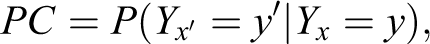
represents the probability that a person who took the drug under experimental conditions and died, Y_x = y, would be alive had he not been assigned the drug, Y_x _′ = y′. It thus represents the probability that the drug was the cause of death of a subject who died in the experimental setup. Very few court cases deal with deaths under experimental circumstances; most deal with deaths, damage, or injuries that took place under natural, every day conditions, for which the DFF’s measure is inapplicable.

Having written a formal expression for PN, equation (2), we can move on to the identification phase and ask what assumptions would permit us to identify PN from empirical studies, be they observational, experimental, or a combination thereof.

This problem is analyzed in Pearl (2000a:chap. 9) and yields the following results:

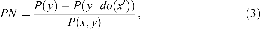
Theorem 1: If Y is monotonic relative to X, that is, $Y_{1} (u) \geq Y_{0} (u)$ , then PN is identifiable whenever the causal effect $P (y | d o (x))$ is identifiable and, moreover,

P N = \frac{P (y) - P (y | d o (x^{'}))}{P (x, y)},

or,²

P N = \frac{P (y | x) - P (y | x^{'})}{P (y | x)} + \frac{P (y | x^{'}) - P (y | d o (x^{'}))}{P (x, y)} .

The first term on the right-hand side of equation (4) is the familiar excess risk ratio (ERR) that epidemiologists have been using as a surrogate for PN in court cases (Cole 1997; Greenland 1999; Robins and Greenland 1989). The second term represents a correction needed to account for confounding bias, that is, $P (y | d o (x^{'})) \neq P (y | x^{'})$ or, put in words, when the proportion of population for whom Y = y when X is set to x′ for everyone is not the same as the proportion of the population for whom Y = y among those observed to acquire the value X = x′.

Equation (4) thus provides a more refined measure of causation, which can be used for monotonic Y_x (u) whenever the causal effect $P (y | d o (x))$ can be estimated, from either randomized trials or graph-assisted observational studies (e.g., through the back-door criterion, Pearl 1993, or the do-calculus). More significantly, it has also been shown (Tian and Pearl 2000) that the expression in equation (3) provides a lower bound for PN in the general, nonmonotonic case. In particular, the tight upper and lower bounds on PN are given by:

max \{0, \frac{P (y) - P (y | d o (x^{'}))}{P (x, y)}\} \leq P N \leq min \{1, \frac{P (y^{'} | d o (x^{'})) - P (x^{'}, y^{'})}{P (x, y)}\} .

In drug-related litigation, it is not uncommon to obtain data from both experimental and observational studies. The former is usually available at the manufacturer or the agency that approved the drug for distribution (e.g., Food and Drug Administration ), while the latter is easy to obtain by random surveys of the population. 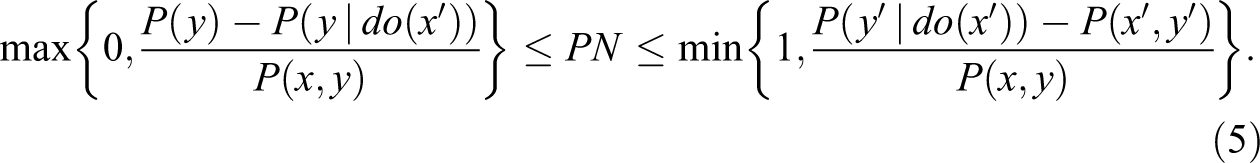If it is the case that the experimental and survey data have been drawn at random from the same population, then the experimental data can be used to estimate the counterfactuals of interest, for example, P(Y_x = y) for the observational and experimental sampled populations. In such cases, the standard lower bound used by epidemiologists to establish legal responsibility, the ERR, can be improved substantially using the corrective term of equation (4). Likewise, the upper bound of equation (5) can be used to exonerate drugmakers from legal responsibility. Remarkably, regardless of confounding the gap between the upper and the lower bounds is constant and is given by one observable parameter, $P (y^{'} | x) / P (y | x)$ (Pearl 2014). Cai and Kuroki (2006) analyzed the finite-sample properties of PN. Yamamoto (2012) used instrumental variables to derive similar bounds for subpopulations permitting effect identification.

Numerical Example

To illustrate the usefulness of the bounds in equation (5), consider the (hypothetical) data associated with the two studies shown in Table 1. (In the subsequent analyses, we ignore sampling variability, that is, we assume that our population is of infinite size.)

Table 1.

Experimental and Nonexperimental Data used to illustrate the estimation of PN, the probability that drug x was responsible for a person's death (y).

	Experimental		Nonexperimental
	do(x)	do(x′)	x	x′
Deaths (y)	16	14	2	28
Survivals (y′)	984	986	998	972

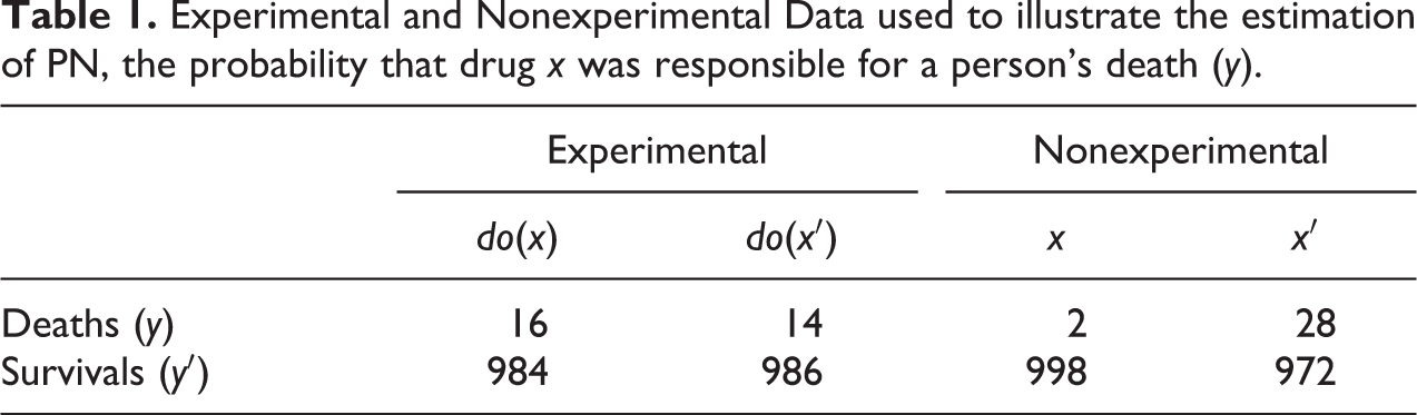
The experimental data provide the estimates

P (y | d o (x)) = 16 / 1, 000 = 0.016,

P (y | d o (x^{'})) = 14 / 1, 000 = 0.014;

while the nonexperimental data provide the estimates

P (y) = 30 / 2, 000 = 0.015,

P (y, x) = 2 / 2, 000 = 0.001,

P (y | x) = 2 / 1, 000 = 0.002,

P (y | x^{'}) = 28 / 1, 000 = 0.028.

Assuming that drug x can only cause (but never prevent) death, monotonicity holds and Theorem 1 (equation 4) yields

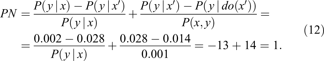
\begin{aligned} P N = \frac{P (y | x) - P (y | x^{'})}{P (y | x)} + \frac{P (y | x^{'}) - P (y | d o (x^{'}))}{P (x, y)} = \\ = \frac{0.002 - 0.028}{P (y | x)} + \frac{0.028 - 0.014}{0.001} = - 13 + 14 = 1. \end{aligned}

We see that while the observational ERR is negative (−13), giving the impression that the drug is actually preventing deaths, the bias correction term (+14) rectifies this impression and sets the PN to unity. Moreover, since the lower bound of equation (5) becomes 1, we conclude that PN = 1.00 even without assuming monotonicity. Thus, the plaintiff was correct; barring sampling errors, these data provide us with 100 percent assurance that drug x was in fact responsible for the death of Mr. A. Note that DFF’s proposal of using the experimental ERR 1 − 1/RR would yield a much lower result:

\frac{P (y | d o (x)) - P (y | d o (x^{'}))}{P (y | d o (x))} = \frac{0.016 - 0.014}{0.016} = 0.125,

which does not meet the “more probable than not” requirement.³

What the experimental study does not reveal is that, given a choice, terminal patients tend to avoid drug x, that is, the 14 patients in the experimental study who did not take the drug and died anyway would have avoided the drug if they were in the nonexperimental study. In fact, as our earlier analysis shows, there are no terminal patients who would choose x (given the choice). If there were terminal patients that would choose x, given the choice, then by randomization some of these patients (50 percent in our example) would be in the control group in the experimental data. As a result, the proportion of deaths in the control group in the experimental data, P(y_x _′), would be higher than the proportion of terminal patients in the nonexperimental data, P(y, x′). However, examining the data in our hypothetical example, we observe that P(y | do(x′)) = P(y, x′) = .0014, implying that there are no terminal patients in the nonexperimental data who chose the treatment condition. As such, any individual in the nonexperimental data who chose the treatment and died must have died because of the treatment as they were not terminal.

The numbers in Table 1 were obviously contrived to represent an extreme case and so facilitate a qualitative explanation of the validity of equation (12). Nevertheless, it illustrates decisively that a combination of experimental and nonexperimental studies may unravel what experimental studies alone will not reveal and, in addition, that such combination may provide a necessary test for the adequacy of the experimental procedures. For example, if the frequencies in Table 1 were slightly different, they could easily yield a PN value greater than unity in equation (12), thus violating consistency, $P (y | d o (x)) \geq P (x, y)$ . Such violation must be due to incompatibility of experimental and nonexperimental groups, or an improperly conducted experiment.

This last point may warrant a word of explanation, lest the reader wonder why two data sets—taken from two separate groups under different experimental conditions—should constrain one another. The explanation is that certain quantities in the two subpopulations are expected to remain invariant to all these differences, provided that the two subpopulations were sampled randomly from the population at large. These invariant quantities are simply the causal effects probabilities, $P (y | d o (x^{'}))$ and $P (y | d o (x))$ . Although these probabilities were not measured in the observational group, they must nevertheless be the same as those measured in the experimental group (ignoring differences due to sampling variability). The invariance of these quantities implies the inequalities of equation (5).

The example of Table 1 shows that combining data from experimental and observational studies which, taken separately, may indicate no causal relations between X and Y, can nevertheless bring the lower bound of equation (5) to unity, thus implying causation with probability approaching one.

Such extreme results demonstrate that a counterfactual quantity PN which at first glance appears to be hypothetical, ill-defined, untestable and, hence, unworthy of scientific analysis is nevertheless definable, testable and, in certain cases, for example, when monotonicity holds, even identifiable. Moreover, the fact that, under certain combinations of data and making no assumptions whatsoever, an important legal claim such as “the plaintiff would be alive had he not taken the drug” can be ascertained with probability approaching one, is a remarkable tribute to formal analysis.⁴

How Informative Are the PN Bounds?

To see how informative the bounds are, and how sensitive they are to variations in the experimental and observational data, consider the following example. Assume that the population of patients contains a fraction r of individuals who suffer from a certain death-causing syndrome Z, which simultaneously makes it uncomfortable for them to take the drug. Referring to Figure 1, let Z = z ₁ and Z = z ₀ represent, respectively, the presence and absence of the syndrome, Y = y ₁ and Y = y ₀ represent death and survival, respectively, and X = x ₁ and X = x ₀ represent taking and not taking the drug, respectively. Assume that patients carrying the syndrome, Z = z ₁, are terminal cases, for whom death occurs with probability 1, regardless of whether they take the drug. Patients not carrying the syndrome, on the other hand, incur death with probability p ₂ if they take the drug and with probability p ₂ if they don’t take. We will further assume p ₂ > p ₁ so that the drug appears to be a risk factor for ordinary patients and that patients having the syndrome are more likely to avoid the drug; that is, q ₂ < q ₁ where $q_{1} = P (x_{1} | z_{0})$ and $q_{2} = p (x_{1} | z_{1})$ .

Figure 1.

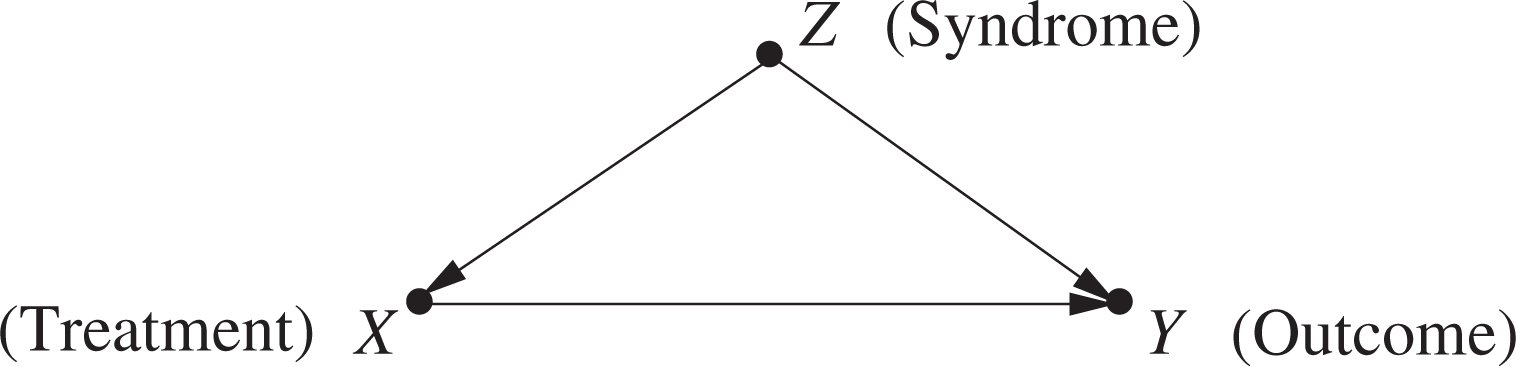
Model generating the experimental and observational data of equations (16 and 17). Z represents an unobserved confounder affecting both treatment (X) and outcome (Y).

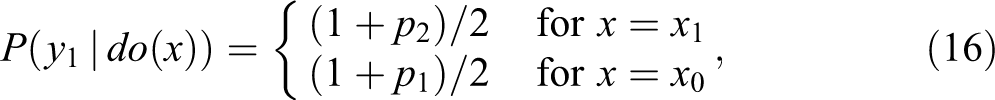
Based on this model, we can compute the causal effect of the drug on death using:

P (y | d o (x)) = \sum_{z} P (y | x, z) P (z) f o r a l l y a n d x,

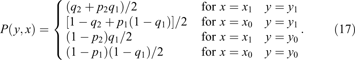
and the joint distribution P(x, y) using:

P (y, x) = \sum_{z} P (y | x, z) P (x | z) P (z) f o r a l l y, x .

Substituting the model’s parameters and assuming r = 1/2 gives:

P (y_{1} | d o (x)) = \{\begin{matrix} (1 + p_{2}) / 2 & f o r x = x_{1} \\ (1 + p_{1}) / 2 & f o r x = x_{0} \end{matrix},

P (y, x) = \{\begin{matrix} (q_{2} + p_{2} q_{1}) / 2 & f o r x = x_{1} y = y_{1} \\ [1 - q_{2} + p_{1} (1 - q_{1})] / 2 & f o r x = x_{0} y = y_{1} \\ (1 - p_{2}) q_{1} / 2 & f o r x = x_{1} y = y_{0} \\ (1 - p_{1}) (1 - q_{1}) / 2 & f o r x = x_{0} y = y_{0} \end{matrix} .

Accordingly, the bounds of equation (5) become:

(p_{2} - p_{1}) / (p_{2} + q_{2} / q_{1}) \leq P N \leq (1 - p_{1}) / (p_{2} + q_{2} / q_{1}) .

Equating the upper and lower bounds in equation (18) reveals that PN is identified if and only if q ₁(1 − p ₂) = 0, namely, if patients carrying the syndrome either do not take the drug or do not survive if they do. For intermediate value of p ₂ and q ₁, PN is constrained to an interval that depends on all four parameters.

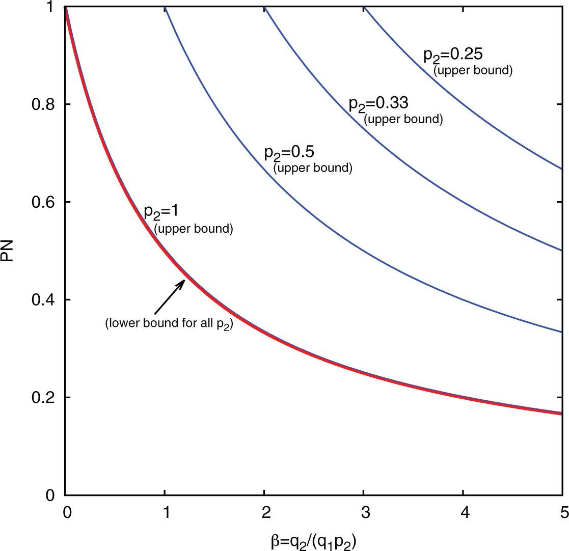
Figure 2 displays the lower bound (red curve) as a function of the parameter $β = q_{2} / q_{1} p_{2}$ , for p ₁ = 0 and the upper bounds (green curves) for p ₂ = 1.00, 0.5, 0.33, and 0.25. We see that lower bound approaches 1 when q ₂ approaches zero, while the upper bounds are situated a factor 1/p ₂ above the lower bound. A more elaborate visualization of these bounds is given in Pearl (2014).

Figure 2.

Showing the lower bound of probability of necessity (PN) for p ₁ = 0 (red curve) and several upper bounds (blue curves).

Is “Guilty With Probability One” Ever Possible?

People tend to disbelieve this possibility for two puzzling aspects of the problem:

that a hypothetical, generally untestable quantity can be ascertained with probability one under certain conditions;

that a property of an untested individual can be assigned a probability one based on the data taken from sampled population.

The first puzzle is not really surprising for students of science who take seriously the benefits of logic and mathematics. Once we give a quantity formal semantics, we essentially define its relation to the data, and it is not inconceivable that data obtained under certain conditions would sufficiently constrain that quantity, to a point where it can be determined exactly.

The second puzzle is the one that gives most people a shock of disbelief. For a statistician, in particular, it is a rare case to be able to say anything certain about a specific individual who was not tested directly. This emanates from two factors. First, statisticians normally deal with finite samples, the variability of which rules out certainty in any claim, not merely about an individual but also about any property of the underlying distribution. This factor, however, should not enter into our discussion, for we have been assuming infinite samples throughout. (Readers should imagine that the numbers in Table 1 stand for millions.)

The second factor emanates from the fact that, even when we know a distribution precisely, we cannot assign a definite probabilistic estimate to a property of a specific individual drawn from that distribution. The reason is, so the argument goes, that we never know, let alone measure, all the anatomical and psychological variables that determine an individual’s behavior, and, even if we knew, we would not be able to represent them in the crude categories provided by the distribution at hand. Thus, because of this inherent crudeness, the sentence “Mr. A would be dead” can never be assigned a probability one (or, in fact, any definite probability).

This argument, advanced by Freedman and Stark (1999) is incompatible with the way probability statements are used in ordinary discourse, for it implies that every probability statement about an individual must be a statement about a restricted subpopulation that shares all the individual’s characteristics. Taken to extreme, such restrictive interpretation would insist on characterizing the plaintiff to minute detail and would reduce the “but for” probability to zero or one when all relevant details are accounted for. It is inconceivable that this interpretation underlies the intent of judicial standards. By using the wording “more probable than not,” lawmakers have instructed us to ignore specific features that are either irrelevant or for which data are not likely to be available, and to base our determination on the most specific yet essential features for which data are expected to be available. In our example, two properties of Mr. A were noted: (1) that he died and (2) that he chose to use the drug; these are essential and were properly taken into account in bounding PN. In certain court cases, additional characteristics of Mr. A would be deemed essential. For example, it is quite reasonable that, in the case of Mr. A, the court may deem his medical record to be essential, in which case, the analysis should proceed by restricting the reference class to subjects with medical history similar to that of Mr. A. However, having satisfied such specific requirements, and knowing in advance that we will never be able to match all the idiosyncratic properties of Mr. A, the lawmakers’ intent must be interpreted relative to the probability bounds provided by PN.

Conclusions

I agree with DFF that the issues surrounding reasoning from EoC to CoE involve the challenge of reasoning from group data to individual cases. However, the logical gulf between the two is no longer a hindrance to systematic analysis. It has been bridged by the structural semantics of counterfactuals (Balke and Pearl 1994a, 1994b) and now yields a coherent framework of fusing experimental and observational data to decide individual cases of all kinds, CoE included.

I invite Dawid, Fienberg, and Faigman to reap the benefits and opportunities unleashed by the counterfactual theory of CoE.

Footnotes

Acknowledgment

I am grateful to Nicholas Jewell and the editor of Sociological Methods and Research for calling my attention to the DFF's paper, and for helpful comments on the first version of the manuscript. Portions of this paper are based on Pearl (2000a, 2011, 2012).

Declaration of Conflicting Interests

The author(s) declared no potential conflicts of interest with respect to the research, authorship, and/or publication of this article.

Funding

The author(s) disclosed receipt of the following financial support for the research, authorship, and/or publication of this article: This research was supported in part by grants from NSF #IIS1249822 and #IIS1302448, and ONR #N00014-13-1-0153 and #N00014-10-1-0933.

Notes

References

Balke

Pearl

. 1994a. “Counterfactual Probabilities: Computational Methods, Bounds, and Applications.” Pp. 46–54 in Uncertainty in Artificial Intelligence 10, edited by de Mantaras

R. L.

Poole

. San Mateo, CA: Morgan Kaufmann.

Balke

Pearl

. 1994b. “Probabilistic Evaluation of Counterfactual Queries.” Pp. 230–37 in Proceedings of the Twelfth National Conference on Artificial Intelligence, edited by B. Hayes-Roth and R. E. Korf, vol. I. Menlo Park, CA: MIT Press.

Cai

Kuroki

. 2006. “Variance Estimators for Three ‘Probabilities of Causation.’” Risk Analysis 25:1611–20.

Cole

1997. “Causality in Epidemiology, Health Policy, and Law.” Journal of Marketing Research 27:10279–85.

Dawid

2000. “Causal Inference Without Counterfactuals (with Comments and Rejoinder).” Journal of the American Statistical Association 95:407–48.

Dawid

Fienberg

Faigman

. 2014. “Fitting Science into Legal Contexts: Assessing Effects of Causes or Causes of Effects?” Sociological Methods and Research 43:359–90.

Duncan

1975. Introduction to Structural Equation Models. New York: Academic Press.

Freedman

D. A.

Stark

P. B.

. 1999. “The Swine U Vaccine and Guillain-Barré Syndrome: A Case Study in Relative Risk and Specific Causation.” Evaluation Review 23:619–47.

Galles

Pearl

. 1998. “An Axiomatic Characterization of Causal Counterfactuals.” Foundation of Science 3:151–82.

10.

Greenland

1999. “Relation of Probability of Causation, Relative Risk, and Doubling Dose: A Methodologic Error That Has Become a Social Problem.” American Journal of Public Health 89:1166–69.

11.

Jewell

N. P

. 2014

“Assessing Causes for Individuals: Comments on Dawid, Faigman, and Fienberg.”

Sociological Methods and Research 54:391–395.

12.

Haavelmo

1943. “The Statistical Implications of a System of Simultaneous Equations.” Econometrica 11:1-12. Reprinted in Hendry

D. F.

Morgan

M. S.

, eds. 1995. The Foundations of Econometric Analysis, pp. 477–90. Cambridge, UK: Cambridge University Press.

13.

Halpern

1998. “Axiomatizing Causal Reasoning.” Pp. 202–10 in Uncertainty in Artificial Intelligence, edited by Cooper

Moral

. San Francisco, CA: Morgan Kaufmann. Also, Journal of Artificial Intelligence Research 12:17–37, 2000.

14.

Pearl

1993. “Comment: Graphical Models, Causality, and Intervention.” Statistical Science 8:266–69.

15.

Pearl

2000a. Causality: Models, Reasoning, and Inference. New York: Cambridge University Press.

16.

Pearl

2000b. “Comment on A. P. Dawid’s, Causal Inference Without Counterfactuals.” Journal of the American Statistical Association 95:428–31.

17.

Pearl

2009. Causality: Models, Reasoning, and Inference. 2nd ed. New York: Cambridge University Press.

18.

Pearl

2011. “The Algorithmization of Counterfactuals.” Annals of Mathematics and Artificial Intelligence 61:29–39.

19.

Pearl

2012. “The Causal Foundations of Structural Equation Modeling.” Pp. 68–91 in Handbook of Structural Equation Modeling, edited by Hoyle

. New York: Guilford Press.

20.

Pearl

2013. “The Curse of Free-will and the Paradox of Inevitable Regret.” Journal of Causal Inference 1:255–57.

21.

Pearl

2014. “Causes of Effects and Effects of Causes (Extended Version).” Tech. Rep. R-431-L. Los Angeles: Department of Computer Science, University of California. Accessed October 6, 2014, http://ftp.cs.ucla.edu/pub/statser/r431-L.pdf.

22.

Robertson

1997. “The Common Sense of Cause in Fact.” Texas Law Review 75:1765–800.

23.

Robins

Greenland

. 1989. “The Probability of Causation under a Stochastic Model for Individual Risk.” Biometrics 45:1125–38.

24.

Shpitser

Pearl

. 2009. “Effects of Treatment on the Treated: Identification and Generalization.” Pp. 514–21 in Proceedings of the Twenty-fifth Conference on Uncertainty in Artificial Intelligence, edited by Bilmes

. Corvallis, OR: AUAI Press.

25.

Tian

Pearl

. 2000. “Probabilities of Causation: Bounds and Identification.” Annals of Mathematics and Artificial Intelligence 28:287–313.

26.

Wright

1921. “Correlation and Causation.” Journal of Agricultural Research 20:557–85.

27.

Yamamoto

2012. “Understanding the Past: Statistical Analysis of Causal Attribution.” American Journal of Political Science 32:237–56. doi:10.1111/j.1540–5907.2011.00539.x.