
Abstract
Given their capacity to identify causal relationships, experimental audit studies have grown increasingly popular in the social sciences. Typically, investigators send fictitious auditors who differ by a key factor (e.g., race) to particular experimental units (e.g., employers) and then compare treatment and control groups on a dichotomous outcome (e.g., hiring). In such scenarios, an important design consideration is the power to detect a certain magnitude difference between the groups. But power calculations are not straightforward in standard matched tests for dichotomous outcomes. Given the paired nature of the data, the number of pairs in the concordant cells (when neither or both auditor receives a positive response) contributes to the power, which is lower as the sum of the discordant proportions approaches one. Because these quantities are difficult to determine a priori, researchers must exercise particular care in experimental design. We here present sample size and power calculations for McNemar’s test using empirical data from an audit study on misdemeanor arrest records and employability. We then provide formulas and examples for cases involving more than two treatments (Cochran’s Q test) and nominal outcomes (Stuart–Maxwell test). We conclude with concrete recommendations concerning power and sample size for researchers designing and presenting matched audit studies.
Introduction
Issues of statistical power are central in determining the proper sample size to detect effects of a given magnitude. In experimental audit studies, however, this important design decision is rarely discussed, in part because power calculations are not straightforward. In light of the recent surge in audit and correspondence studies since Pager (2003), it is an opportune moment to address this question. Using matching and random selection, audit studies are an experimental method using real-world contexts to uncover causal mechanisms behind social phenomena, often discrimination (Pager 2007:109). Although there are excellent guides on how to design and implement a matched audit study (e.g., Pager’s 2007 appendix), questions of statistical power and sample size have yet to be addressed in the social science literature.
This article details the unique challenges of calculating power for audit studies and correspondence tests, which share characteristics such as repeated observations and nominal outcomes. Although there are several values that determine power, one intuitive way to understand power is in terms of the magnitude difference. That is, at what magnitude difference in the population does a particular sample size have a reasonable chance (typically 80 percent) that a statistically significant effect (p < .05) will be detected in a given sample? Unfortunately, for even the simplest paired design with a dichotomous outcome, the calculation of power depends on more than the simple magnitude difference. First, given the paired nature of the data, the number of total pairs in both concordant cells (i.e., both testers receive the same outcome) compared to the number of total pairs in both discordant cells (i.e., the testers each receive a different outcome) contributes to the power. Second, as a nominal outcome, power is lower as the sum of the discordant proportions approaches 1, even for the same magnitude difference. Since these numbers are difficult to determine a priori, power calculations are challenging in the design phases of such studies. Moreover, these calculations become even more challenging as the number of either treatments or outcomes is increased.
The time has come to squarely address the challenge of power calculations for such field experiments. Although medical researchers have to some extent explicated such challenges in clinical trials (e.g., Lachenbruch 1992; Royston 1993), the distinctive audit studies mounted in the social sciences warrant a specific examination of power and sample size in field experiments. First, the exchange in the medical literature has only addressed the case of sample size challenges for a 2 × 2 table, which we expand to a general table. Second, the medical field approaches matched designs from the case-control perspective. Thus, when moving beyond 2 × 2, this typically means expanding the response to three categories rather than including an additional treatment. Here, given the typical social science audit setup, we approach the question from both perspectives. Further, much of the sample size literature for clustered tables involves randomization of the treatment to clusters (see, e.g., Donner 1992); that is, the entire experimental unit (e.g., siblings within a family) is assigned either the treatment or the control. Audit studies, on the other hand, test both the control and the treatment(s) at each randomly selected experimental unit. Third, field experiments pose different challenges than clinical experiments, resulting in different and distinct recommendations, which follow in our discussion section. Fourth, an empirical exercise for calculating sample size and power for an audit study has yet to be conducted, allowing social scientists to draw more relevant parallels than the example of a clinical trial. Most importantly, no article has yet to collect the statistical tests and their sample size calculations for such designs, which are each a case of the Generalized Cochran–Mantel–Haenszel (CMH) test, or to provide formulas and functions for the increasingly popular case of more than two repeated measures (Cochran’s Q test).
This article thus proceeds as follows. We begin by reviewing audit studies in the social sciences, concentrating on outcomes, treatments, and sample sizes. Second, we describe the appropriate statistical tests for the paired audit design, McNemar’s test, and the formulas for sample size and power. We then show calculations for sample size, demonstrating the inherent difficulties in determining sample sizes for this particular design and apply these calculations for McNemar’s test to an empirical example from a 2 × 2 audit study on arrest records and employability, further emphasizing the challenges of determining sample size and comparing our a priori expectations with the actual results. Third, we introduce tests and sample size calculations for situations in which the number of outcomes or treatment categories is greater than two and describe how this compounds the issue of sample size selection, including a hypothetical example to illustrate calculations for each case. Fourth, we briefly discuss extensions of the bivariate case, such as linear modeling, covariates, and additional stratification variables. Finally, in light of these calculations and cautions, we conclude with concrete recommendations for social scientists planning audit studies.
The Current Landscape of Audit Studies in the Social Sciences
Experimental audit studies have become an increasingly important methodological approach in disciplines such as sociology, economics, and criminology. We consider both audit tests and correspondence tests together. The most important distinction between these is that the former sends live testers to conduct audits, while the latter sends entirely fictional applications without a live tester. For simplicity, we use the word “audits” throughout this article, as the statistical methodology and implications for sample size are identical, though we caution that important differences exist (Pager 2007). We summarize some of the recent audit and correspondence studies conducted in the social sciences in Table 1. 1
Recent Matched Audit Studies in the Social Sciences.
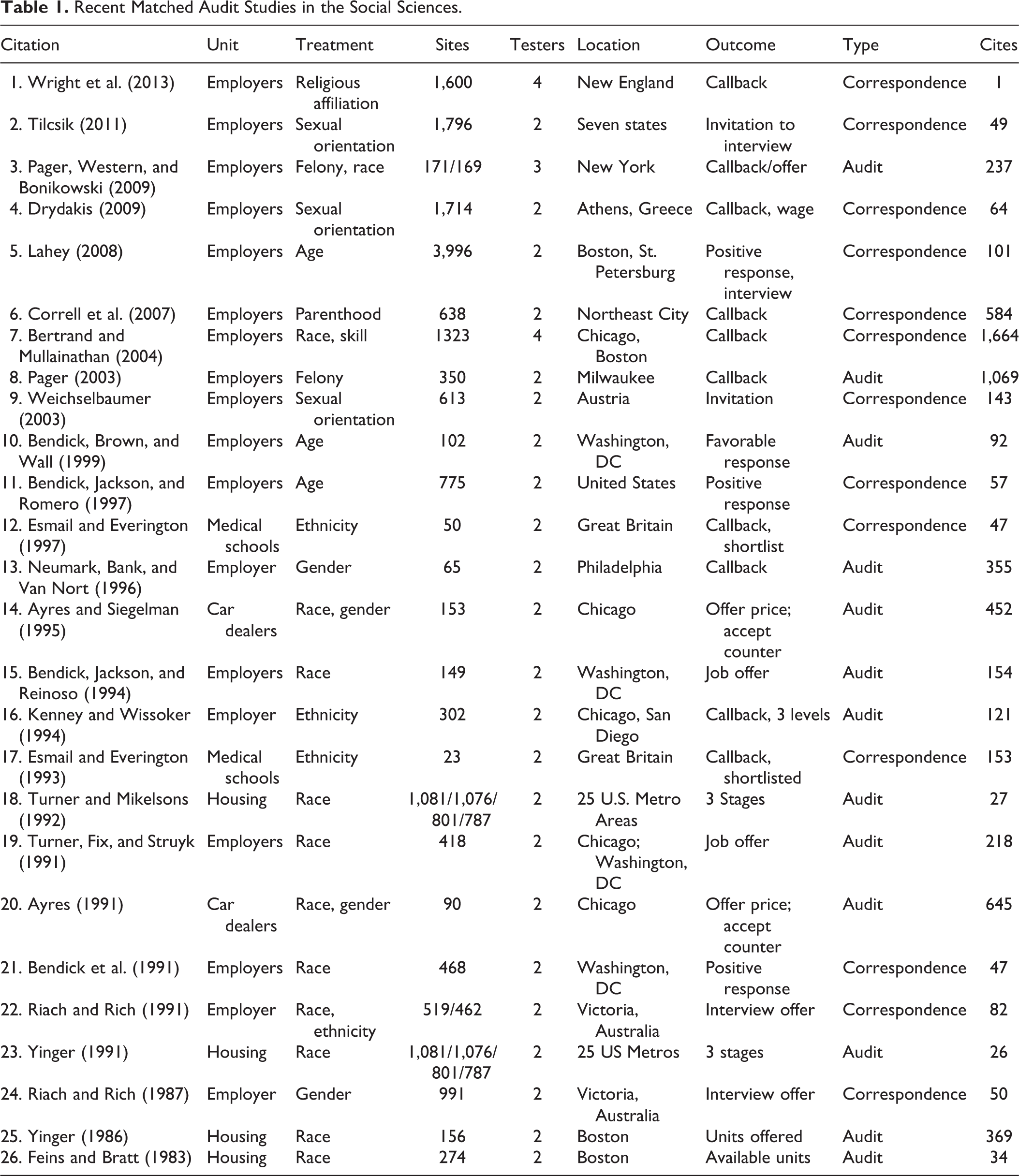
Three points are immediately apparent from the table. First, sample size varies greatly, as indicated by the number of sites. Some studies are based on fewer than 100 experimental units (Neumark, Bank, and Van Nort 1996), while others exceed 3,000 (Yinger 1991). Second, the treatments now being tested extend far beyond racial discrimination to include factors such as religious affiliation (Wright et al. 2013), sexual orientation (Tilcsik 2011), and parenthood status (Correll, Benard, and Paik 2007). Finally, without regard to discipline, almost all of these studies are extremely well cited. Based on Google Scholar citation data for August 2014, Bertrand and Mullainathan (2004) have been referenced over 1,600 times, while Pager (2003) has been cited over 1,000 times. Moreover, a preponderance of these studies are published in flagship journals, with some of them ranking among the most cited social science articles within the period since their publication.
Although the importance of audit studies is clearly reflected in their visibility and influence, the question of appropriate sample size has yet to be explored. There are at least four good reasons to do so. First, experimental audits have far greater capacity to reveal causal mechanisms than do alternatives such as covariate adjustment analysis of survey data through the process of randomization, which for audits is accomplished via random selection and matching (Pager 2007; Quillian 2006). These research endeavors are thus of great scientific and policy importance. In fact, randomized experiments are often considered the “gold standard” of research (e.g., Sherman et al. 1998). Further, audits are capable of uncovering dimensions of social phenomena, such as discrimination, that are difficult to study otherwise, as expressed behavior in surveys and interviews is demonstrably different from that of actual behavior in audits (Lageson, Vuolo, and Uggen 2014; Pager and Quillian 2005). Thus, maximizing the chance of detecting a significant effect in audit studies should take a central role in the design phase.
The remaining three reasons are closely related to cost, funding, and feasibility. Following second then, audit studies are both time and resource intensive (see Appendix in Pager 2007), particularly those utilizing in-person data collection rather than correspondence-based tests. Although the latter cost substantially less because no live testers must be paid, research personnel are still needed in both cases to conduct a range of labor-intensive tasks (such as sampling, random assignment, quality control, and tracking responses). When researchers overestimate the number of sites required to detect a practically and statistically significant effect, valuable resources are wasted, especially for in-person experiments. Third, in the absence of a reasonable guide to power calculations, researchers will err on the side of caution, exhausting resources that could otherwise be deployed to expand the study to additional treatments or outcomes (e.g., adding a Latino group to a proposed test of discrimination against African Americans relative to Whites, adding women to a proposed study of discrimination against those with criminal records, and expanding response categories in hiring to distinguish between an interview offer and a job offer). Thus, proper sample size calculations for both additional treatments and outcomes could increase the scientific yield of studies without incurring additional costs.
Both of these lead to the final important reason for sample size calculations: from the perspective of proposal reviewers and granting agencies, there are currently few standards to evaluate the appropriateness of the proposed sample size and budget in audit studies. Particularly in these times of scarce and declining funding, there are tremendous opportunity costs for either overfunding (in terms of other studies that are not funded) or underfunding (in terms of the funded audit’s capacity to advance knowledge). Demonstrating the ability for increased scientific yield and appropriately allocated resources will both improve research proposals and assist in accurately appraising them for funding. Given the costs in time, resources, and money and the related potential to expand a study, maximizing power through careful sample size calculations is paramount.
Although power calculations are important for all of these reasons, the issues of matching and nominal outcomes complicate their application in experimental audit studies. We begin by introducing the appropriate statistical test for these designs.
The Generalized Cochran-Mantel-Haenszel Test
With dichotomous experimental outcomes, as in the social science audit studies outlined previously, the choice of an appropriate statistical test is not as straightforward as it is for a continuous experimental response variable, for which the most appropriate statistical methods are variants of matched-pairs t-tests. Specifically, these experiments conform to a completely randomized block design (Pinheiro and Bates 2004), but with a nominal outcome in the case of an audit study. The block makes audit and correspondence studies unique relative to other field experimental designs, where each experimental unit only receives either a treatment or a control (e.g., the well-known field experiments testing mandatory arrest in police calls for spousal abuse; Berk et al. 1992; Sherman and Berk 1984). The block then is the experimental unit that is randomly selected, with each unit having repeated measures of both the treatment(s) and the control. To broadly apply the discussion that follows, we refer to the object whose response is being tested as the experimental unit, the dichotomous outcome coded 1 as an affirmative response, tester as the individual observations or cases presented to the experimental unit, treatment as the presence of the condition being tested, and control as the absence of the condition. For example, in the empirical example that follows for a dichotomous outcome with a single treatment, we tested whether employers (experimental unit) called back (affirmative response) either of two job applicants (testers), when one presented an arrest record (treatment) and the other presented a clean record (control).
We next describe the larger family of statistics to which audit studies conform. The appropriate statistical tests for matched experiments with nominal outcomes fall under a larger family of statistics known as generalized Cochran-Mantel-Haenszel (CMH) tests for O × R × S tables, where O = number of outcome response categories, R = number of repeated measures (i.e., treatments plus controls), and S = number of strata (Birch 1965; Landis, Heyman, and Koch 1978; Mantel and Byar 1978). 2 For a matched design, S = N; that is, a matched design is a generalized CMH test where each experimental unit is its own stratum (Agresti 2002:413–14, 458–59). 3 In determining sample size, it is this latter value that we seek to compute, as O and R are typically predetermined based on the research question. Table 2 summarizes the various tests in this family based on the values of O and R whose sample size selection we will discuss. As shown in the table, analyzing paired data with two repeated measures and a dichotomous outcome, the generalized CMH reduces to McNemar’s (1947) test. An example of such a design is the empirical example described previously. When there are multiple treatments and a dichotomous outcome, the statistic is known as Cochran’s Q (Cochran 1950). For example, a researcher could send testers of three racial categories to the same employers and measure whether each receives a callback. Finally, with two repeated measures and a nominal outcome with more than two categories, the Stuart–Maxwell test is appropriate (Stuart 1955). Although unexplored up to this point, a hypothetical example would include sending two testers of differing racial categories to the same employer and measuring three different responses, such as receiving no callback, receiving a callback for the position advertised, or receiving a callback for a lesser position (see, e.g., Pager, Western, and Bonikowski 2009). We will first address the more straightforward case of two repeated measures with a dichotomous outcome, which itself presents considerable sample size selection challenges, before addressing the case of more than two repeated measures or outcome categories.
Types of Generalized Cochran-Mantel-Haenszel Tests.
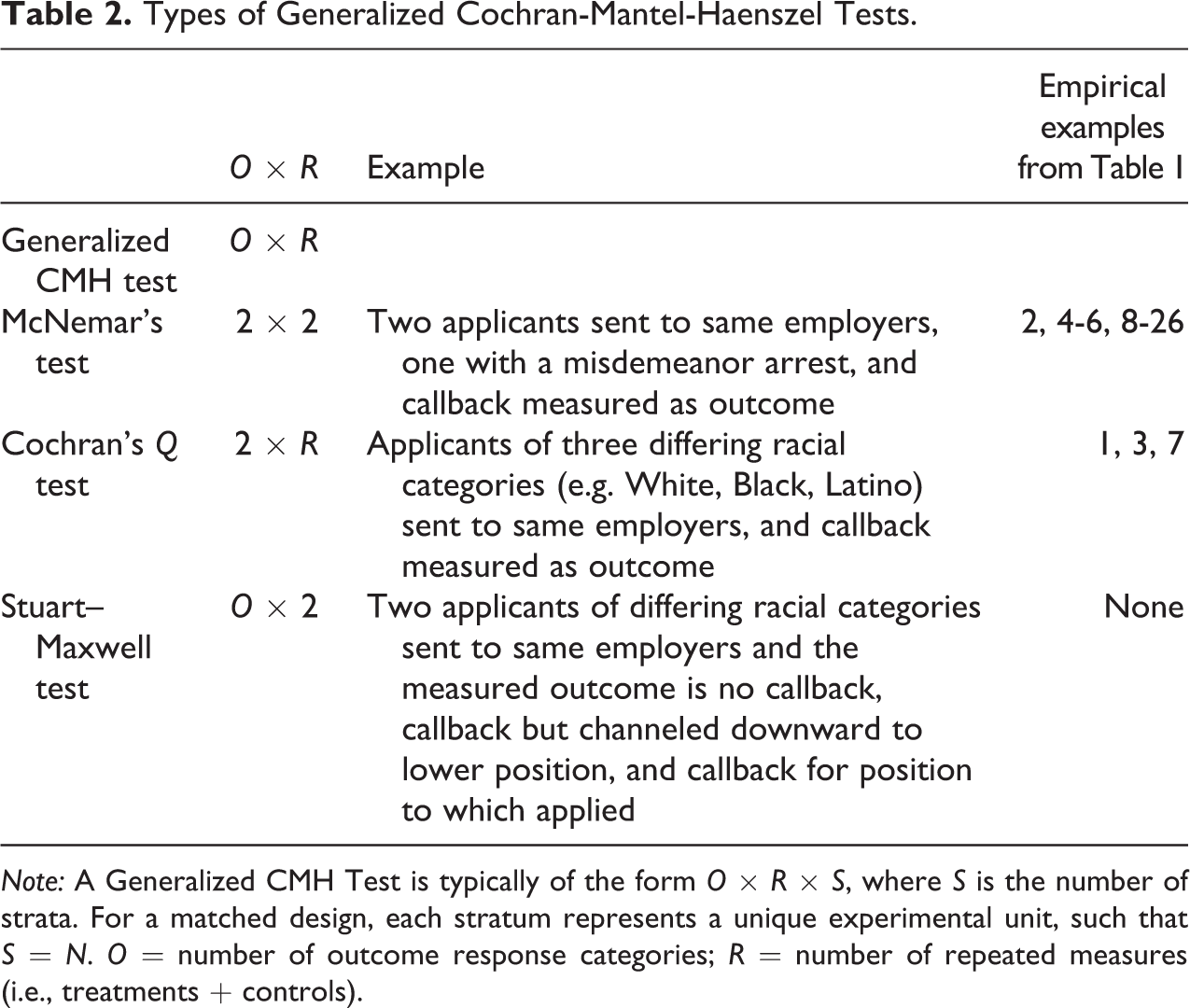
Note: A Generalized CMH Test is typically of the form O × R × S, where S is the number of strata. For a matched design, each stratum represents a unique experimental unit, such that S = N. O = number of outcome response categories; R = number of repeated measures (i.e., treatments + controls).
McNemar’s Test: One Treatment and a Dichotomous Outcome
Formulas and Notation for McNemar’s Test
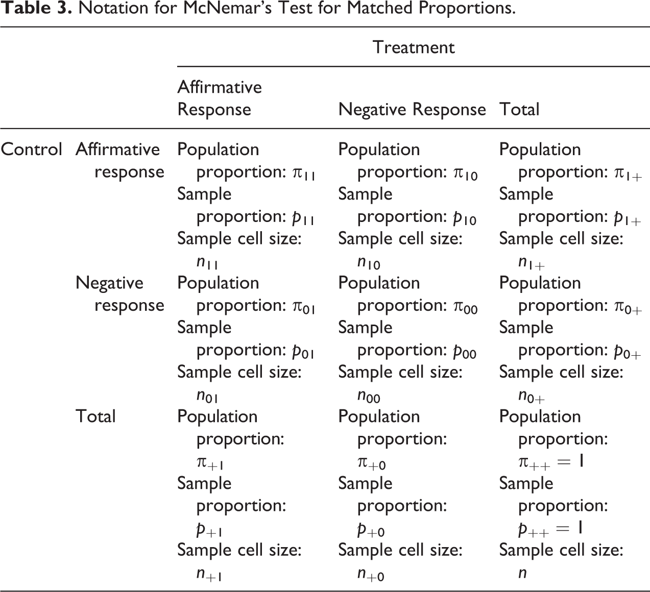
The simplest case of a 2 × 2 paired table conforms to McNemar’s test, with the notation
shown in Table 3 following
Agresti (2002:410–11). If we
consider the main treatment effect of interest in most of the articles outlined in Table 1 (see “Testers” column),
they conform to this table.
4
In Table 3, π
ab
denotes the population probability of outcome a for the first
tester and outcome b for the other tester for the same experimental unit
(i.e., different or discordant outcomes). nab
represents the count of the number of pairs in each cell, with
sample proportion equal to pab
= nab
/n. In what follows, we denote an affirmative response as 1 and
a negative response as 0 in the subscripts. The first subscript represents the outcome for
the control tester, while the second subscript represents the outcome for the treatment
tester for the same experimental unit. McNemar’s test assesses the hypothesis of marginal
homogeneity or H
0: π1+ = π+1. This is equivalent to testing equality
between the cells in which testers had different outcomes (i.e., H
0: π10 = π01), or that the difference between the two
discordant proportions is zero in the population. We can easily prove this result by

Notation for McNemar’s Test for Matched Proportions.
Thus, inserting the variance into the Wald ratio, the test statistic simplifies to the
following:
Note that the McNemar test statistic depends only on cases classified in different categories (i.e., the discordant cells) for the two matched observations. Of course, all cases contribute to inferences about how much π10 and π01 differ because the total proportion in the two concordant cells affects the total proportion in the two discordant cells, as they must add to 1. Yet, for this experimental design and test, the breakdown between the two concordant cells is irrelevant. In other words, the results are identical regardless of the split between the cells where both testers simultaneously receive affirmative or negative responses (i.e., only p 11 + p 00 is relevant, but not either term individually). This fact becomes important in power and sample size calculations, as two relationships determine the values: (1) the total discordant proportion (p 10 + p 01) relative to the total concordant proportion (p 11 + p 00) and (2) the relative proportion in the two discordant cells (p 10 and p 01).
Following Rosner
(2011:384–86), we provide the equations for power and sample size for McNemar’s
test. Let 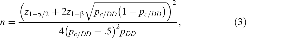
and the formula for the power for McNemar test with a set α, sample size
n, and Φ as the cumulative distribution function of the standard normal
distribution is as follows: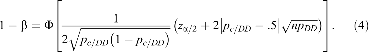
The results are symmetric, such that the same sample size and power emerge when the values of π10 and π01 are interchanged. For a one-sided hypothesis, α/2 is replaced by α.
All calculations were obtained with the statistical software program R (R Development Core Team 2006). We created functions for calculating power and sample size for McNemar’s test. Although some functions are available in the “TrialSize” package, we created a function with additional features. For example, our function allows for both one-sided and two-sided hypotheses. We also created a function that automatically produces a sample size table for a given α and β (as equivalent to Table 4) and power calculations for a given sample size (as equivalent to Table 5). In addition, functions are available for the sample size for the Stuart–Maxwell test and Cochran’s Q test. For the latter, this function represents the first of its kind, which is important given the increasing use of more than one treatment in audit studies. These functions are available on the first author’s website.
Sample Size Required for a Power of 0.80 for McNemar’s Test.
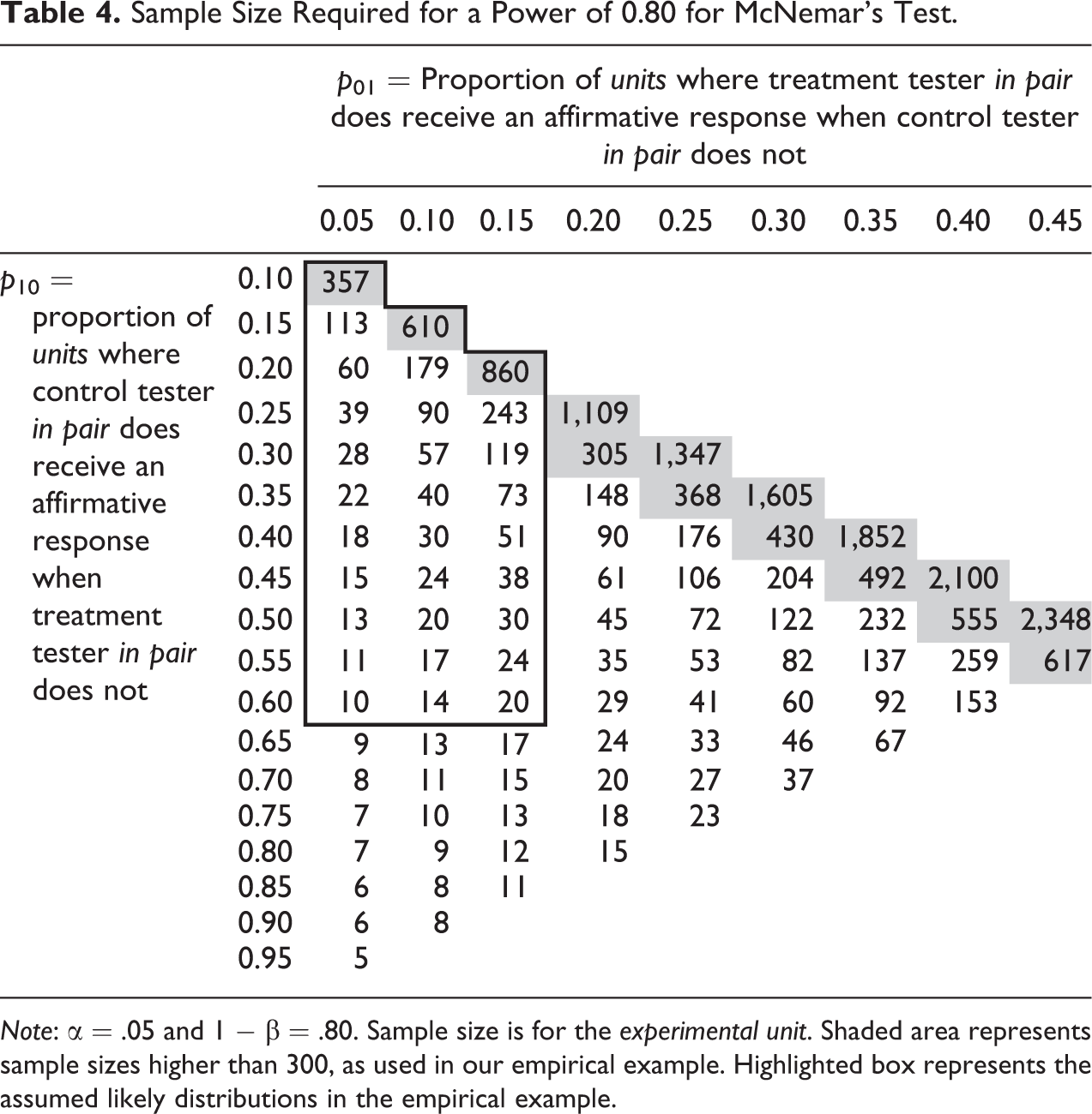
Note: α = .05 and 1 − β = .80. Sample size is for the experimental unit. Shaded area represents sample sizes higher than 300, as used in our empirical example. Highlighted box represents the assumed likely distributions in the empirical example.
Power for McNemar’s Test with Sample Size of 300.
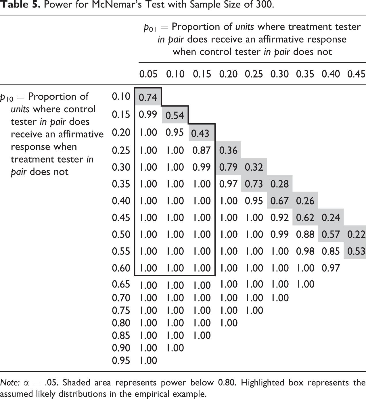
Note: α = .05. Shaded area represents power below 0.80. Highlighted box represents the assumed likely distributions in the empirical example.
Sample Size Calculations, Choices, and Challenges
Table 4 shows the sample sizes
that result from the one-sided versions of the formulas above with α = .05 and 1 − β =
.80. For McNemar’s test, we present the one-sided case because it is directly applicable
to our methods in the empirical example that follows, though the formulas, functions, and
calculations are easily extended and analogous to the two-sided case.
5
In what follows, we adopt terminology whereby the one-sided hypothesis favors
higher values in the cell in which the control receives affirmative responses and the
treatment does not (H
0: π10 > π01), though the symmetric nature of the
calculations allows for the reverse to be considered by simply swapping the notation
between treatment and control. In employment discrimination studies, higher values are
often anticipated in the cell in which only the control receives an affirmative response.
As noted, the results depend on the percentage in each of the discordant cells, though the
total concordant cells (regardless of the distribution across the two concordant cells)
will be determined by the proportions that fall into the discordant cells. Thus, the rows
of Table 4 represent the
proportion of all experimental units where the control tester received an affirmative
response when the treatment tester did not, or
By examining Table 4, we can compare required sample sizes for similar magnitude differences. For example, the very first entry in Table 4 where p 10 = 0.10 and p 01 = 0.05 has the lowest value of pDD , with pDD = 0.05 + 0.10 = 0.15 and pCC = 1 − 0.15 = 0.85. In the design phase, there is thus an assumption that for this five percentage point difference in the outcome, 85 percent of the cases fell into the concordant cells where neither or both tester received a callback. Only the control received an affirmative response 10 percent of the time and only the treatment received an affirmative response 5 percent of the time. The necessary sample size to detect this difference is 357. The cell for p 10 = 0.15 and p 01 = 0.10 also has a five percentage point difference in the outcome, but here pCC = 0.75 and the necessary sample size to detect this five percentage point difference is much larger at 610. Similarly, all cells following that first diagonal exhibit a five percentage point difference, but require very different sample sizes to maximize the chances to detect the same size effect. As shown in the table, power is lower as p 10 and p 01 simultaneously approach 0.5 (or that the sum equals 1). For example, consider two extreme cases. First, in the cell where p 10 = 0.55 and p 01 = 0.45, we have p CC = 0 (i.e., all the pairs were discordant) and the necessary sample size is 617. Second, in the cell where p 10 = 0.75 and p 01 = 0.25, we still have pCC = 0, but the necessary sample size is only 23 given the very large magnitude difference. 6
We use these examples to demonstrate the difficulty of considering only the magnitude difference when planning a matched field experiment with a dichotomous outcome. Instead, the proportion in the concordant cells and the breakdown in the respective discordant cells influence sample size choice. Researchers’ expectations of these quantities, together with the hypothesized effect size they would like to detect, must guide sample size selection. As will follow in our example and recommendations, we suggest that when designing a paired experiment with a dichotomous outcome, it is best to identify the realistic areas of Table 4 and choose a sample size that maximizes the chances of finding a significant effect for a given sample size across several possible outcome distributions. Both the concordant proportion and the amount in each discordant proportion are difficult to determine a priori. One would need information about how often either both or neither of the testers receives an affirmative response, and, for the discordant cells, how often the hypothetically unlikely case occurs when the treatment tester receives an affirmative response while the control tester does not. This challenge is best illustrated with an empirical example, to which we now turn.
Application to an Empirical Example
Despite the difficulties inherent in predicting concordance versus discordance and the separate discordant proportions in advance of a study, we can still calculate power for various sample sizes and show how this varies across these factors. We demonstrate this exercise with an empirical example (described in full in Uggen et al. 2014). In an audit study modeled after Pager (2003), we sent same-race pairs to 300 randomly selected establishments in the Twin Cities metropolitan area, with one applicant reporting no criminal history and the other reporting a misdemeanor arrest record. Four young male testers applied for entry-level jobs using fictitious identities. 7 All entry-level advertisements were selected, so long as they required no special skills or licenses, instructed applicants to apply in-person, and were located in the seven-county Twin Cities metropolitan area. Each week from August 2007 to June 2008, one tester in each pair was assigned to the treatment condition, that is, a single misdemeanor disorderly conduct arrest. Over the course of eight months, each pair submitted close to 300 applications at 150 job sites, with each tester assigned to the treatment condition for half of the audits. Our primary dependent variable was an employer “callback,” measured by an offer of employment or an invitation for a second interview (whether in-person or through e-mail or voicemail).
In selecting our sample size, we chose such that a reasonable difference could be detected across most of the distribution where realistic values of p 10 and p 01 fell, while staying within the confines of the available budget. This reasonable difference is typically between 5 to 10 percentage points. Here, we describe the calculations that led to this choice.
As described in the previous section, in the design phase of a matched field experiment, researchers must determine two numbers that are difficult to know a priori: the expected proportions in both discordant cells, as determined by the difference one wishes to detect, and the expected amount in the concordant cells. We viewed high values of p 01 as unlikely. That is, we assumed it would be rare for the otherwise equally qualified applicant with the arrest record to receive a callback when the applicant with a clean record did not. (Rather, we viewed concordance as much more likely: If the treatment tester received a callback, then the control was expected to as well). In one respect then, we used such likelihoods as anchors to determine the section of Table 4 into which our expectations fell. For the other unknown, we also viewed a low amount of total concordance as unlikely. That is, we assumed that there would be many employers who would call back both or neither tester (although irrelevant for power, we particularly viewed the latter as constituting many of the employers). Thus, we saw the outlined box in Table 4 as the area in which our study design was realistically positioned. Within this box, p 10 reaches a maximum of 0.60, while p 01 does not exceed 0.15. Depending on the distribution between concordant and discordant as well as the two discordant cells’ distance to 0.5, we have the power to detect an effect should it exist in the population at a magnitude difference of between 5 and 10 percentage points.
Put another way, within the confines of the resources available to us, we were comfortable with a low power to detect an effect where the percentage point difference in the discordant cells was only 5 to 10 percentage points. Once a sample size is selected, we can reverse the question and consider the exact magnitude difference that is detectable for different levels of concordance. As Table 5 demonstrates, considering the power across all the possible concordant and discordant combinations while restricting the sample size to 300, power is quite high when the magnitude difference exceeds five percentage points in our highlighted box. For example, with 300 employers and an assumption that p 01 = 0.05 (the first column of the highlighted box), the threshold where power 0.80 is crossed equates to a 5.55 percentage point difference (i.e., p 10 = 0.1055). If instead we are located in the last column of our highlighted box where p 01 = 0.15, we can detect an 8.9 percentage point difference (i.e., p 10 = 0.2390) with a power of 0.80.
We now discuss the observed results from our audit study (for a full discussion, see Uggen et al. 2014). Table 6 displays the distribution of callbacks. According to the marginal callback rate, testers with no misdemeanor arrest received a callback to 33.0 percent of their applications, while those with an arrest received a callback to 29.0 percent of their applications. These marginal proportions, however, do not take into account the result of the other tester in the pair at the same employer, which would lead to potentially erroneous conclusions if a χ2 test was conducted on this cross tabulation or a z-test of proportions (which assume independence). 8 In fact, Donner and Li (1990) showed that McNemar’s test is a function of a Pearson χ2 and a kappa statistic. The latter can be interpreted as the estimated correlation between members of a matched pair under the null, such that the relative magnitudes of the classical unmatched and matched χ2 statistics depend solely on the degree of resemblance within members of a matched pair (Donner and Li 1990:828; cf. Newcombe 1996).
Distribution of Callbacks by Criminal Record for Each Paired Audit and McNemar’s Test.
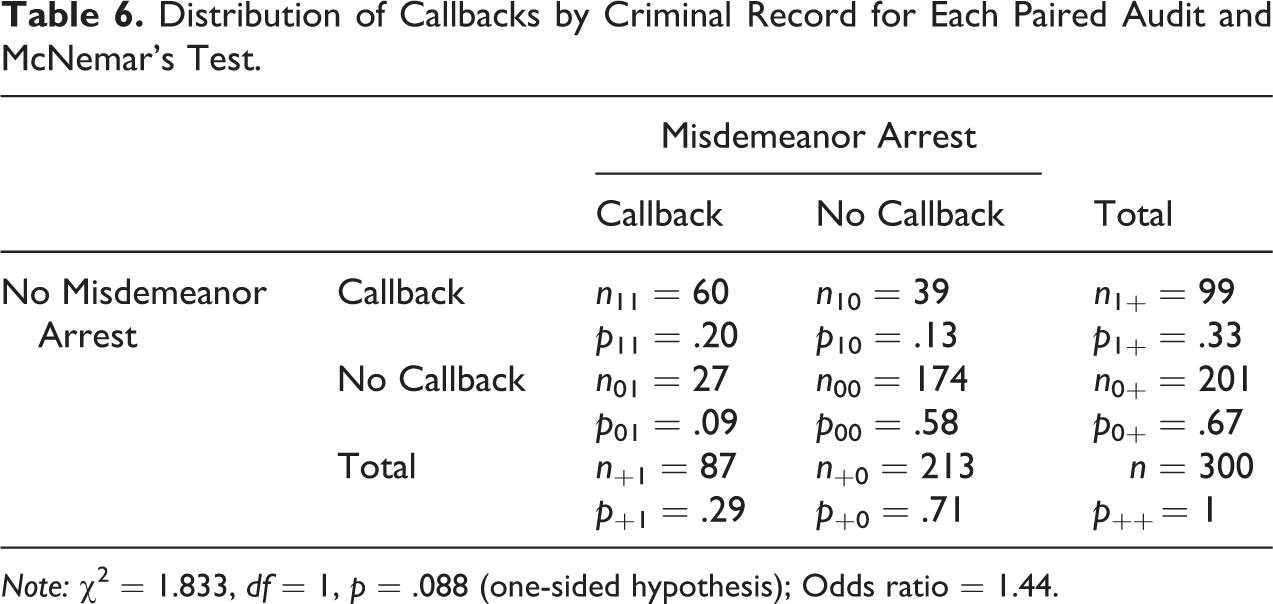
Note: χ2 = 1.833, df = 1, p = .088 (one-sided hypothesis); Odds ratio = 1.44.
Unfortunately, articles do not consistently report the pair-specific cross tabulations, which is the information future researchers need to use past studies as guides to calculating sample size and power. The marginal callback rate that is often given in matched audit studies prior to statistical modeling does not provide the needed pair-specific outcomes, which are shown in the pair-specific cross tabulation in Table 6. For example, while 33.0 percent of testers without an arrest and 29.0 percent of testers with an arrest received a callback, only 13.0 percent of the former received a callback when the latter did not and 9.0 percent of the latter received a callback when the former did not. If future researchers want to use past research as a starting point for sample size and power calculations, these pair-specific numbers are necessary information. Comparing our observed results with the expectations in our sample size analysis also reveals some of the difficulties in calculations for matched designs.
Given the observed concordance and relatively low percentage point difference in the discordant cells in our conducted study, the power to detect such a difference is relatively low, consistent with our a priori assumptions. 9 Compared to our assumptions, we observed a much higher proportion of concordance (pCC ) and proportion of employers where only the tester with the record received a callback (p 01) relative to the proportion of employers where only the tester without the record received a callback (p 10). In other words, we assumed that for such a high callback rate for the treatment tester only, the control tester only would receive a higher number of callbacks than was observed. Across the sample of 300 employers, pCC = 0.78, p 01 = 0.09, and p 10 = 0.13. Each of these numbers implies that we are near the very top of our outlined boxes in our tables. That is, even though they were otherwise comparable on all characteristics (and with the misdemeanor record rotated between the testers), the tester with the record received a callback when the tester without the record did not at a full 9 percent of the employers. Thus, we encourage researchers to prepare for this nonintuitive cell in their sample size calculations, which we clearly underestimated relative to p 01, as well as to collect covariates that might explain this anomaly, points to which we return in our recommendations.
Another important consideration is the degree of concordance. In addition to the observed discordance, the concordance of 78 percent was much higher than anticipated. The concordant cells are often difficult to determine beforehand. Although only their sum is relevant, understanding the context of each cell is necessary to make a realistic conclusion about the sum. For example, the 58 percent of the employers who called neither tester was highly dependent on local labor market conditions. Thus, even with information from a prior study, this cell, and thus the sum of the concordant cells, may be difficult to assign. In the cell in which both testers received a callback, constituting 20 percent of the sample, the amount is dependent on the relative “strength” of the treatment. Relatively “weak” treatments (here a misdemeanor arrest as opposed to Pager’s 2003 felony prison record) are correspondingly more likely to be overlooked. In such cases, we would expect high concordance in the affirmative cell, but would still have little reason to expect only the tester presenting the record to receive a callback.
As is typical for power curves, the relationship is not linear. As Table 4 shows, the sample size shrinks precipitously, as the magnitude of the percentage point difference in the two discordant cells increases and as this same difference extends farther from 0.5 (i.e., higher concordant percentages). Although power is most appropriately considered a design question, this result implies that even small changes in our observed data between these cells closer to our assumptions would have resulted in an acceptable power level. For example, if just 10 of the 60 employers who called back both testers instead called only the tester without the record, the power to detect the resultant difference would be 0.82. Similarly, if just 7 of the 27 employers in our unlikely cell who called back only the tester with the record had instead called back neither tester, the power to detect this difference would be 0.81. Thus, even though the power to detect the observed difference is low, small shifts in our observed data toward our a priori assumptions would have made the power more reasonable. This result emphasizes the need to consider a large range of possible outcome distributions when selecting sample sizes.
Stuart–Maxwell Test: More Than Two Outcome Categories
Although not yet considered in the social science literature, we could also easily envision scenarios in which there are still two paired testers, but the outcome has more than two response categories. This might arise, for example, if African American applicants are “channeled” to a lower position than the one advertised, while Whites are not (see, e.g., Pager, Western, and Bonikowski 2009). In such a scenario, both applicants would receive a positive response from employers, but we might want to know whether the type of response differs by race. Thus, there would be two testers but three outcomes: (1) callback for advertised position or higher, (2) callback but channeled downward, and (3) no callback. Not surprisingly, the challenges of sample size selection become greater as the number of outcome categories grows. Therefore, it is important to also consider sample size and power calculations for the case of these contingency tables.
As noted, the case of McNemar’s test generalized to more than two response categories is
known as a Stuart–Maxwell test (Stuart
1955; see also Agresti
2002:458–59).
10
This test still assesses the assumption of marginal homogeneity, H
0: π
i
+ = π
+i
, but instead does so simultaneously for all i, with
i = 1, 2, … , r response categories. This again amounts
to simultaneously testing the equality of all possible discordant combinations, or
H
0: π
ij
= π
ji
for all i, j = 1, … , r,
i ≠ j. Thus, r response categories and
r (r − 1)/2 null hypotheses are simultaneously tested.
More intuitively, this hypothesis tests whether the proportion for each possible combination
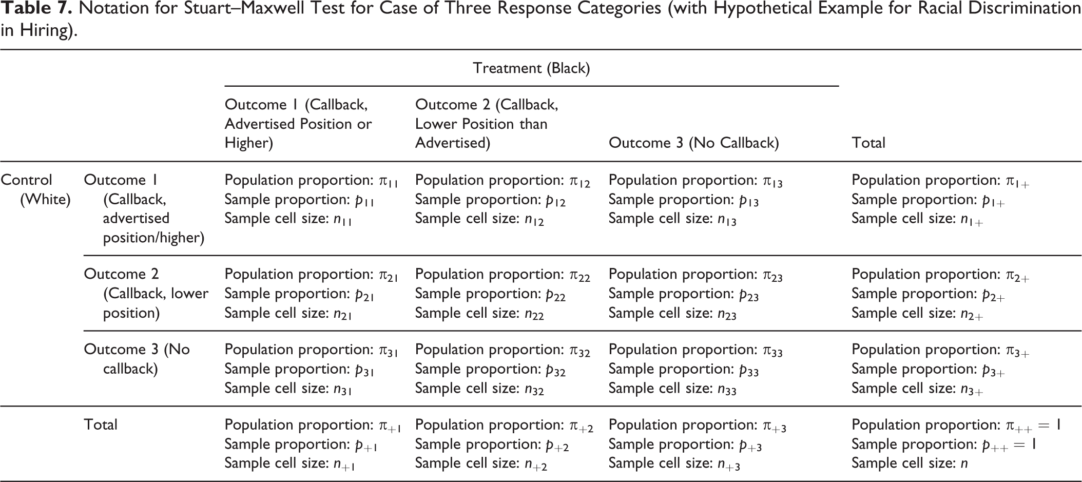
of outcomes is the same for the two treatments. Table 7 shows notation analogous to that presented
for McNemar’s test for the Stuart–Maxwell test for r = 3 outcome
categories, with an accompanying example following that given earlier. For
r response categories, the Stuart–Maxwell test statistic is:
Notation for Stuart–Maxwell Test for Case of Three Response Categories (with Hypothetical Example for Racial Discrimination in Hiring).
Based on the derivation of the exact test, Chow, Shao, and Wang (2003:154–55) present the
following sample size formula:
where λα,β is the noncentrality parameter from a noncentral χ2 distribution for a desired α and β and r degrees of freedom.
As with the case of two outcome categories, the determination of sample size, as well as the test itself, only uses information from the discordant cells. Again, this calculation amounts to having an estimate of the total proportion in the concordant cells and each of the discordant cells beforehand. We briefly demonstrate sample size calculations for the case of r = 3. Here, the r (r − 1)/2 = 3 null hypotheses being simultaneously tested are π12 = π21, π13 = π31, and π23 = π32. For the above-mentioned example, the null hypotheses would state that African Americans and Whites receive the same percentage for all three possible discordant comparisons. As in analysis of variance (ANOVA), we reject the null for the overall Stuart–Maxwell test when there is evidence against any of these null hypotheses. In the case of two outcomes, the required sample size grew as the difference between the discordant proportions decreased and as the sum of the discordant proportions simultaneously grew closer to 1. For two outcomes, this meant the discordant proportions simultaneously approached 0.5. For r outcomes, this implies that the discordant proportions simultaneously approach an even split, or 1/[r (r − 1)]. So for the case of three outcome categories, the highest sample size is required when the proportion in each discordant cell is close to 0.167. As the gap between the comparisons grows, a lower sample size is required. But this is offset by the total amount in the concordant cells. As is the case with two outcomes, the same two factors again determine sample size: the difference between the discordant cells and the total amount in the concordant cells. The difference here, of course, is in the former, where any given comparison can alter the sample size calculation.
For example, if we want to detect the same five percentage point difference in all the outcomes between the control and the treatment and assume in our distribution that all π ij = .13 and all π ji = .18 (and thus a total of 0.07 in the concordant cells), then we would need a sample size of 451 for α = .05 and 1 − β = .80. If, however, the five percentage point difference assumes all π ij = .05 and π ji = .10 (and thus a total of 0.55 in the concordant cells), the required sample size would be 219. Again, the required sample size to achieve the same power is not consistent for the same percentage point difference. In these examples, we assume the proportion in each of the discordant outcomes for the treatment and control are the same, respectively, but there is no reason to assume such.
To depict the required sample sizes for our example of three response categories, we chose several illustrative comparisons and graphed them in Figure 1. We take a graphical approach because reproducing a table similar to Table 4 for McNemar’s test is challenging since we can only show one π ij versus π ji comparison, while fixing the others at specific values. In other words, the sample size values in the table for one π ij versus π ji comparison differ depending on the proportions in the remaining discordant cell comparisons. In the figure, we concentrate on the π12 versus π21 comparison. In our example, these values represent the proportion of employers that call back the White or the Black tester, respectively, for the job advertised or higher (outcome 1), while the other tester receives a callback for a lower position (outcome 2). We vary the assumed proportion for the control group (π12, or the White tester receives the more favorable response) in the figure, while fixing its comparison to the treatment group (π21, or the Black tester receives the more favorable response) at 0.05, 0.15, and 0.25.
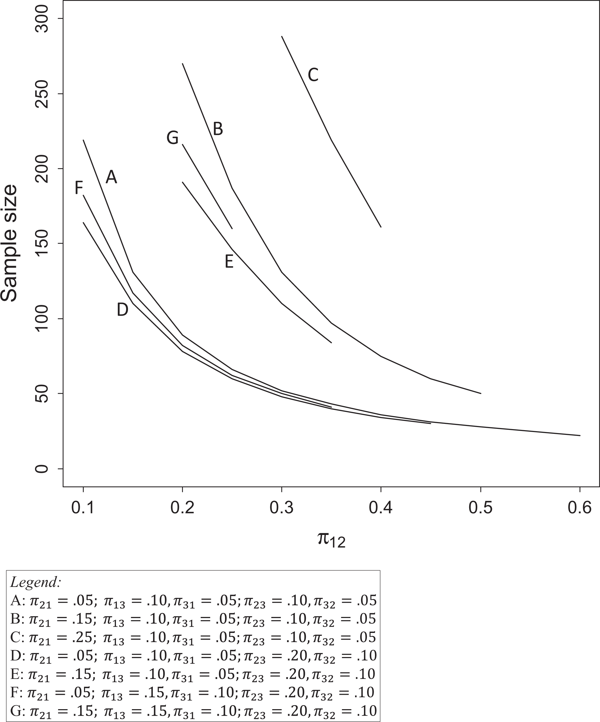
Required sample size for Stuart–Maxwell test. Note. α = .05 and 1 − β = .80.
Lines A, B, and C fix the other two outcome comparisons at 0.05 and 0.10 for the treatment and control, respectively. Reading left to right from the y-axis, each line begins with a five percentage point difference, yet the sample sizes differ because the total amount in the concordant cells decreases as π21 increases. At the beginning of line A, π12 = .10 and π21 = .05, replicating the previous example with a required sample size for power 0.8 of 219. At the beginning of line B, π12 = .15 and π21 = .20. With this decrease in the total concordant cells, the required sample size for this five percentage point comparison is 270. If we go further with line C where π12 = .25 and π21 = .30, the required sample size is 288. For each line, as we only vary π12, the required sample size decreases as the percentage point difference for the comparison under consideration increases across the x-axis.
The remaining lines then vary the other two comparisons. (Since the proportions must add to 1, the lines are of varying lengths.) The second comparison (π13 vs. π31) represents the proportion of employers where the White or Black tester, respectively, receives a callback for the advertised position or higher (outcome 1), while the other tester receives no callback (outcome 3). We keep the same five percentage point difference for lines D and E, while shifting to .15 and .10 for lines F and G. The third comparison (π23 vs. π32) represents the proportion of employers where the White or Black tester, respectively, receives a callback for a lower position than advertised (outcome 2), while the other tester receives no callback (outcome 3). Across lines D through G, there is a 10 percentage point difference (.20 vs. .10) for this comparison. With the larger difference for that comparison, these four lines are lower than lines A through C. For lines F and G, the second comparison is still a five percentage point difference, but results in a lower proportion in the concordant cells, and thus requires a higher sample size compared to lines D and E. The figure thus illustrates how the two challenges associated with a priori assumptions when calculating sample size also apply to more than two outcomes (i.e., the total amount in the concordant cells and the relative proportions in the discordant cells). Of course, the increased difficulty comes in assigning proportions to three discordant cell pairs. Although it is nontrivial to add an additional outcome, researchers may have good theoretical reasons to do so, such as the hypothetical example provided previously. Although there is increased difficulty in determining sample size, there may be relatively little cost, yet great scientific yield, associated with increasing the number of outcomes. By using the functions we provide, however, some of the difficulty in sample size determination is alleviated. We return to these points in our recommendations.
Cochran’s Q Test: More Than Two Repeated Measures
Although several of the audit studies reviewed earlier only use two testers per experimental unit, some have used three or more repeated observations. For example, Pager, Western, and Bonikowski (2009) sent White, Latino, and African American applicants to the same employer, and Bertrand and Mullainathan (2004) sent four applications to the same employer for each combination of White or African American of high and low qualifications. Sample size calculations for extending to more than two treatments are less straightforward than extending to more than two outcome categories. As mentioned previously, the case of McNemar’s test generalized to more than two repeated observations is known as Cochran’s Q statistic (Cochran 1950; see also Agresti 2002:458–59; Patil 1975; Wallenstein and Berger 1981). This test also assesses a version of marginal homogeneity, H 0: π1++ … + = π+1+ … + = … = π+++ … 1 for the m treatments (which is the number of subscripts). More intuitively, it tests whether the treatments have the same effect—whether the difference in the proportion of affirmative responses to each treatment is zero in the population. Note the differences between the case of r outcomes and m treatments. For the r outcomes, the Stuart–Maxwell test assesses whether a series of bivariate comparisons in an r × r table are all equal. For the m outcomes, Cochran’s Q simultaneously tests whether all the treatments in m 2 × 2 tables are equal.
We can again rewrite the hypotheses in terms of just the discordant cells. We use the
example of three treatments to illustrate. Unlike the case of additional outcome categories
where we can visualize the proportions in an r × r table
(see Table 7), when we add
additional treatment categories, we instead increase the dimensions of the table. In a
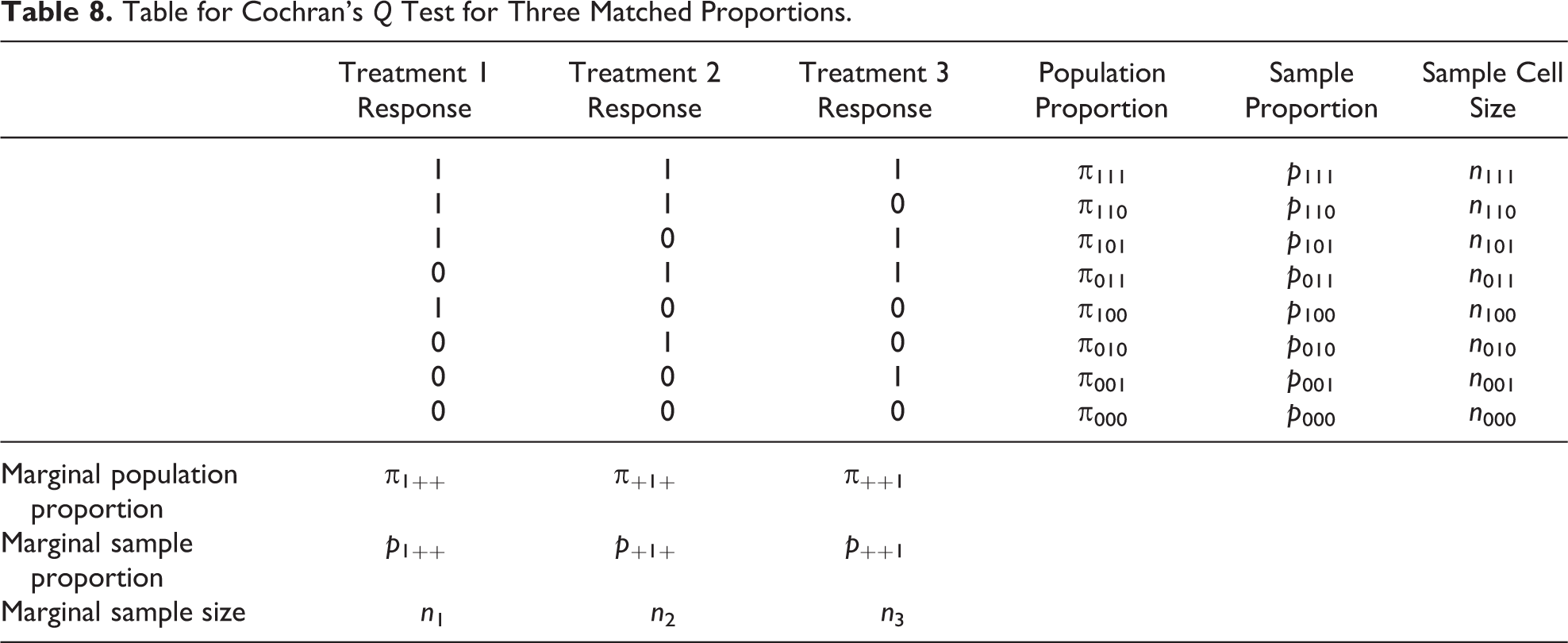
visual format suggested in Cochran’s
(1950) original article, Table
8 shows the notation for three treatments. Thus, the null hypothesis is
H
0: π1++ = π+1+ = π++1. When we rewrite the null
as a series of differences, we see again that the test only depends on discordant
cells: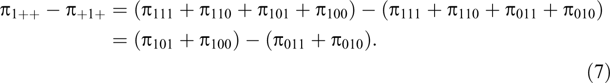
Table for Cochran’s Q Test for Three Matched Proportions.
Similarly,

Essentially, each difference removes the common occurrence of an affirmative response from the comparison, since the treatments are equally effective in that case.
For m treatments and Ai
representing the number of affirmative responses by experimental unit
i, i = 1, … , n, such that

where Q is distributed as
Calculating sample size for Cochran’s Q requires a unique approach. To our
knowledge, no one has attempted to explicitly state an exact formula or create a function to
calculate sample size for Cochran’s Q, due to the difficulty in inverting
the formula under the alternative hypothesis to solve for N. In light of
the relationship between Pearson’s χ2 statistic and Cochran’s Q
test, Donner and Li (1990) state
that sample size calculations can be computed by multiplying the required sample size for
the independent contingency table for each treatment (see Lachin 1977) by a kappa statistic κ
m
for intraclass correlation (Cohen 1960; Fleiss
1981; Scott 1955). Thus,
we provide a function that takes the sample size calculation for an independent
m × 2 table of the marginal proportions as given in Lachin (1977), which we denote
n⊥, and multiplies this value by a reexpressed version of the
weight proposed by Donner and Li
(1990:831), which we call wQ
:
where
and pj
represent the proportion of units with affirmative response value
j,
With regard to the weight, a kappa statistic measures interrater reliability. When it is less than zero, there is poor agreement. When it is between 0 and 1, it measures the degree of similarity. Thus, wQ = 1 − κ m assigns higher weights, and thus sample size, when the agreement is poor, which here implies higher discordance. The weight is smaller when the concordance is high. With more than two treatments, however, there are different degrees of concordance based on the number of affirmative responses within a given experimental unit (e.g., π111 is “more concordant” than π110, although the latter is “equally concordant” to π100 because the number of like responses is the same). Through the lead coefficient in the numerator, wQ thus weights more heavily those cells that are “more discordant,” which becomes especially relevant as the number of treatments grows. When the responses are “completely” concordant (i.e., either all or no affirmative responses), it is easy to see that those cases do not contribute to the numerator, as the lead coefficient is zero. Like the test statistic itself, however, knowledge of the proportion of experimental units with all affirmative responses is needed to calculate the denominator. Although technically one does not need the proportion for the cell where no testers receive an affirmative response, this cell will be predetermined since all other cells are required.
As with the previous two statistical tests, the weight results in a higher required sample size as both the total concordance decreases and the differences in the marginal proportions decrease. Demonstrating this numerically is more difficult than with either McNemar’s test or the Stuart–Maxwell test because there is no direct comparison between two proportions. As the null hypotheses show, each marginal comparison actually contains several discordant proportions. Further, each null contains overlapping proportions for cells where more than one affirmative response occurred. Unfortunately then, altering a given proportion can affect more than one null comparison, increasing the difficulty in considering a range of possible sample sizes. In fact, the researcher must provide all the proportions. In the case of three treatments, there are eight proportions, as demonstrated in Table 8. For four treatments, there are 16 proportions, which is shown in Online Appendix C. Thus, considering values required for sample size calculations quickly becomes onerous as m increases.
We provide a format for researchers calculating sample size for Cochran’s Q in Table 9. In this hypothetical example, we consider an audit of racial discrimination in hiring using White, Black, and Latino applicants. The statistical test is evaluating whether the marginal proportions are equivalent, given the clustering. In example 1, Whites received a callback in 44 percent of applications, Latinos in 23 percent of applications, and Blacks in 16 percent of applications. Simply computing a sample size for these numbers as independent, however, would ignore that each margin shares constituent proportions with the other treatments. Thus, above the marginal values, we provide the matched proportions that led to these marginal proportions, in which Whites are assumed to receive more callbacks, while Latinos and Blacks (either solely or together) receive fewer callbacks, and the proportion of concordance is 0.50. In this example, the required sample size is 103 for α = .50 and 1 − β = .80. In example 2, we consider a case with less of the overall proportion in the concordant cells at 0.30. Yet, we distribute that 0.20 decrease such that the marginals remain of the same distance from one another (within one percentage point due to rounding). Here, decreasing the amount of concordance results in a required sample size of 145. Thus, for an equivalent percentage point difference in the marginals, we again require differing sample sizes. In example 3, we keep the proportion of concordance the same as in example 1, but reduce the level of discrimination. Even with what amounts to very small shifts in the various discordant proportions, the required sample size increases to 372. Thus, shifts in both concordance and discordance again contribute to sample size, but here they are complicated by the fact that each marginal contains multiple constituent proportions.
Cochran’s Q Sample Size for Hypothetical Test of Racial Discrimination in Hiring.
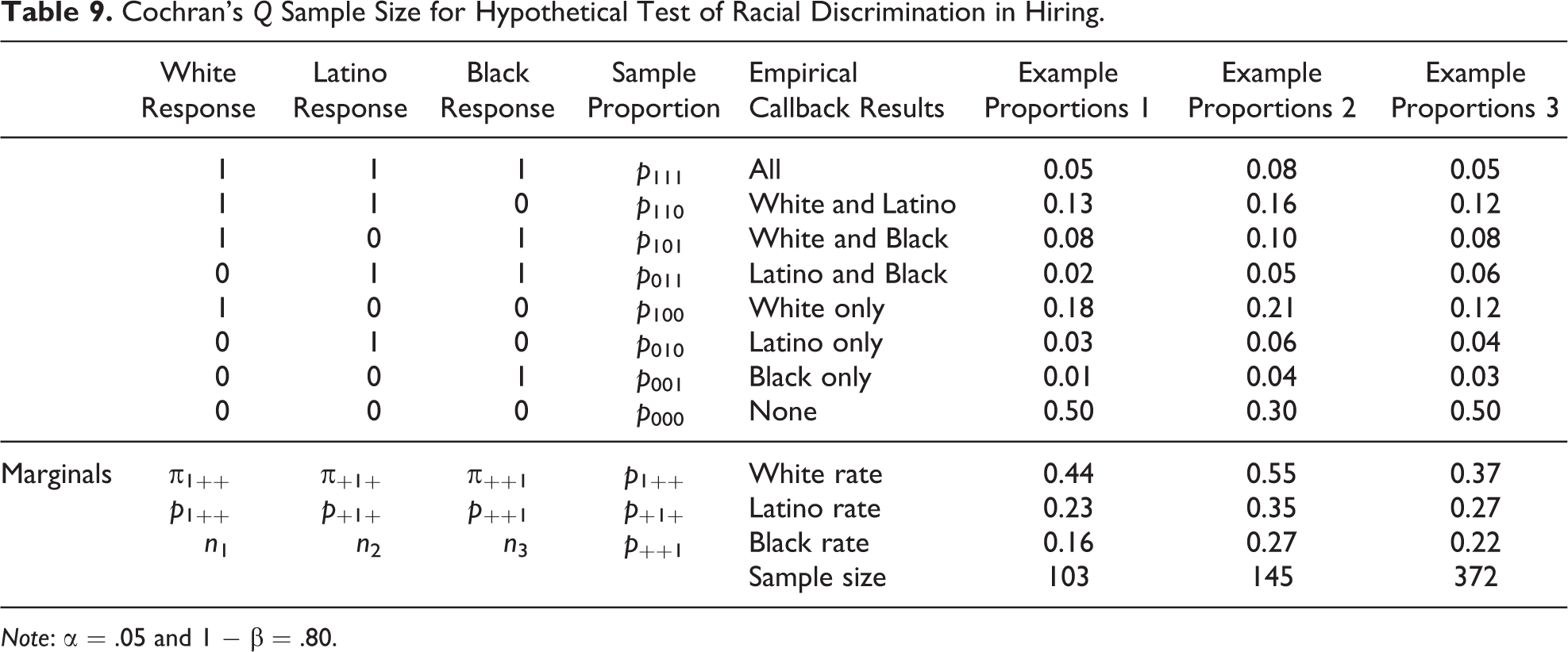
Note: α = .05 and 1 − β = .80.
Cautions for Extensions of the Method
In the social sciences, researchers also typically display linear models. For continuous outcomes, ANOVA and linear regression with only the treatment effect(s) in the model lead to the same results for power, sample size, and inferential conclusions. When data are clustered, fixed effects (FE) logit models with only the treatment(s) effects are analogous and lead to similar conclusions, although differing estimation procedures may produce slight differences in the bivariate test. In the case of equal exposure within experimental units to both the treatment and the control, as for audit studies, the bivariate tests are also equivalent to a random effects (RE) logit model with just the treatment effect as a predictor. Given this equivalency, the choice of RE or FE for the bivariate logit model is of little consequence, and the calculations here are easily extended to the generalized linear model with only the treatment effect included.
Typically, many articles employ an additional explanatory variable of interest (e.g., race in Pager 2003; gender in Correll et al. 2007). These variables, however, do not conform to the typical definition of a stratification variable within the generalized CMH framework, in which the experimental unit is contained within a mutually exclusive category of a confounding variable that cannot be randomly assigned (e.g., employers are not contained within race in Pager 2003 or within gender in Correll et al. 2007; cf. employers contained within states in Tilcsik 2011). Those variables also cannot be considered another treatment level because it was not varied within experimental units (cf. Bertrand and Mullainathan 2004; Pager, Western, and Bonikowski 2009). Thus, these examples are more akin to separate McNemar’s tests by the second variable of interest. By design, they cannot covary with the treatment, as no variation exists within employers on that measure (essentially constituting a covariate rather than a treatment, which is why we consider them as such in this discussion). Similarly, covariates collected during an audit would not constitute stratifying variables because they cannot be known beforehand. Nevertheless, these cases highlight the importance and utility of additional statistical modeling, which we consider further in the discussion section. We note here that, in such cases where additional covariates are included, RE logit models are likely the preferred choice, as several important covariates, including those listed in the studies previously, only vary across experimental units and thus are not estimable in the FE framework.
Although we might be interested in an additional stratifying variable as opposed to a covariate, such a test, along with its corresponding sample size formula, is not developed in the literature specifically for matched pairs. This would constitute a four-way table with O outcome response categories, R repeated measures, S = N strata for each experimental unit, and some other stratification variable to which each experimental unit would a priori belong (e.g., Tilcsik’s [2011] interest in the effect of state in an audit of employers’ hiring of gay men might conform to a four-way design). For multidimensional contingency tables, researchers usually turn to log-linear models for cell counts. For matched designs, however, this is not possible because the strata variable with N categories would have to be included, which would imply that every cell only contains either a 1 or a 0 (see Agresti 2002:233–34, 413–14, table 10.2), which would create problems in their estimation (Agresti 2002:391–98). Nonetheless, we encourage researchers to consider the question of sample size for such complex cases in the future.
Discussion and Recommendations
In this article, we demonstrated the difficulties in calculating sample size for a matched experimental audit. Researchers typically approach power and sample size from the perspective of magnitude differences. Yet, we show that for the matched audit design, phrasing the question in this manner is dependent on two factors. First, the total amount in the concordant cells contributes to power and sample size calculations. Second, the relative amount in the discordant cells requires a higher sample size as the difference between the cells decreases and the sum of the discordant cells approaches 1. These two factors result in a scenario in which, for a given power, different sample sizes are required for the same magnitude difference between the treatment and the control. We also show that these difficulties are greatly complicated by an increase in either the number of treatments or the number of outcome categories. Thus, we encourage researchers and reviewers to approach power and sample size for audit designs with a range of potential magnitude differences in mind.
Given the importance of audit studies to the social sciences, as discussed in our review, we do not intend to diminish their utility. Instead, carefully designed audit studies have the potential to identify causal mechanisms in ways generally not possible through survey research. Rather, our goal has been to gather the various statistical tests for audit designs and to explicate the challenges of sample size selection to facilitate the design and effectiveness of these approaches. We provide functions in R to assist researchers planning an audit study. In consideration of both the importance of these studies and our analytic results, we offer the following recommendations regarding sample size calculations for those considering a matched audit design.
Recommendation 1: Conduct a Pilot Study for Sample Size Calculation Purposes
Although several audit articles mention a pilot or testing period, these often are geared toward fine tuning the audit procedure itself (e.g., appropriate signaling of the treatment on resumes and training of live testers). Once such issues are resolved, we highly recommend an additional pilot for purposes of computing sample size. One of the advantages of each of the sample size formulas presented is that they only require the proportion in each discordant cell. When the pilot experimental units are randomly selected from the same population as the planned actual experiment, the proportions in each pilot cell should approximate those expected for the larger sample. Even a pilot with a small sample size can provide the necessary proportions, which will be far more helpful than uninformed sample size calculations or extrapolation based on the past studies (as discussed subsequently).
An accurate sample size calculation based on a pilot period is also extremely useful for both grantors and grantees in the funding application process. Granting agencies typically expect sample size calculations for primary data collection. A more informed sample size calculation, such as that based on a pilot study, would give granting agencies greater confidence that a proposed budget is appropriately allocated. Grantees who have conducted a pilot thus have the advantage of confidently demonstrating the minimum sample size (and corresponding budget) necessary to detect an experimental effect with an acceptable level of power.
Recommendation 2: Prepare for Several Different Concordant Sums
Of course, even pilot studies require some level of funding, potentially limiting this possibility. Another alternative is to use past studies, where available, to estimate the proportions beforehand. Whether using a pilot study or past studies, researchers should prepare for several different concordant sum possibilities, using the highest sample size. The concordant cells represent cases in which the testers receive the same outcome at the same experimental unit (e.g., both or neither job applicant receives a callback). The sum of these cells might be highly dependent on both location and time. For example, in an audit of hiring decisions, the ability of both or neither tester to receive an affirmative response from employers depends on prevailing economic conditions. Thus, past studies conducted in a different geographic location can only provide a rough estimate of the total concordant proportion, as both the strength of the local economy and the types of jobs available will differ across localities. Even estimates drawn from the same geographic location are likely to change, as the onset of recessions or shifts in sector-specific labor demand could alter the total cases where both or neither tester is called back. Moreover, such changes can also occur between the pilot study and the eventual granting of funds. For all of these reasons, researchers should consider a range of potential concordant sums, informed by contextual similarities and differences. For example, researchers might weight the results of past studies by industry to produce a distribution similar to the local economy that is being tested.
Recommendation 3: Prepare for Several Different Discordant Differences
Choosing the proportion in the discordant cells also presents challenges. Researchers must look beyond treatment/control differences, since sample size requirements are quite different for the same magnitude difference in the discordant cells (as shown on any left–right diagonal in Table 4). Our hypotheses typically assume that the experimental unit will prefer the control to the treatment when given an otherwise equal choice, such that it would be rare for the experimental unit to respond affirmatively to only the treatment. It may thus be hard to imagine why researchers must prepare for high values for the case where the treatment receives an affirmative response, while the control does not (π01). Yet, even in our empirical example, we used theory to prepare for this possibility. Theories of statistical discrimination posit that employers use race to draw “quick and dirty” assumptions about group differences in productivity and other characteristics, particularly when they lack detailed information about applicants (Arrow 1973; Bielby and Baron 1986; Braddock and McPartland 1987; Moss and Tilly 1996; Phelps 1972; Tomaskovic-Devey and Skaggs 1999). Thus, if employers assume applicants, particularly African Americans males, harbor a serious criminal record, disclosing an arrest might actually alleviate concerns based on statistical discrimination, causing the employer to favor the applicant with the arrest. We still viewed this as an overall less likely occurrence in our sample size calculations, but accounted for up to a 15 percent callback rate where the arrest treatment would receive a callback when the control did not.
In general, the weaker or “milder” the treatment, the more researchers might expect higher values in that cell. Although we had theoretical reasons to believe employers might only call our treatment tester, other similar studies might have no reason to assign high proportions to that cell in sample size calculations. For example, with Pager’s (2003) treatment of a felony prison record, there is little reason to believe that divulging such a record would put an applicant in a favorable position over an equally qualified control applicant. In contrast, our own misdemeanor arrest treatment was considerably milder. Similarly, in Correll et al.’s (2007) test of parenthood, while we might expect nonparents only to receive a callback more of the time, we would not expect parenthood to be a wholly disqualifying characteristic. Thus, where the treatment is not wholly disqualifying, additional sources of variation that are not easily foreseeable or accountable might affect this cell. For example, an employer might possibly prefer parents (Correll et al. 2007), racial minorities (Pager, Western, and Bonikowski 2009), or those of a stigmatized religious identity (Wright et al. 2013), or the honesty associated with divulging a criminal record (Uggen et al. 2014).
Finally, we caution that additional sources of variation may occur in field experiments compared to laboratory experiments. Some of the cases in which only the treatment received a callback might be due to other nonrandom factors. For example, jobseekers who make direct contact are much more likely to be called back by employers, who may wish to provide a “second chance” to an otherwise promising applicant (Pager, Western, and Sugie 2009:206). If only the applicant with an arrest record is successful in making contact with the hiring authority, this may result in a callback only to the treatment. In a bivariate test such as those presented here, this additional source of variation is not addressed. Although we emphasize the importance of collecting important covariates in audit studies, we note that a properly randomized study should remove covariation between the treatment and the covariates that are subject to the randomization process. Although the covariates can still have significant and sizable effects on the outcome, they should not affect the magnitude of the coefficient and standard error, and hence significance, of the treatment effect. For example, of the 18 covariates in our audit study, only 1 (contact) affected the treatment’s coefficient and standard error to any discernable degree. 11 Thus, covariates are less a hindrance to power calculations in the experimental context, though they may be relevant to sample size if they affect the proportion in the discordant cells. Regardless of whether covariation exists between a covariate and the treatment, covariates can still covary with the outcome, and thus a multivariate framework still proves informative, as is presented in most sociological audit studies and discussed previously.
For many of the same reasons expressed concerning the sum of the concordant cells (e.g., labor market conditions), it is also difficult to determine how often the control will receive a callback when the treatment does not (π10). For each of these reasons, as in our empirical example, we suggest the consideration of a range of possible discordant combinations.
Recommendation 4: Report Results at the Experimental Unit Level
In the absence of a pilot study, we recommended using past studies for the assumed proportions, a common practice in sample size and power analyses. Unfortunately, many empirical articles do not present results in a paired format such as those in Table 6 (see Riach and Rich 2002 for a summary of economics articles in this format), but rather only present the marginals. Such an omission does not imply any statistical limitations of past studies, but rather implies the absence of a uniform standard for presentation. This is understandable, given the novelty of audit studies within sociology, as well as possible trade-offs between presentation and replicability. For the sake of future designs, however, we highly encourage authors to present the results in the paired format, utilizing the tests presented previously. Future researchers can then apply those values as an estimate for their proportions, and consider an appropriate range around them. By referencing multiple studies on similar topics, those designing audits can best calibrate that range. For example, in terms of audit studies testing criminal records, a future researcher might consider our empirical example on a misdemeanor arrest and Pager’s (2003) study on a felony conviction with time served as the minimum and maximum proportions they should consider. Armed with this information, more informed sample size decisions can be made. If no research has been conducted for the specific treatment or experimental unit under consideration, a pilot study may be more imperative.
Recommendation 5: Consider a Nonmatched Design
Finally, where cost is a major consideration, we encourage authors to consider a nonmatched experimental design. This would involve only sending one randomly selected tester to each experimental unit. In his influential critique of field experiments, Heckman (1998) argues exactly such a case, stating that the use of matched pairs is not necessarily preferable to sending randomly assigned testers to different job sites. Even when only one tester is sent to each experimental unit, the randomization process, here achieved through random allocation of the units to treatment and control rather than matching and random selection in the case of an audit, should ensure no systematic bias in the assignment of the treatment (Cox 1958). Substantively, the matched approach is not necessary unless one wishes to account for within-employer effects (e.g., by including random experimental-unit intercepts to account for concordance; see Agresti 2002:410–11, 467–68, 493–501). Of course, researchers may very well have such an interest in within-employer effects.
Despite yielding results with true experimental rigor, the relevant question here is whether there is a sample size advantage to one approach or the other. As described previously, Donner and Li (1990) showed that the independent Pearson’s χ2 test is related to the matched tests presented via a weight that measures intraclass correlation. This simple connection shows that lower sample sizes are required for matched tests when there is a greater expected degree of concordance (as was expected and occurred in our audit). Conversely, lower sample sizes are required for independent tests where there is a greater expected degree of discordance. 12 This result makes perfect sense: When there is no effect of the experimental unit, it is irrelevant whether one sends testers to the same unit. The implication for sample size is straightforward. When researchers expect great concordance within experimental units, a matched design would economize funds. When researchers expect a high degree of discordance, an independent design would be more cost effective, though one should still consider substantive interests in the effect of the experimental unit.
Conclusion
Experimental audit studies represent a powerful and flexible tool for drawing causal inferences about social processes. In all such studies, the power to detect a certain magnitude difference between the groups represents a key design consideration. Unfortunately, the paired nature of the data complicates efforts to compute a priori power calculations. This article has presented sample size and power calculations from our own empirical study, then offered formulas and examples for cases involving more than two treatments (Cochran’s Q test) and nominal outcomes (Stuart–Maxwell test). Beyond gathering these tests and explicating the challenges of sample size selection, we offer both concrete recommendations and the pertinent functions in R for estimating the appropriate size of future audit studies.
Supplemental Material
Supplemental Material, SMR570066_Suppl - Statistical Power in Experimental Audit Studies: Cautions and Calculations for Matched Tests With Nominal Outcomes
Supplemental Material, SMR570066_Suppl for Statistical Power in Experimental Audit Studies: Cautions and Calculations for Matched Tests With Nominal Outcomes by Mike Vuolo, Christopher Uggen and Sarah Lageson in Sociological Methods & Research
Footnotes
Authors’ Note
Acknowledgments
We are grateful to Zack Almquist and Sarah Mustillo for feedback on previous versions and to Lindsay Blahnik and Emily Harris for editorial assistance.
Declaration of Conflicting Interests
The author(s) declared no potential conflicts of interest with respect to the research, authorship, and/or publication of this article.
Funding
The author(s) disclosed receipt of the following financial support for the research, authorship, and/or publication of this article: The illustrative empirical data used in this article come from a study conducted in partnership with the Council on Crime and Justice and supported by the JEHT Foundation and the National Institute of Justice (grant number 2007-IJ-CX-0042). Uggen is additionally supported by a Robert Wood Johnson Health Investigator Award.
Notes
References
Supplementary Material
Please find the following supplemental material available below.
For Open Access articles published under a Creative Commons License, all supplemental material carries the same license as the article it is associated with.
For non-Open Access articles published, all supplemental material carries a non-exclusive license, and permission requests for re-use of supplemental material or any part of supplemental material shall be sent directly to the copyright owner as specified in the copyright notice associated with the article.