Assessing Discrimination in Correspondence Studies

Abstract

Correspondence studies are popular tools for assessing discrimination against minorities, for example, in the labor market. Typically, two fake Curriculum Vitae (CVs) are sent to multiple job openings. The CVs are equivalent except for a mark identifying the disadvantaged. While it is straightforward to establish discrimination from minorities’ lower response rates, it is often unclear what its source may be. Discrimination may result as much from employers’ aversion toward a minority, as from perceptions that members have lower or more dispersed abilities that are unstandardizable in a CV. We refine existing methodologies to propose a wider-scope method capable of disentangling these three sources of discrimination and establish its face validity applying it to a correspondence study aimed at assessing labor market discrimination against ex-convicts in a local market.

Keywords

audit studies correspondence studies taste discrimination statistical discrimination

Introduction

Audit studies are increasingly popular tools for assessing discrimination in employment (Bertrand and Mullainathan 2004; Pager 2003), housing decisions (Ewens, Tomlin, and Wang 2014), credit approvals (Dymski 2006), or consumer market transactions (Rich 2014). Typically, two demands (for a job, rental, credit, or product) are sent to a random sample of decision makers from fake applicants. Applicants’ merits are matched in everything, except their having or not a trait which may trigger the discriminatory practices that the experimenter aims to observe from decision makers. This trait is generally a mark/stigma signaling membership into a socially disadvantaged group—a minority, thereafter¹—such as women (Correll, Benard, and Paik 2007), an ethnic group (Booth, Leigh, and Varganova 2012; Pager 2003), or ex-convicts (Uggen et al. 2014). If decisions on the applications are significantly less favorable for minorities, discrimination is established.

The main difficulty in audit studies is not to find discrimination but to identify its various sources: from an aversion toward minorities—taste discrimination (Becker 1971)—to rational assessments about differences between minority and majority members in typical productivities—first-moment statistical discrimination—or in the variability of such productivities within groups—second-moment statistical discrimination (Heckman 1998; Heckman and Siegelman 1993; Neumark 2012).

While there have been some proposed solutions to distinguish taste from first-moment statistical discrimination—see, for example, Altonji and Perriet (2001), Lahey (2008), or Ewens, Tomlin, and Wang (2014)—and these two from second-moment statistical discrimination (Neumark 2012), to this date, a comprehensive approach combining them into a single method does not exist. The main contribution of this article is to propose such a method, one that allows estimating the three forms of discrimination provided some (testable) assumptions hold. We demonstrate its validity for the simplest form of an audit study—a correspondence study in which the outcome is to be or not to be selected for further screening—and for discrimination in the labor market.

This article is organized as follows. In the first part, we follow Heckman and Siegelman (1993), Heckman (1998), and Neumark (2012) to formalize the problems for separating the three forms of discrimination. In the second part, we review the existing solutions to these problems and propose our own. In the third part of this article, we show method’s usefulness by applying it to data from a correspondence study aimed at detecting discrimination against ex-convicts in a local labor market. Method’s strengths and weaknesses are discussed in the final section.

Taste Discrimination

Taste discrimination is typically defined as resulting from prejudice—a response expressing animus or aversion against an out-group that is not based on reason but on emotion (Lang and Lehman 2012).

Aversion is just one among the possible factors accounting for employers’ decisions to select a candidate for further screening. Heckman and Siegelman (1993) and Heckman (1998) proposed a probabilistic model of employers’ decision-making in which their selection decisions depend not only on prejudicial assessments of candidate’s appeal to employers but also on objective evaluations of candidate’s potential productivity. These evaluations are partly based on qualifications that can be standardized in a CV—on “observables.” They also depend on error-prone guesses about candidates’ unstandardizable qualifications—“unobservables”—based on clues rooted in experience.

More formally, let employer’s decision Y to select a candidate for a job interview depend on an underlying continuous variable Y* capturing candidate’s appeal to employers.² This appeal varies according to candidate’s productivity P, such that Y*(P). Candidates will be selected (y = 1), if their appeal equals or exceeds a minimum cutoff level c set by the employer (if Y* ≥ c). Let candidate’s productivity, in turn, depend on a set of candidate’s observable (X ₁) and unobservable ( ${\tilde{X}}_{2}$ ) qualifications and on firm’s F characteristics, such that $P (X_{1}, {\tilde{X}}_{2}, F)$ . Thus:

Y (Y^{*} (P (X_{1}, {\tilde{X}}_{2}, F))) = 1 if Y^{*} \geq c, and Y = 0 otherwise.

Correspondence studies hypothesize that candidates’ appeal depends both on their productivities (P) and on group membership (G). Minorities are less appealing and less likely to be selected than other candidates. Thus, under the alternative hypothesis:

Y (Y^{*} (P (X_{1}, {\tilde{X}}_{2}, F), G)) .

If we assume, for simplicity, that Y* is linear on P and G and that candidates’ productivity-related qualifications are uncorrelated with group membership $[Cov (P, G) = 0]$ , we can rewrite $Y^{*}$ in equation (1a) as:

Y^{*} = P + γ G .

If minority candidates are coded as 1 ( $g = 1$ ) and the other candidates as 0 ( $g = 0$ ), the expectation is that $γ$ will be negative when averaged across jobs and that the cutoff applied to minorities will be higher than that applied to the advantaged, due to employers’ aversion toward the former. Hence:

Y = 1 if P + γ G \geq c \equiv if P \geq c - γ G, and Y = 0 otherwise.

In sum, employers who discriminate minorities because they distaste them apply two cutoffs: $c$ for the majority and $c - γ$ for the minority.³ $γ$ is both a measure of the discrimination faced by minorities and the extra productivity they need to display to have the same appeal to employers as nonminorities.

Heckman and Siegelman (1993) argued against interpreting differences in minorities and nonminorities’ appeal to employers in correspondence studies as unequivocally capturing taste discrimination, due to undesired selection effects that cannot be effectively controlled with matching. Matching guarantees that the paired candidates demanding a job are equivalent on observables, except for the mark signaling membership into the minority. However, nothing guarantees that employers perceive the pair as having similar unobservables. Perceptions about the distributions of unobservables across groups, rather than aversion, may lead employers to discriminate against minorities. These perceptions may be about group differences in the mean levels or the dispersion of unobservables. The former lead to first-moment statistical discrimination; the latter, to second-moment statistical discrimination.

First-moment Statistical Discrimination

“First-moment statistical discrimination” (Neumark 2012) is typically portrayed as stemming from rational assessments of in- and out-groups’ stereotypical qualifications, as derived from experience (Levitt 2004). One first manifestation is when employers perceive the mean of the unobservables in the minority to differ from nonminorities’.

As assumed above and demonstrated by Heckman (1998), to estimate $γ$ without bias, a key assumption rarely spelled out in correspondence studies must hold—group membership and productivity must be independent $(P ⊥ G)$ . This holds for candidates’ $X_{1}$ observables, which experimenters match across groups, but might not hold for productivity-linked ${\tilde{X}}_{2}$ characteristics unobserved to experimenters but acted upon by employers. Two reasons explain it.

Suppose, for simplicity, that as in Heckman (1998), candidates’ productivities—on which employers base their selection decisions—are a linear function of, first, individuals’ $X_{1}$ observables and second, of their ${\tilde{X}}_{2}$ unobservables.

P = X_{1} + {\tilde{X}}_{2} .

We place a tilde above ${\tilde{X}}_{2}$ , the set of unobservables, to indicate that they pertain to all members of a group. Employers do not know candidates’ personal characteristics if omitted from the CVs. Any unobserved characteristic attributed to them must come from preconceptions about group members’ average productivity and typical dispersions.

In a correspondence study, experimenters fix candidates’ observables in the CVs, generally at similar levels across job offers, as they are not interested in estimating the effect of $X_{1}$ observables on productivity, but in establishing differences in selection rates between groups. By making observables equivalent across groups, experimenters ensure they are independent of group membership.

Let the relationship between productivity and candidates’ characteristics be deterministic⁴ regarding $X_{1}$ but probabilistic regarding ${\tilde{X}}_{2}$ . When employers are randomly selected for a correspondence study, their perceptions about candidates’ unobservables can be seen as defining the sampling distribution of candidates’ unobserved productivities. Let assume that employers’ perceptions of the productivities derived from candidates’ ${\tilde{X}}_{2}$ unobservables are normally distributed around the mean $μ_{{\tilde{X}}_{2}}$ corresponding to productivity level $p_{b}$ —where the subscript b stands for “baseline”—, with a variance of $σ_{{\tilde{X}}_{2}}^{2}$ .

{\tilde{X}}_{2} \sim N (μ_{{\tilde{X}}_{2}}, σ_{{\tilde{X}}_{2}}^{2}) .

Put differently, the productivities corresponding to candidates’ ${\tilde{X}}_{2}$ unobservables can be decomposed into a constant $p_{b}$ capturing employers’ perceptions of candidates’ average productivity associated with unobservables and an idiosyncratic error $∊_{i}$ expressing the typical error in such perceptions. Hence, the prediction equation for P derived from equation (4) above is:

P_{i} = p_{b} + X_{1} + ∊_{i},

where $p_{b} = E (P | {\tilde{X}}_{2}, X_{1} = 0) = E ({\tilde{X}}_{2}) = μ_{{\tilde{X}}_{2}}$ .

Let’s assume that employers perceive the means of the normal distributions of unobservable-related productivities to be the same for minorities and nonminorities, that is, that $E ({\tilde{X}}_{2}^{0}) = E ({\tilde{X}}_{2}^{1})$ (superscripts 0 and 1 stand, respectively, for nonminorities and minorities because like observables, unobservables are also independent of group membership $({\tilde{X}}_{2} ⊥ G)$ . If the assumption held and taste discrimination was the reason behind minorities’ lower selection rates, the prediction equation (2) for the underlying variable regulating selection probabilities could be rewritten as:

Y_{i}^{*} = p_{b} + X_{1} + γ' G + ∊_{i} .

However, if employers thought that minorities have lower (or higher) average productivities linked to unobservables than other candidates $(E ({\tilde{X}}_{2}^{1}) < E ({\tilde{X}}_{2}^{0}))$ , $γ'$ would capture, at least partly, employers’ beliefs about these group differences in average productivities (hence the prime superscript). This can be formalized as:

{\tilde{X}}_{2_{i}} = p_{b} + ∊_{i} = p_{b} + δ G + τ_{i},

where $E (τ_{i}) = 0$ and $δ$ equals the difference between minority and majority candidates in their appeal to employers because of their differences in unobservables.⁵

One possibility not contemplated in Heckman’s (1998) formalization of first-moment statistical discrimination is that employers may believe that the contribution of unobservables to productivity is different in each group.⁶ For example, they might think that hiring minorities may affect negatively the productivities of others workers who hold prejudices against them—see Ewens et al. (2014) for a similar formalization. These beliefs about the different contribution of unobservables’ to groups’ productivities may be important in shaping employers’ assessments of their different productivities. If these beliefs exist, then:

{\tilde{X}}_{2_{i}} = p_{b} + ∊_{i} = p_{b} + δ G + λ G + τ_{i},

where $λ$ equals the difference between minorities and nonminorities in the effect of unobservables on productivities.

Correspondingly, a candidate’s score on the underlying scale of appeal to employers will be:

Y_{i}^{*} = p_{b} + X_{1} + δ G + λ G + γ G + τ_{i} = p_{b} + X_{1} + (γ + δ + λ) G + τ_{i} .

If equation (10) holds, $γ'$ in equation (7), which supposedly estimated employers’ lower sympathy toward minorities, was biased because it included employers’ perceived differences ( $δ$ and $λ$ ) in minorities’ productivities relative to nonminorities $(γ' = γ + δ + λ)$ .

Second-moment Statistical Discrimination

A second problem in correspondence studies is experimenters’ implicit assumption that the variance in employers’ perceptions of candidates’ unobservables is the same among nonminorities and minorities

Var ({\tilde{X}}_{2}^{0}) = Var ({\tilde{X}}_{2}^{1}) .

However, employers may perceive that minorities differ more (or less) among themselves in unobservables than nonminorities. For example, experimenters may feel more uncertain about candidates’ unobservables when they belong to groups they know less. As argued by Heckman (1998), if employers perceived groups’ distributions of unobservables as being normally distributed but having different variances, their perceptions would result in different callback probabilities for each group, even if they applied the same selection cutoff to both and thought that both have the same average levels of unobservables (i.e., even if there was neither taste not first-moment statistical discrimination).⁷

When groups’ variances differ, it is difficult to predict which group will experience a lower callback probability, for this will depend on whether employers’ selection cutoff is below or above the mean of candidates’ unobservables, and on which group has higher variance. Our problem is how to distinguish this second-moment statistical form of discrimination from the other types.

Suppose that employers exert taste discrimination against minorities but not first-moment statistical discrimination. Further suppose that, as assumed in a typical correspondence study, $Var ({\tilde{X}}_{2}^{0}) = Var ({\tilde{X}}_{2}^{1})$ . Then, combining expressions (1) and (6) above, a candidate’s callback probability could be written as in a standard probit model:

Pr (Y = 1) = Pr (Y^{*} > c | X_{1}, {\tilde{X}}_{2}, G) = Pr (p_{b} + X_{1} + γ G + ∊_{i} > c) = Pr (∊_{i} > c - (p_{b} + X_{1} + γ G)) .

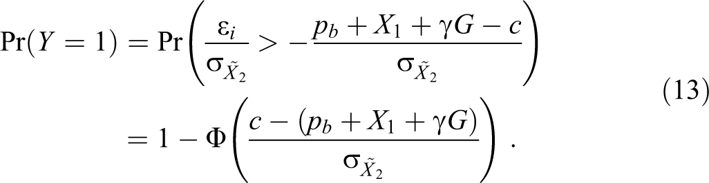
To identify the probit coefficients, they must be expressed in units of standard deviation of, in our case, the random variable ${\tilde{X}}_{2}$ capturing candidates’ unobservables:

Pr (Y = 1) = Pr (\frac{∊_{i}}{σ_{{\tilde{X}}_{2}}} > - \frac{p_{b} + X_{1} + γ G - c}{σ_{{\tilde{X}}_{2}}}) = 1 - Φ (\frac{c - (p_{b} + X_{1} + γ G)}{σ_{{\tilde{X}}_{2}}}) .

where $Φ$ is the standard normal cumulative density function.

In probit models, we cannot know the real variance of the underlying variable $Y^{*}$ and instead fix it to 1 to identify the model (Greene 2010). Hence, to solve equation (13), we standardize ${\tilde{X}}_{2}$ , setting $σ_{{\tilde{X}}_{2}} = 1$ , and, for simplicity, also $p_{b} = μ_{{\tilde{X}}_{2}} = 0$ :

Pr (Y = 1) = 1 - Φ (c - (X_{1} + γ G)) .

If $Var ({\tilde{X}}_{2}^{0}) = Var ({\tilde{X}}_{2}^{1}),$ callback probabilities will equal $1 - Φ (c - X_{1})$ when g = 0 (nonminority), and $1 - Φ (c - X_{1} - γ)$ when g = 1 (minority). Since $c - X_{1} - γ$ is higher than $c - X_{1}$ (remember that $γ$ will be negative if there is taste discrimination against minorities), nonminorities’ selection probability will also be higher than minorities’. If there is no taste discrimination, $γ = 0$ , and the two probabilities will be the same.

In contrast, suppose that employers perceive that the variance of candidates’ unobservables differs in the two groups $(Var ({\tilde{X}}_{2}^{0}) \neq Var ({\tilde{X}}_{2}^{1}))$ . Heckman (1998) shows that selection probabilities would then generally differ for each. To see this, specify equation (13) above for each group. Because the denominators defining groups’ variances differ, so do callback probabilities:

[1 - Φ (\frac{c - (p_{b} + X_{1})}{σ_{{\tilde{X}}_{2}}^{0}})] \neq [1 - Φ (\frac{c - (p_{b} + X_{1} + γ)}{σ_{{\tilde{X}}_{2}}^{1}})],

except if:

c - (p_{b} + X_{1}) = 0 and γ = 0,

15a

or if

γ = (1 - \frac{σ_{{\tilde{X}}_{2}}^{1}}{σ_{{\tilde{X}}_{2}}^{0}}) \cdot (c - (p_{b} + X_{1})) .

15b

Equation ( 15b) results from algebraically finding the value of $γ$ for which $(c - (p_{b} + X_{1} + γ)) / σ_{{\tilde{X}}_{2}}^{1}$ equals $(c - (p_{b} + X_{1})) / σ_{{\tilde{X}}_{2}}^{0}$ . It expresses how much higher or smaller minorities’ scores in $Y^{*}$ are relative to nonminorities due to their belonging to a group with higher or lower variance and the bias in estimating $γ$ (taste discrimination) when wrongly assuming variance equality.

Neumark (2012) proposed an equivalent formalization of the problem by making unobservables’ variances a function of group membership in a heteroscedastic probit model:

σ_{{\tilde{X}}_{2}}^{2} = {(e^{k + ω G})}^{2},

with $σ_{{\tilde{X}}_{2}}^{0} = e^{k}$ , and $σ_{{\tilde{X}}_{2}}^{1} = e^{k + ω}$ .

The callback probability expressed in equation (13) could then be reexpressed as:

Pr (Y = 1) = 1 - Φ (\frac{c - (X_{1} + p_{b} + γ G)}{e^{k + ω G}}) .

Standardizing equation (17) in relation to nonminorities’ parameters, that is, setting the mean $p_{b} = 0$ and the standard deviation $σ_{{\tilde{X}}_{2}}^{0} = e^{k} = 1$ (so that $ω = 0$ ), expression (15) could be rewritten as:

[1 - Φ (c - X_{1})] \neq [1 - Φ (\frac{c - (X_{1} + γ)}{e^{ω}})] .

Like equation (15) above, expression (18) states that callback probabilities differ for minorities and nonminorities, unless:

c - X_{1} = 0 and γ = 0,

18a

or:

γ = (1 - e^{ω}) \cdot (c - X_{1}) .

18b

Except for the normalizing assumption $p_{b} = 0$ , equation (18b) is equivalent to equation (15b), since $e^{ω} = σ_{{\tilde{X}}_{2}}^{1} / σ_{{\tilde{X}}_{2}}^{0}$ (Neumark 2012). Both express the bias in $γ$ when ignoring differences in groups’ standard deviations. Its magnitude and direction depends on (1) how large minorities’ standard deviation is relative to nonminorities’ (on the coefficient $ω$ defining the ratio $e^{ω}$ of groups’ standard deviations in equation [18b]) and (2) how far the level of observables set by the experimenter is relative to employers’ cutoff, as expressed in $c - X_{1}$ in equation (18b).

Distinguishing First-moment Statistical Discrimination from Taste Discrimination

The solutions applied in the literature to distinguish first-moment statistical discrimination from taste discrimination take into account their typical definitions—see Guryan and Charles (2013) and Neumark (2016) for recent reviews of this work. Here, we focus only on solutions using correspondence studies, but there have been other innovative approaches to separate statistical from taste discrimination that rely on lab experiments or a combination of field, lab experiments, and surveys (Anderson and Haupert 1999; Castillo and Petrie 2010; Fershtman and Gneezy 2001; Lahey and Oxley 2016; Levitt 2004; List 2004; Masclet, Peterle, and Larribeau 2012; Zussman 2013). The basic intuition behind these solutions, regardless of the methodology they employ, is that if taste discrimination is based on emotion and statistical discrimination rests on reason, only the latter could generate changes in employers’ selection decisions when candidates’ personal merits are experimentally manipulated, signaling that employers act rationally and react to the new information they receive.

As shown previously, in correspondence studies in which candidates are matched on observables, first-moment statistical discrimination ensues when employers perceive that groups differ in average levels of ${\tilde{X}}_{2}$ unobservables, or if they think that the same unobservables contribute differently to productivity in each group, as expressed in coefficients $δ$ and $λ$ in equation (9) presented above.

To estimate $δ + λ$ , the experimenter could add variables that are generally omitted in a CV (thus belonging to vector ${\tilde{X}}_{2}$ ) and calculate their effects on employers’ group preferences, holding constant minority and nonminority members’ observables through matching, randomization, or by hiding information on observables (Ahmed, Andersson, and Hammarstedt 2010; Bosch, Angeles Carnero, and Farré 2010; Carlsson and Eriksson 2017; Drydakis 2014; Ewens et al. 2014; Kaas and Manger 2012). Alternatively, and more economically, she could fix nonminorities’ scores on ${\tilde{X}}_{2}$ (e.g., at their mean), manipulate experimentally minorities’ scores on the same variables, and observe how much $δ + λ$ change as a consequence, as in gender discrimination studies that assign typically masculine traits to some female candidates to assess their probability of being selected compared to an average woman (Keinert-Kisin, Hatzinger, and Köszegi 2012; Weichselbaumer 2004). More formally:

δ + λ = {\bar{P}}^{1} - {\bar{P}}^{0} = {\bar{Y}}^{*, 1} - {\bar{Y}}^{*, 0} = η {\tilde{X}}_{2}^{1},

where the superscripts 1 and 0 stand, respectively, for the minority and the nonminority.

In expression (19), $η$ expresses how much the groups’ differences in productivities, and the corresponding differences in groups’ appeal to employers, change as minorities’ levels of unobservables are modified experimentally. It is a measure of how much employers allow minorities to compensate any group deficit/surplus with higher/lower personal unobservables and, hence, a measure of how much their discriminatory practice is grounded on perceptions about group differences in productivities.⁸ If $η = 0$ , $δ + λ$ will also be 0, and $γ'$ in equation (7) will equal $γ$ in equation (10), thus reflecting the constant penalty that minorities face due to employers’ aversion toward them. If $η \neq 0$ , first-moment discrimination is at place.⁹

The drawbacks of testing for $η = 0$ are that it calls for more complicated and costly designs requiring the creation of multiple candidates’ profiles with difficult to standardize traits. To avoid detection of the experiment, the tester may opt for randomizing the allocation of single applicants to different employers, rather than sending many fake CVs to the same employer, and to compare applicants’ rates of response across, rather than within employers (Lahey 2008). While useful, this strategy may be difficult to implement in some contexts, as when job search engines require applicants to register online before they can apply to a job. An alternative is to reduce the number of applicants’ profiles and send them to the same employer, but this will increase the probability of omitting relevant unobservables (Neumark 2016; Yinger 1998). If employers saw minorities and nonminorities as differing in these omitted characteristics, the tests devised to evaluate the presence of statistical discrimination might yield false negative results.¹⁰

Our recommendation is to vary minorities’ levels of observables, under the premise that deficits/surpluses in productivities linked to unobservables can be offset with higher/lower observables (we show how to test this premise below). This solution respects Heckman’s assumption that observables and unobservables are uncorrelated (that $X_{1} ⊥ {\tilde{X}}_{2}$ ) and instead assumes that at some level of $X_{1}$ and ${\tilde{X}}_{2}$ , they are exchangeable and substitutable because they will have the same effect on productivities and hence also on groups’ differences in productivities:

δ + λ = η {\tilde{X}}_{2}^{1} = φ ′ X_{1}^{1} .

However, adding variation in minorities’ $X_{1}$ observables will unmatch minorities and nonminorities’ levels of observables, making it impossible to tell, for example, if an equalization in the probability of being selected after raising minorities’ observables captures the additional qualifications needed to overcome taste discrimination (the higher cutoff placed on minorities) or the substitution mechanisms between unobservables and observables characterizing first-moment statistical discrimination. In other words, insofar as $X_{1}$ and $G$ are correlated, $φ'$ may also capture taste discrimination and be biased (hence the prime superscript).

Introducing variation in observables also in the majority group can control for differences between minority and majority members in observables. The experimenter could, for example, set two (or more) levels of observables for candidates applying to each job, sending more than two applications to each opening, and distinguish minority and majority members in each set—for precedents of multiple applications, see Bertrand and Mullainathan (2004), Booth, Leigh, and Varganova (2012), or Ewens et al. (2014). This means adding a coefficient $β$ to equation (10) above and estimating the impact of $X_{1}$ observables on the underlying variable $Y^{*}$ measuring candidates’ appeal to employers:

Y_{i}^{*} = p_{b} + β X_{1} + (δ + λ) G + γ G + τ_{i} .

Adding the same variation in $X_{1}$ for both groups raises yet another problem, as it makes it impossible to generate the differences between minorities and nonminorities’ productivities needed to assess employers’ reactions. Only if the added variation in observables affected differently groups’ appeal to the employers and their selection probabilities, it might be possible to use this interaction effect to assess first-moment statistical discrimination. Ewens et al. (2014)—see also Lahey (2008) and Ahmed, Andersson, and Hammarstedt (2010)—argue that this interaction ought to be expected when there is statistical discrimination, but they ground their expectation on the presence of differences in the variances of groups’ unobservables—that is, on the presence of second-moment statistical discrimination—a scenario that we contemplate in the next section.

In contrast, we argue that an interaction effect between the level of observables and minority membership should also be expected in the absence of second-moment statistical discrimination, provided that employers select for further screening all (or the first n) candidates who pass a single productivity cutoff, regardless of by how much they exceed it.¹¹ There is evidence that this selection model is widespread, especially in the first phase of multistage selection processes, and that it helps minorities to overcome deficits in some qualifications with surpluses in others (De Corte, Lievens, and Sackett 2007; Finch, Edwards, and Wallace 2009; Sackett et al. 2001).

If the cutoff can be passed with different bundles of observables and unobservables because what matters to employers is that the selected candidates certify meeting an acceptable threshold of productivity, not how they reach it, then any perceived group differences in productivities would manifest in an interaction effect between the level of observables and group membership. The reason for this interaction effect is the censoring of candidates’ productivities when they exceed the level (c) of the cutoff required to be selected. This censoring makes employers assign the same potential productivity to all candidates who pass the cutoff—the one needed to pass it. It makes the difference in candidates’ observables induced experimentally by the tester larger than the difference in candidates’ productivities actually considered by the employer when selecting candidates $((X_{1,High} - X_{1, Low}) > (P_{High} - P_{Low}))$ . This difference in differences is magnified when candidates have higher unobservables, since they will reach the cutoff sooner, all the more so, the more $(X_{1, High} + {\tilde{X}}_{2}) > c$ . It manifests in smaller returns to observables (smaller probabilities of selection) for candidates with higher unobservables—typically, nonminorities. Hence, the differences in candidates’ appeal to employers produced by minorities and majority’s differences in unobservables can be estimated by varying experimentally candidates’ levels of observables. This can be formalized by eliminating the prime symbol for $φ$ and the superscript for $X_{1}^{1}$ in equation (20):

δ + λ = η {\tilde{X}}_{2}^{1} = φ X_{1},

where $φ = η ({\tilde{X}}_{2}^{1} / X_{1})$ , that is, the very same differences in candidates’ appeal that were induced in equation (19) by altering the level of unobservables of the minority group, which is now expressed in terms of observables. Substituting $φ X_{1}$ for $δ + λ$ in the prediction equation clarifies that $φ$ is the interaction effect between $X_{1}$ and $G$ capturing the selection adjustments that employers make as differences in minority and majority members’ observables are made to vary experimentally, due to their perception that groups differ in unobservables.

Y_{i}^{*} = p_{b} + β X_{1} + φ X_{1} G + γ G + τ_{i} .

As in the case of $η$ , $φ$ can be zero, positive, or negative. If $φ = 0$ , there is no first-moment statistical discrimination. If $φ < 0$ , employers believe that group differences in productivities linked to unobservables decrease as minorities’ observables increase. Altonji and Perriet (2001) interpreted the wage corrections in favor of minority candidates with longer than average career histories as evidence that employers allow minorities to compensate deficits in unobservables with higher observables, and of first-moment statistical discrimination. If $φ > 0$ , employers believe that differences in productivities linked to unobservables become larger when minorities’ observables increase. This could be because employers consider some low qualifications to increase productivity. For example, in some businesses, employers may favor nonempathetic workers who have no scruples for closing ethically dubious sales (DeLiema, Yon, and Wilber 2016). Alternatively, employers may discriminate more markedly against minorities with high qualifications because they consider such qualifications to be improper of a low-status group and a threat to the nonminority’s higher status (Phillips, Rothbard, and Dumas 2009; Rudman et al. 2012). In both cases, employers’ adjustments would be based on rational estimates of majority and minority’s expected or prescribed productivities, rather than on negative feelings or prejudices against minorities, thus providing a valid test of first-moment statistical discrimination (Lahey 2008).

Equation ( 23) is the basis for calculating the penalty, in selection probabilities, that employers’ inflict on (non)minorities for each less unit of observables, if their deficits in unobservables are measured in these units. This adjustment can be obtained by calculating the partial effect or change in probability associated with $φ$ in expression (23) and by using the Delta method to derive standard errors (Norton, Wang, and Ai 2004). These standard errors must be clustered within jobs, to allow for autocorrelation in employers’ responses to the fake applications.

To calculate the difference in the partial effect of belonging to a minority across levels of observables, we first restate equation (23) in terms of callback probabilities rather than propensities.

Pr (Y = 1) = Pr (Y^{*} > c | X_{1}, {\tilde{X}}_{2}, G) = Pr (p_{b} + β X_{1} + φ X_{1} G + γ G + τ_{i} > c) = Pr (τ_{i} > c - (p_{b} + β X_{1} + φ X_{1} G + γ G)) .

If we standardize and set $τ_{i} = 1$ and $p_{b} = 0$ , the equation for the partial effect of group membership is (Greene 2010):

\frac{\partial Pr (Y = 1)}{\partial G} = \emptyset (c - (β X_{1} + φ X_{1} G + γ)) - \emptyset (c - β X_{1}),

where $\emptyset$ is the normal density function.

The interaction effect is the change in this partial effect across higher and lower levels of observables. If we treat group membership as a continuous variable, as we will do later for reasons to be explained, this interaction effect can be formalized as in Greene (2010):¹²

\frac{Δ \frac{\partial Pr (Y = 1)}{\partial G}}{Δ_{X_{1}}} = [\emptyset (c - (β + φ X_{1} G + γ G)) \cdot (γ + φ X_{1})] - [\emptyset (c - γ G) \cdot γ] .

The interaction effect is an estimate of first-moment statistical discrimination. Its interpretation depends on the sign of the coefficient $φ$ . When $φ$ is negative, any discrimination (lower callback probabilities) faced by minorities will be smaller at higher levels of observables, indicating that employers adjust their selection decisions in their favor when candidates have higher levels of observables. If $φ$ is positive, minorities with above average levels of observables will be penalized even more by employers.

The interpretation of the baseline estimate of taste discrimination also depends on the sign of the interaction effect. If there is no interaction, the partial effect of group membership should be calculated using equation (25) for an (unobserved) candidate with average observables. The difference in groups’ average callback probabilities driven by $γ$ could then be attributed to their baseline (and constant) difference in status.

If $φ < 0$ and discrimination declines at higher levels of observables, the partial effect should be calculated at this level using the first part of equation (26) (first set of terms within squared brackets). If the level is high enough (near, but not exceeding, the level beyond which overqualification will make callback rates descend), it will provide an approximation to the maximum level of taste discrimination applied by employers.

If $φ > 0$ and discrimination declines at lower levels of observables, the partial effect of group membership should be calculated at this lower level, using the terms in the second set of squared brackets in equation (26). Provided that it is low enough (but not lower than the minimum level required by the job, and not so low as to hamper the selection of enough candidates from all groups), it could also provide an approximation to the minimum level of taste discrimination exerted by employers.

This decomposition is valid only if the assumption that observables and unobservables are exchangeable holds. This can be tested by assessing the soundness of the threshold selection model described above. In this model, all candidates passing a productivity cutoff on a composite measure are selected for further screening, regardless of by how much they exceed it, and thus can compensate deficits in some qualifications with surpluses in others. As noted, the cutoff shall generate an interaction effect between the level of observables and group membership whenever employers perceive that groups differ in productivity. If we could independently assess the validity of this model, the interaction effect could be more unambiguously interpreted as capturing first-moment statistical discrimination.

The introduction of variation in $X_{1}$ among candidates applying for the same job, combined with data on the order in which they are notified of having been selected, allows performing the test. If the threshold selection model held, this order (as determined, e.g., by the date and time candidates receive the selection notification) should not vary with candidates’ observables, or do it less than the probability of being selected. Differences between highly and lowly qualified candidates in the probability of being selected in first or second order versus third or fourth order can be estimated with a probit model using the subpool of selected candidates and be compared with the intergroup differences in the probability of being selected, as estimated in another probit with all candidates. If the two models differed significantly and in the expected direction, the prevalence of a threshold model would be established and the interaction effect between observables and group membership could be more clearly linked to differences in groups’ levels of unobservables.

Neumark’s Method to Estimate Second-moment Statistical Discrimination

The success of our method to separate first-moment statistical discrimination from taste discrimination depends on the estimate of the former not capturing differences in groups’ variances instead of in their means. We have shown that when groups differ in their standard deviation, the estimate of taste + first-moment statistical discrimination, and hence also of their decomposition, is biased. This could be avoided by estimating the ratio $σ_{{\tilde{X}}_{2}}^{1} / σ_{{\tilde{X}}_{2}}^{0}$ of the standard deviations of minorities to nonminorities and estimating the other effects net of this ratio.

We also showed that in order to estimate this ratio, experimenters must observe how groups’ callback probabilities change as the distance $c - X_{1}$ between employers’ cutoff and the level of observables set by the experimenter varies. Neumark (2012) ingeniously proposed introducing variation in $X_{1}$ observables among candidates in both groups to alter this distance and estimate second-moment statistical discrimination—see also Lahey (2008) for an antecedent.

This is the very same variation in candidates’ observables we used above to separate taste from first-moment statistical discrimination. The coincidence is unsurprising. The ratio $σ_{{\tilde{X}}_{2}}^{1} / σ_{{\tilde{X}}_{2}}^{0}$ of groups’ standard deviations estimated in a heteroscedastic model where the variance of unobservables can differ between groups is just a reparameterization of the interaction effect between group membership and the level of observables that can be estimated in a standard probit (Neumark 2012; Rohwer 2015). Neumark assumes that group differences in the effects of candidates’ observables can be attributed only to differences in their variances, thus providing a valid estimate of the latter. In the next section, we discuss why we think this assumption is implausible, but before doing that we describe Neumark’s method to separate second-moment discrimination from the other two, which we will use later under different assumptions.

To make this separation, Neumark first estimates the difference $β_{0}$ in callback propensities (in z scores of $Y^{*}$ ) between candidates with lower and higher qualifications among nonminorities (hence the subscript 0). This allows observing how propensities change as the distance to employers’ cutoff varies due to experimenter’s decision to set candidates’ observables at different levels. These changes cannot be attributed to taste or first-moment statistical discrimination because they only affect nonminorities. Next, Neumark calculates the same difference $β_{1}$ between lowly and highly qualified candidates among minorities (hence, the subscript 1), which again is unaffected by taste or first-moment statistical discrimination. Because he assumes that the true effect of higher qualifications on callback probabilities is the same in both groups, $β_{0} / β_{1}$ will express how different is minorities’ standard deviation from nonminorities’:

\frac{β_{0}}{β_{1}} = \frac{σ_{{\tilde{X}}_{2}}^{1}}{σ_{{\tilde{X}}_{2}}^{0}} .

By moving unobservables’ mean up or down employers’ cutoff, experimenters can calculate the ratio $σ_{{\tilde{X}}_{2}}^{1} / σ_{{\tilde{X}}_{2}}^{0}$ independently of the effect $γ$ of taste + first-moment statistical discrimination and estimate $γ$ without bias.

As Neumark (2012) shows, the same results ensue when running a heteroscedastic probit model that (1) estimates the effect on callback probabilities of different levels of observables and group membership and (2) considers the variance of unobservables to differ across groups (see equation [17] above):

Pr (Y = 1) = 1 - Φ (\frac{c - (β X_{1} + γ G)}{e^{ω G}}) .

Compared to the model shown before in equation (17), the one in equation (28) contains one additional parameter $β$ estimating the effect of candidates’ higher qualifications, and it has been standardized relative to the distribution of unobservables of nonminorities ( $p_{b} = 0$ and $σ_{{\tilde{X}}_{2}}^{0} = 1$ ).

$γ$ and $ω$ in equation (28) are a first test of the presence of taste + first-moment and second-moment statistical discrimination but, as noted by Neumark (2012:1140), they are difficult to interpret, for the impact of one form of discrimination depends on the other. Being a minority affects $Y^{*}$ and callback probabilities both because minorities have a higher productivity cutoff to pass and because they have a different variance. To solve this, Neumark (2012) proposes decomposing the partial effect of group membership on callback probabilities into two components capturing taste + first-moment and second-moment statistical discrimination.

If group membership is treated as an interval rather than a categorical variable, the average partial effect of group membership in the heteroscedastic model (28) equals (Greene and Hensher 2010; Neumark 2012):

\frac{\partial Pr (Y = 1)}{\partial G} = \emptyset (\frac{c - (β X_{1} + γ G)}{e^{ω G}}) \cdot (\frac{γ - ω \cdot (c - (β X_{1} + γ G))}{e^{ω G}}),

where $\emptyset$ is the normal density function.

Neumark (2012:1140) shows that expression (29) can be decomposed into two additive parts capturing the contributions of taste + first-moment and second-moment statistical discrimination to the total partial effect of group membership:

\emptyset (\frac{c - (β X_{1} + γ G)}{e^{ω G}}) \cdot (\frac{γ}{e^{ω G}}),

29a

plus:

\emptyset (\frac{c - (β X_{1} + γ G)}{e^{ω G}}) \cdot (\frac{- ω \cdot (c - (β X_{1} + γ G))}{e^{ω G}}) .

29b

If $γ = 0$ then equation (29a) = 0, and group membership’s average partial effect captures the impact of groups’ different variances, as estimated in equation (29b), that is, controlling for taste + first-moment statistical discrimination. Similarly, if $ω$ = 0, then equation (29b) = 0 and the average partial effect captures taste + first-moment statistical discrimination, as estimated in equation (29a), that is, controlling for second-moment statistical discrimination. For each component, standard errors and confidence intervals can be calculated with the Delta method (Cornelißen 2005).

As noted, Neumark (2012) assumes that the difference across groups in the effects of candidates’ observables on callback propensities can be attributed exclusively to differences in their variances. He also argues that this assumption is testable (Neumark 2012:1139) provided other variables are added as controls to a standard probit model that includes all two-way interaction effects with group membership. If the ratios of the effects of these controls in the two groups were equal among themselves and equal to the ratio of the effect of candidates’ levels of observables in each group (as established in a Wald test), the hypothesis that they are driven by the same ratio of the variances would be confirmed. However, as Neumark (2012:1140) recognizes, the validity of the test depends on the assumption that no other plausible reason may explain similarities in the ratios. We next argue that this reason does indeed exist.

Disentangling the Three Forms of Discrimination

We argued above that when employers exert first-moment statistical discrimination, they perceive groups as differing in average unobservables and act upon these perceptions. This should produce the same interaction effect between group membership and the level of observables proposed by Neumark to identify second-moment statistical discrimination. Hence, the level of observables cannot be used to estimate the ratio of groups’ variances.

Instead, we propose using other variables which can also change the distance $c - X_{1}$ . across groups needed to estimate the ratio. Rather than varying $X_{1}$ (which we reserve for estimating first-moment statistical discrimination), we propose varying $c$ , that is, the height of the cutoff used by employers to select candidates at different jobs. While experimenters cannot know beforehand the cutoff or selection ratio applied in each job, there are ways to approximate it.

First, the selection ratio (number of selected applicants relative to the number demanding it) could be estimated from the proportion of applicants selected for further screening within the pool of fake candidates applying to each job. (In tight labor markets with low response rates, the number of fake candidates could be increased without matching them on observables, thus reducing the number of jobs with no callbacks). Alternatively, the ratio might be obtained from employers’ direct responses to ad hoc questions in the posttreatment surveys that often complement correspondence studies (Pager and Quilian 2005; Uggen et al. 2014).

Second, the selection ratio could be estimated with the number of applications received by the employer at the time the experimenter sends her applications. Studies have shown that employers lower their selection ratio when there are more applicants (Connerley 2013; Le et al. 2007; Schmidt and Hunter 1998). In correspondence studies that use online job-search services, applicants’ number is sometimes readily available in the job add.¹³ When unavailable, it might be approximated. Job search providers often publish quarterly or annual data on the numbers of applications processed by their engines in different occupations/sectors.¹⁴ These numbers could be assigned to all jobs applied to within the same occupations/sectors and used as proxies of the number of applications received by each.

The ratio of the effect of the selection ratio on the probability of being selected in one group to the other will provide a valid estimate of the relative ratio of their variances only if the variable used to vary the cutoff is not a function of some omitted variable which also captures the difference between minorities and nonminorities’ mean productivities, that is, only if it does not capture first-moment discrimination. One such omitted variable could be the level of observables required in the job. It is reasonable to expect employers to increase their selection ratios and to differentiate less among candidates from different groups in jobs that require higher qualifications since there will be fewer applicants. Controlling for job’s required levels of qualifications can solve this problem.

After selecting the variable $W$ providing variation in employers’ cutoffs and the control Z capturing that part of the variation unrelated to groups’ relative variances, Neumark’s method can be reapplied to estimate such variances.¹⁵ The ratio $δ_{0} {/ δ}_{1}$ of the effects of the variable $W$ on $Y^{*}$ estimated in separate equations for minorities and nonminorities provides an estimate of the ratio $σ_{{\tilde{X}}_{2}}^{1} / σ_{{\tilde{X}}_{2}}^{0}$ of standard deviations in unobservables in each group. The ratio should be calculated separately for candidates with different levels of observables and for jobs requiring different qualifications and the result averaged accordingly, so as to control for differences in the effects $β_{i}$ and $ϑ$ of these variables. After calculating the ratio of the variances, the effects $γ$ and $θ$ of taste and first-moment statistical discrimination can be estimated without bias. This is equivalent to running the following heteroscedastic model:

Pr (Y = 1) = 1 - Φ (\frac{c_{r} - (δ W + γ G + β X_{1} + θ X_{1} G + ϑ Z + ρ Z G}{e^{ω G}}) .

If $W$ is standardized, $c_{r}$ estimates the cutoff applied to jobs with average selection ratios. $δ$ expresses how much this cutoff changes as the selection ratio varies, which helps estimate the ratio $e^{ω}$ of the standard deviations of minorities to nonminorities. As above, the interaction effect $θ$ tests for first-moment statistical discrimination. $γ$ provides an estimate of taste discrimination at baseline. Finally $ϑ$ and $ρ$ are used as controls.

The total effect of group membership can be expressed as a change in probability and decomposed into its constitutive parts using Neumark’s method (treating group membership as a continuous variable). Compared to the decomposition carried out in equations (29a) and (29b) above, this one additionally estimates how group membership modifies the partial effect of candidates’ levels of observables. We do it in two steps.

First, we estimate the total partial effect of group membership to separate second-moment statistical discrimination from the other forms of discrimination and from the combined effect of group membership and the controls (if these were significant). If we set:

c_{0} - (δ W + β X_{1} + γ G + θ X_{1} G + ϑ Z + ρ Z G) = A,

then the partial or marginal effect is:

\emptyset (\frac{A}{e^{ω G}}) \cdot (\frac{γ}{e^{ω G}}) + \emptyset (\frac{A}{e^{ω G}}) \cdot (\frac{θ X_{1} + ρ Z}{e^{ω G}}),

32a

plus

\emptyset (\frac{A}{e^{ω G}}) \cdot (\frac{- ω \cdot (A)}{e^{ω G}}),

32b

where, as before, $\emptyset$ is the standard normal density function and probabilities are calculated at the means of all variables.

The first product $[\emptyset (\frac{A}{e^{ω G}}) \cdot (\frac{γ}{e^{ω G}})]$ in expression (32a) estimates the change in callback probability associated with taste discrimination under the counterfactual that there is no statistical discrimination and that the partial effect of group membership does not change at different values of the controls (that $θ = 0$ and $ρ = 0$ ). Equation (32b) estimates changes in probability due to second-moment statistical discrimination under the counterfactual that there is neither taste nor first-moment statistical discrimination and that $ρ = 0$ . As before, standard errors and confidence intervals can be estimated with the Delta method.

Second, we estimate the interaction effect, or how much the change in callback probability induced by group membership changes with candidates’ observables. If we treat G as an interval variable and set:

c_{0} - (δ W + β X_{1} + γ G + θ X_{1} G + ϑ Z + ρ Z G) = B,

and

c_{0} - (δ W + γ G + ϑ Z + ρ Z G) = C,

and after rearranging terms, the formula for the interaction effect is:

\frac{Δ \frac{\partial Pr (Y = 1)}{\partial G}}{Δ_{X_{1}}} = [{\emptyset (\frac{B}{e^{ω G}}) \cdot (\frac{γ}{e^{ω G}} + \frac{θ}{e^{ω G}} + \frac{ρ Z}{e^{ω G}})} - {\emptyset (\frac{C}{e^{ω G}}) \cdot (\frac{γ}{e^{ω G}} + \frac{ρ Z}{e^{ω G}})}],

35a

plus

[{\emptyset (\frac{B}{e^{ω G}}) \cdot (\frac{- ω \cdot (B)}{e^{ω G}})} - {\emptyset (\frac{- ω \cdot (C)}{e^{ω G}}) \cdot (\frac{C}{e^{ω G}})}] .

35b

Equation ( 35a) provides an estimate of first-moment statistical discrimination but its interpretation depends on the sign of the interaction effect. If $θ < 0$ , minorities experience lower levels of discrimination (smaller loss in probability) at higher levels of observables (assuming that $ω = 0$ and there is no second-moment statistical discrimination). This means that employers adjust their selection decisions favorably to minority members who show higher qualifications than the “average” minority (that their personal qualifications can compensate group productivity deficits linked to unobservables). If $θ > 0$ , minorities are more strongly discriminated against when they have higher observables, possibly because they threat nonminorities’ higher status.

The estimate of the baseline level of taste discrimination depends on the sign of the interaction effect. If $θ = 0$ , the baseline level of taste discrimination is the partial effect of group membership for an (unobserved) candidate with average observables, as provided by expression (32a) (always under the counterfactual that $ω$ = 0 and $ρ = 0$ ). It expresses the constant penalty or stigma experienced by minorities. If $θ < 0$ , the baseline level of taste discrimination is the partial effect of group membership for candidates with high levels of observables, as provided by the first part of expression (35a). If $θ > 0$ , the baseline level equals the partial effect of group membership for candidates with low levels of observables, as provided by the second part of expression (35a).

Finally, expression (35b) shows how much do differences in callback probabilities between groups differ at higher and lower levels of observables because of groups’ different variances. These differences will occur if both forms of statistical discrimination are present because the selection threshold cuts across the normal distributions of unobservables at different points in each group.

Application

We now illustrate the applicability of the method using data from a correspondence study performed between May 2012 and February 2013 in Barcelona’s metropolitan area. The study aimed at assessing discrimination against ex-prisoners in this labor market.

There is an ongoing scholarly debate about the penalty that ex-convicts suffer after release due to the stigma of their criminal records, especially when trying to find a job, and the possibly negative consequences on recidivism (Pager 2003). We aimed to contribute to this debate by assessing the degree and source of discrimination faced by males—who make up 93 percent of the prison population in Spain—in Barcelona’s labor market. This market, the second in size in the country, is dominated by the manufacturing and tourist industries, and at the time of the study was suffering from a severe economic crisis resulting in unemployment rates of over 20 percent. This had an effect on the rates of positive responses in the correspondence study, of only 6 percent.

Because of study’s objectives, the sampling universe was restricted to the mid to low complexity jobs that typical (young, mid to lowly educated) male ex-convicts apply for,¹⁶ as reported in previous studies tracking ex-convicts’ employment histories in the region (Alós-Moner et al. 2011).

Faked CVs were sent to a random sample of 601 job openings posted on a top online job search engine. Budget restrictions limited the sample size, especially since the correspondence study was only one of several other research activities dedicated to studying the impact of criminal records on ex-convicts.

Different from most correspondence studies, we sent four fake applications to each opening. One pair contained CVs with lower observables than the other. These varied according to job requirements but approximated a “typical” ex-convict’s profile (Alós-Moner et al. 2011)—compulsory secondary school and work experience in five short-term jobs. In contrast, the better qualified pair had high school degrees complemented with vocational education and longer (six years) and more continuous (three long-term jobs) employment careers. Within each pair, one CV provided clear clues that the candidate had served time in prison (e.g., personal recommendations from prison officials/professionals or training certificates from penitentiary institutions). All four applications were sent in the same day. The application order and other traits of little substantial interest (e.g., photos, personal identifiers) were randomly assigned to applicants.

The dependent variable was whether or not the applicant was selected for further screening. We collected other valuable information on the applicant and the job offer. The main applicants’ characteristics were fixed by design: having or not having criminal records and lower or higher observables. Job characteristics included the number of applicants who had applied to the job at the time the first fake application was sent and the number of openings available for that job—an information readily available from the job search engine. From both, we created a composite index, standardized in the analyses, measuring the number of applicants per opening. We also recorded if the level of education required for the job was above or below the median for all jobs. Finally, we recorded the sector/industry in which the job was categorized by the search engine. Table 1 displays basic descriptive statistics and the rates of callbacks received across variables’ values.

Table 1.

Descriptives.

Variable	Prop./Mean	St. Dev.	Proportion Positive Responses	Valid N (Applicants)
All	1.000	0.000	0.063	2,320
Prison records
Without	0.500	0.500	0.077	1,160
With	0.500	0.500	0.050	1,160
Higher candidate’s observable qualifications
Lower qualifications	0.500	0.500	0.041	1,160
Higher qualifications	0.500	0.500	0.085	1,160
Number of applications/vacancy	79.7	158.7
Above the mean	0.259	0.438	0.020	600
Below the mean	0.741	0.438	0.078	1,720
Higher educational-requirement job (binary)
Below the median requirements	0.309	0.462	0.043	716
Above the median requirements	0.691	0.462	0.072	1,604

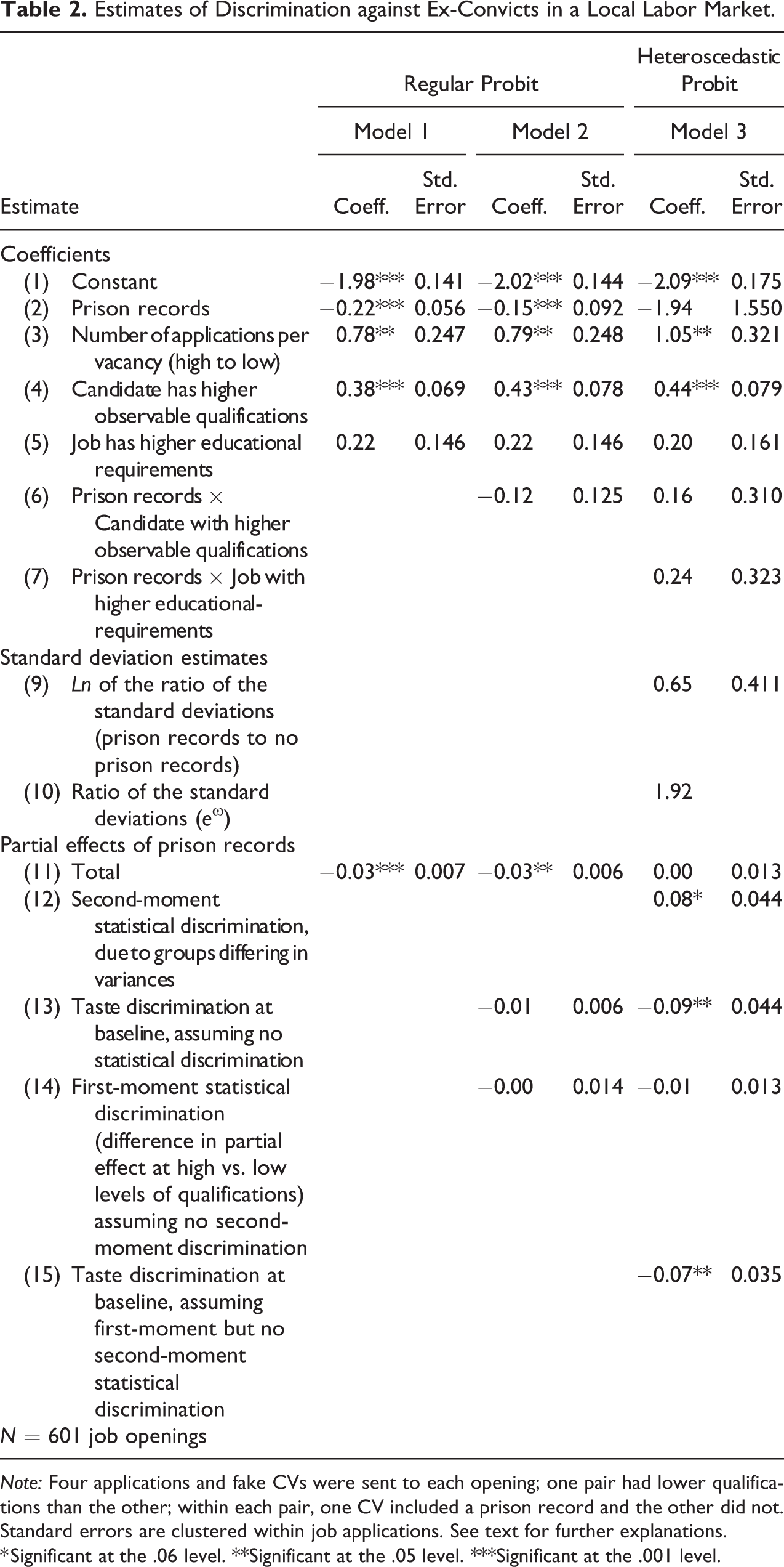
Table 2 presents the study’s main results. We focus on their methodological implications rather than their substantive interpretation. Standard errors for all models are clustered within jobs.

Table 2.

Estimates of Discrimination against Ex-Convicts in a Local Labor Market.

Estimate		Regular Probit				Heteroscedastic Probit
		Model 1		Model 2		Model 3
		Coeff.	Std. Error	Coeff.	Std. Error	Coeff.	Std. Error
Coefficients
(1)	Constant	−1.98***	0.141	−2.02***	0.144	−2.09***	0.175
(2)	Prison records	−0.22***	0.056	−0.15***	0.092	−1.94	1.550
(3)	Number of applications per vacancy (high to low)	0.78**	0.247	0.79**	0.248	1.05**	0.321
(4)	Candidate has higher observable qualifications	0.38***	0.069	0.43***	0.078	0.44***	0.079
(5)	Job has higher educational requirements	0.22	0.146	0.22	0.146	0.20	0.161
(6)	Prison records × Candidate with higher observable qualifications			−0.12	0.125	0.16	0.310
(7)	Prison records × Job with higher educational-requirements					0.24	0.323
Standard deviation estimates
(9)	Ln of the ratio of the standard deviations (prison records to no prison records)					0.65	0.411
(10)	Ratio of the standard deviations (e ^ω)					1.92
Partial effects of prison records
(11)	Total	−0.03***	0.007	−0.03**	0.006	0.00	0.013
(12)	Second-moment statistical discrimination, due to groups differing in variances					0.08*	0.044
(13)	Taste discrimination at baseline, assuming no statistical discrimination			−0.01	0.006	−0.09**	0.044
(14)	First-moment statistical discrimination (difference in partial effect at high vs. low levels of qualifications) assuming no second-moment discrimination			−0.00	0.014	−0.01	0.013
(15)	Taste discrimination at baseline, assuming first-moment but no second-moment statistical discrimination					−0.07**	0.035
N = 601 job openings

Note: Four applications and fake CVs were sent to each opening; one pair had lower qualifications than the other; within each pair, one CV included a prison record and the other did not. Standard errors are clustered within job applications. See text for further explanations.

* Significant at the .06 level. **Significant at the .05 level. ***Significant at the .001 level.

Model 1 shows the effect of having a prison record on the underlying variable $Y^{*}$ regulating callback probabilities, as estimated in a regular probit that has prison records as the main independent variable and applicant’s level of observables, job’s demand, and job’s required level of education as controls. The coefficient for prison records is significant and negative, like the corresponding partial or marginal effect of prison records on the probability of being selected (−.03). From these results, we conclude that there is discrimination against male ex-convicts. Their probability of being selected is three percentage points lower than for non-ex-convicts. Since the estimated probability of being selected is of only .06 overall, the difference translates into a substantial penalty for ex-convicts—they are one third less likely to be called back for further screening. The difficulty lies in isolating the mechanism driving such discrimination, which we do in models 2 and 3.

Model 2 aims at separating first-moment statistical discrimination from taste discrimination, without considering that there may also be second-moment statistical discrimination. We do it by adding to the previous regular probit an interaction effect between criminal records and applicant’s level of observables. We expect this interaction to provide a measure of how much employers rely on stereotypes about ex-convicts’ productivities linked to unobservables to select them. The interaction is negative, pointing toward an intensification of discrimination at higher levels of observables, but small and nonsignificant, also when expressed as a change in probability.

Model 3 is a heteroscedastic probit that allows callback variances to differ by group. This helps estimate second-moment statistical discrimination and identify the other two forms of discrimination without bias. We add two interaction effects between criminal records, on the one hand, and candidates’ observables and job educational requirements, on the other, to ensure that the estimate of the ratio of the variances is unaffected by employers’ beliefs that deficits in unobservables can be offset or exacerbated with higher observables.

Since employers apply different selection ratios in different jobs and select different proportions of applicants in each (see Table 1), the group with higher dispersion has a relative advantage in jobs with higher selection ratios that give more opportunities to unusual applicants. Model 3 (like models 1 and 2 before) shows that this group is made of ex-convicts, who have the highest relative variance (see row 10 in Table 2). Ex-convicts’ variance is almost twice as large as the other applicants’. The estimate is only significant when expressed as a marginal change in probability (row 12 in Table 2). We conclude that there is second-moment statistical discrimination and that ex-convicts benefit from it. The higher uncertainties that employers have about ex-convicts’ unobservables play to the latter’s advantage in jobs in which employers value more the unobserved qualifications of a candidate and increase their selection ratios to raise their chance to meet candidates with such unobservables. The effect is important. It increases ex-convicts callback probability by 9 percentage points (3 times their marginal probability).

Since there is heteroscedasticity, all estimates in models 1 and 2 were biased. The decomposition of taste and first-order statistical discrimination carried out in model 2 was also biased, if only slightly, as the interaction effect between criminal records and candidates’ levels of observables, and the corresponding group differences in the partial effects of observables, remain nonsignificant in model 3.

The most marked change is in the estimate of taste discrimination at baseline. We provide two such estimates—one discarding (row 13), and one considering (row 15), the nonsignificant difference in the partial effect of criminal records at the two levels of observables. In both cases, the marginal effect is significant and negative. Ex-convicts experience taste discrimination. Its impact on their probability of being selected is important, as the penalty is more than three times the marginal penalty estimated for ex-convicts in model 1, which included all forms of (positive and negative) discrimination.

The results indicate that in the local market that we studied, employers discriminate against ex-convicts on moral grounds. Were it not because employers think that an average ex-convict is as productive as another based on their unobservables (although they can predict such productivity less accurately for ex-convicts), and were it not because in this market they give higher weight to unobservables, widening the range of candidates considered for an interview, the discrimination of ex-convicts on the grounds of their moral wrongdoings would be revealed in its true magnitude.

Table 3 shows the results of sensitivity analyses aimed at assessing the robustness of the findings and the plausibility of the assumptions on which they lie. In model 4, we show the results of using a proxy for the number of applications per vacancy instead of the actual number to estimate the selection cutoff and the ratio of the variances of the two groups. As noted, many search engines omit this number in the job offer. However, they often publish reports on the number of applications processed in a term (typically a year) broken by sector. Our proxy assigns to each job the sum of the mean number of applications received by jobs in the same sector and year (in z scores times −1)¹⁷ and of the proportion of callbacks received among the pool of applications sent to each job (also in z scores). The latter—we argued above—should increase as applications decrease. Row 12 of Table 3 reports the results of a Wald test comparing the fit of model 3 in Table 1, which uses the actual number of applications per vacancy, with that of model 4 in Table 3, which uses the proxy just described. The differences are not significant. We conclude that our method is robust to using aggregate information on the number of applications per sector.

Table 3.

Sensitivity Analyses.

Estimates and Tests		Heteroscedastic Probit		Heteroscedastic Ordered Probit		Regular Probits
		Model 4		Model 5		Model 6		Model 7		Model 8
		Coeff.	Std. Error	Coeff.	Std. Error	Coeff.	Std. Error	Coeff.	Std. Error	Coeff.	Std. Error
Coefficients
(1)	Constant	−3.37***	0.516	0^a		−2.09***	0.175	−2.06***	0.151	−2.15*	1.245
(2)	Prison records	−0.77	0.491	−1.01	1.550	0.01	0.183	−0.08	0.200	0.98	1.361
(3)	Less demanded job (fewer applications per vacancy)			0.95**	0.325	1.06**	0.321	1.05***	1.053	2.51	2.716
(4)	Candidate has higher observable qualifications	1.67***	0.402	0.43***	0.080	0.44***	0.079	0.38***	0.088	−0.12	0.313
(5)	Job has higher educational requirements	−0.62**	0.212	0.21	0.158	0.2	0.161	0.20	0.134	−0.31	0.466
(6)	Prison records × Candidates with higher qualifications	−0.63	0.496	0.02	0.233	−0.13	0.124
(7)	Prison records × Job with higher educational requirements	−0.2	0.458	0.12	0.219	0.03	0.143	0.03	0.203	0.41	0.751
(8)	Proxy for less demanded job^b	1.22**	0.316
(9)	Prison records × Proxy for less demanded job					−0.51*	0.302	0.50	0.311	−2.86	2.782
Standard deviation estimates
(10)	Ln of the ratio of the standard deviations (CR to NCR)	0.48**	0.152	0.36	0.337
(11)	Ratio of the standard deviations (e ^ω)	1.61		1.44
Tests										Wald/t test	Prob.
The models estimated with the actual and the approximated number of applications per vacancy are equivalent
(12)	H₀: Fit of model 4 in Table 3 = Fit of model 3 in Table 2									0.43	0.513
Neumark’s homogeneity test: the ratio of the effect of the control variable in each group equals the ratio of the effect of # of applicants in each group
(13)	H₀: (3)/[(3)+(9)] in Model 6 = (5)/[(5)+(7)] in model 6									1.06	0.302
Threshold selection model test: Candidates’ higher qualifications affect if they are selected but not the order in which they are selected
(14)	H₀: (4) in model 8 ≤ (4) in model 7									1.81	0.035^c

^a Parameters estimate for higher cutoffs are available upon request.

^b Index created by adding the standardized scores of “mean # of yearly applications in jobs within the same sector” to the “# of callbacks in each job applied for” times −1.

^c Probability for a directional z test.

* Significant at the .10 level. **Significant at the .05 level. ***Significant at the .001 level.

In model 5, we reestimate model 3 of Table 1 using another type of heterogeneous choice models—a heteroscedastic ordered probit (Williams 2009)—which corrects for the impact that omitting relevant independent variables has on the scaling of the variance at baseline in probit models (Mood 2010). It does so by reestimating coefficients net of the value of the constant (Williams 2009, 2010). Because we sent four CVs to each job and recorded the date and time when each applicant received a callback (if he did), we could generate a new dependent variable measuring the call order—from 0 (never called) to 4 (called in first place). Because there were very few cases in which all four fake applicants were selected, we recoded the variable into three values (1 = never called, 2 = called in fourth or third place, and 3 = called in second or first place). As shown in model 5, while there are some changes in the estimates of the independent variables, they are minor, confirming that the results are robust.

In row 13 of Table 3, we report results from a homogeneity tests evaluating the assumption that the interaction effect between the number of applicants per opening and group membership is driving the ratio of the group variances calculated in model 3 of Table 2. If it did, as noted by Neumark (2012) and discussed before, the ratio of the effect of the number of applicants per opening among non-ex-convicts and ex-convicts should approximate the ratio of the effect of job’s educational requirements in each group in the full two-way interaction probit model 6 of Table 3 (this is just a reparametrization of the heteroscedastic model run in model 3 of Table 2). Test results are reassuring since the differences are insignificant.

Finally, in row 14 of Table 3, we report the results of testing the validity of the threshold model of selection, one where candidates’ merits are relevant for predicting their being selected but not the order in which they are selected. The results of the test are significant and in the expected direction, giving more credence to the interpretation that group differences in the effect of candidates’ qualifications on their appeal to employers indicate the presence of first-order statistical discrimination.

Summary and Discussion

In this article, we discussed some important interpretative problems associated with correspondence studies aimed at measuring labor market discrimination and proposed a comprehensive method to solve them. We reviewed and reformalized the two problems that make it difficult to interpret minorities’ typically lower selection rates as indicating that employers distaste them and apply a higher selection cutoff to them. First, lower rates may indicate that employers perceive minorities to have lower average productivities linked to unobservables, leading to first-moment statistical discrimination. Second, employers might perceive minorities to be more or less similar to each other in unobservables than nonminorities. Depending on which group is perceived as having higher variance and on how high do employers set the selection cutoff, higher or lower callback rates may ensue—a case of second-moment statistical discrimination.

Neumark (2012) proposed a solution to separate second-moment statistical discrimination from the other two by introducing variation in applicants’ levels of observables. This variation, he argued, allows estimating the relative ratio of groups’ variances in a heteroscedastic probit model. If employers selected larger proportions of applicants with higher observables, any relative differences across groups in how much or less candidates with different observables are likely to be selected should provide an estimate of the ratio of groups’ variances and of second-moment statistical discrimination.

We questioned Neumark’s reliance on variations in the intensity of discrimination at different levels of observables to estimate second-moment statistical discrimination, since these variations could also reflect employers’ perceptions of groups’ different average productivities linked to unobservables. Instead, we proposed to rely on variations in the intensity of discrimination across jobs differing in the number of applicants. This number has been shown to alter employers’ selection ratios and the weight given to unobservables in their hiring strategies—higher when selecting more candidates for screening. Variations in the level of discrimination across jobs with different selection ratios help identify the group with the largest variance—the one benefitting the most from higher selection ratios—and estimate second-moment statistical discrimination. The plausibility of alternative explanations can be tested using Neumark homogeneity test (2012).

In contrast, we relied on variations in the level of discrimination at different levels of observables to identify first-moment statistical discrimination. Such an interaction effect should be expected if employers selected for further screening all (or the first n) applicants that pass a minimum qualification threshold, rather than in order of qualifications, and if they thought that groups differ in productivities, as measured in some composite index where deficits in unobservables can be (partly) compensated with surpluses in observables. We proposed to test the plausibility of the threshold model of selection by observing if among the selected candidates those with higher qualifications are called first. If they did not, this would give more credence to the claim that differences in the level of discrimination across candidates with different observables capture first-moment statistical discrimination.

Our main contribution has been to integrate both procedures into a unified heteroscedastic probit model that makes the variance a function of group membership. In this model, taste discrimination is estimated residually, as discrimination that cannot be accounted for by stereotypes about the distribution of unobservables across groups. We showed how to estimate it depending on the direction and intensity of the two forms of statistical discrimination.

Applying this method, we uncovered a credible story about the sources of discrimination against ex-convicts in a local market. We showed that this discrimination was based on aversion (distaste) toward ex-convicts due to their past wrongdoings, not on higher uncertainties about their unobserved qualifications, which instead played to their advantage, and not on stereotypes about their average productivities, which were perceived to be similar to non-ex-convicts’. This has policy implications. Tackling distaste toward ex-convicts may be difficult and affect ex-convicts’ chances of regaining a decent life and avoid reoffending. More research is necessary to ascertain if channeling ex-convicts toward jobs in which certified qualifications are less important, and where they have higher chances of being hired, could help overcome their stigma.

Our method to separate the three forms of discrimination can be improved by minimizing measurement and specification errors, especially since heteroscedastic models are notorious for magnifying them (Keele and Park 2006). First, the variables in the model could be better measured. The dependent variable could be measured ordinally, by reporting the callback order of the candidates in designs that send more than two applications to each job, as we did in the sensitivity analyses. Applicants’ observables could be measured on an interval scale, rather than as a dichotomy, making the test of the interaction effect between group membership and the level of observables less dependent on tester’s choices.

Second, more variables could be added to better measure each form of discrimination. For example, in well budgeted studies, it might be possible to alternate different qualification across candidates applying to similar jobs and test their contribution to explaining first-moment statistical discrimination. Other job characteristics could be used to construct proxies of jobs’ selection ratios when the number of applicants in each is unavailable. We provided an example in the sensitivity analyses by using a proxy that combined the rate of callbacks obtained in each job with the average number of candidates applying for jobs in the same sector.

Third, miss-specification tests could also be refined. Neumark’s (2012) homogeneity tests, as he himself proposed, could be applied to subsets of controls which effects are unlikely to change across groups for reasons different to their variance, like some random variables used in the study (application order, pictures assigned to applicants, etc.). The test of the threshold model of selection could be complemented with another directly testing for the exchangeability of unobservables and observables. For example, the tester could add some unobservables to some candidates CV’s and observe how their impact on selection probabilities changes as candidates’ observables are experimentally modified.

While there is room for improvement, we hope to have contributed to strengthening the methodological foundations of correspondence studies and discrimination research.

Footnotes

Declaration of Conflicting Interests

The author(s) declared no potential conflicts of interest with respect to the research, authorship, and/or publication of this article.

Funding

The author(s) disclosed receipt of the following financial support for the research, authorship, and/or publication of this article: Grant RecerCaixa 2013. “La regulación de los antecedentes penales”. Funded by La Caixa and ACUP.” Grant DER2015-64403-P. “Enforcement and supervision of sentences”. Funded by the Spanish Ministry of Economy & Competitiveness and FEDER (EU).

ORCID iD

Jorge Rodríguez Menés

Notes

References

Ahmed

Ali M.

Andersson

Lina

Hammarstedt

Mats

. 2010. “Can Discrimination in the Housing Market Be Reduced by Increasing the Information about the Applicants?” Land Economics 86:79–90.

Alós-Moner

Ramón

Esteban

Fernando

Jodar

Pere

Miguélez

Fausto

Alcaide

Vanessa

López-Roldan

y Pedro

. 2011. “La inserció laboral dels exinterns dels centres penitenciaris de Catalunya.” Documents de treball del Centre d’Estudis Jurídics i Formació Especialitzada (CEJFE). Barcelona: Centre d’Estudis d’Opinió i Formació Especialitzada (CEJFE).

Altonji

Jospeph G.

Pierret

Charles R.

. 2001. “Employer Learning and Statistical Discrimination.” The Quarterly Journal of Economics 116:313–50.

Anderson

Donna M.

Haupert

Michael J.

. 1999. “Employment and Statistical Discrimination: A Hands-on Experiment.” The Journal of Economics 25:85–103.

Becker

Gary S.

1971. The Economics of Discrimination. 2nd Ed. Chicago, IL: University of Chicago Press.

Bertrand

Marianne

Mullainathan

Sendhil

. 2004. “Are Emily and Greg More Employable than Lakisha and Jamal? A Field Experiment on Labor Market Discrimination.” The American Economic Review 94:991–1013.

Booth

Alison L.

Leigh

Andrew

Varganova

Elena

. 2012. “Does Ethnic Discrimination Vary across Minority Groups? Evidence from a Field Experiment.” Oxford Bulletin of Economics and Statistics 74:547–73.

Bosch

Mariano

Angeles Carnero

Farre

Lidia

. 2010. “Information and Discrimination in the Rental Housing Market: Evidence from a Field Experiment.” Regional Science and Urban Economics 40:11–19.

Carlsson

Eriksson

. 2017. “The Effect of Age and Gender on Labor Demand. Evidence from a Field Experiment.” Working paper series: Linnaeus University Centre for Discrimination and Integration Studies 2017: 4.

10.

Castillo

Marco

Petrie

Ragan

. 2010. “Discrimination in the Lab: Does Information Trump Appearance?” Games and Economic Behavior 68:50–59.

11.

Connerley

Mary L.

2013. “Recruiter Effects and Recruitment Outcomes.” Pp. 21–34 in The Oxford Handbook of Recruitment, edited by Yu

K. Y. T.

Cable

D. M.

. Oxford, UK: Oxford University Press.

12.

Cornelißen

Thomas

. 2005. “Standard Errors of Marginal Effects in the Heteroskedastic Probit Model.” Diskussionspapiere des Fachbereichs Wirtschaftswissenschafte nº 320. Hannover, Germany: Universität Hannover.

13.

Correll

Shelley J.

Benard

Stephen

Paik

. 2007. “Getting a Job: Is There a Motherhood Penalty?” American Journal of Sociology 112:1297–339.

14.

De Corte

Wifried

Lievens

Filip

Sackett

Paul R.

. 2007. “Combining Predictors to Achieve Optimal Trade-offs between Selection Quality and Adverse Impact.” Journal of Applied Psychology 92:1380–93.

15.

DeLiema

Marguerite

Yon

Yongjie

Wilber

Kathleen H.

. 2016. “Tricks of the Trade: Motivating Sales Agents to Con Older Adults.” The Gerontologist 56:335–44.

16.

Drydakis

Nick

. 2014. “Sexual Orientation Discrimination in the Cypriot Labour Market. Distastes or Uncertainty?.” International Journal of Manpower 35: 720–44.

17.

Dymski

Gary A.

2006. “Discrimination in the Credit and Housing Markets: Findings and Challenges.” Pp. 215–59 in Handbook on the Economics of Discrimination, edited by Rodgers

W. M.

. Northampton, MA: Edward Elgar.

18.

Ewens

Michael

Tomlin

Bryan

Wang

Liang Choon

. 2014. “Statistical Discrimination or Prejudice? A Large Sample Field Experiment.” Review of Economics and Statistics 96:119–34.

19.

Fershtman

Chaim

Gneezy

Uri

. 2001. “Discrimination in a Segmented Society: An Experimental Approach.” The Quarterly Journal of Economics 116:351–77.

20.

Finch

David M.

Edwards

Bryan D.

Craig Wallace

. 2009. “Multistage Selection Strategies: Simulating the Effects on Adverse Impact and Expected Performance for Various Predictor Combinations.” Journal of Applied Psychology 94:318–40.

21.

Greene

William H

. 2010. “Testing Hypotheses about Interaction Terms in Nonlinear Models.” Economics Letters 107:291–96.

22.

Greene

William H.

Hensher

David A.

. 2010. Modeling Ordered Choices: A Primer and Recent Developments. Cambridge, UK: Cambridge University Press.

23.

Guryan

Jonathan

Charles

Kerwin K.

. 2013. “Taste-based or Statistical Discrimination: The Economics of Discrimination Returns to Its Roots.” The Economic Journal 123:F417–43.

24.

Heckman

James J.

1998. “Detecting Discrimination.” Journal of Economic Perspectives 12:101–16.

25.

Heckman

James J.

Siegelman

Peter

. 1993. “The Urban Institute Audit Studies: Their Methods and Findings”, in Clear and Convincing Evidence: Measurement of Discrimination in America, edited by Michael

Fix

Struyk

Raymond J.

. Washington, DC: The Urban Institute Press.

26.

InfoJobs and ESADE. 2013. “Informe InfoJobs ESADE. Estado del mercado laboral en España.” Retrieved November 8, 2017 (https://nosotros.infojobs.net/wp-content/uploads/informe-infojobs-esade-2012-1.pdf).

27.

Kaas

Leo

Manger

Christian

. 2012. “Ethnic Discrimination in Germany’s Labour Market: A Field Experiment.” German Economic Review 13:1–20.

28.

Keele

Luke

Park

David K.

. 2006. “Difficult Choices: An Evaluation of Heterogeneous Choice Models.” Working Paper prepared for the 2004 Meeting of the American Political Science Association. 2nd version. Retrieved April 21, 2017 (http://www.nd.edu/∼rwilliam/oglm/ljk-021706.pdf).

29.

Keinert-Kisin

Christina

Hatzinger

Reinhold

Köszegi

Sabine T.

. 2012. “What’s in a Name? A Personnel Selection Experiment on Gender Bias in Applicant Assessment.” Paper presented at the EGOS (European Group of Organization Studies) Colloquium 2012, July 5, Helsinki, Sweden. Retrieved October 6, 2017 (https://www.semanticscholar.org/paper/What-s-in-a-Name-a-Personnel-Selection-Experiment-Keinert-Kisin-Hatzinger/650e60d93323d8644390ce621c8d8ccac3ab9a28).

30.

Lahey

Joanna N.

2008. “Age, Women, and Hiring an Experimental Study.” Journal of Human Resources 43:30–56.

31.

Lahey

Joanna N.

Oxley

Douglas

. 2016. “Discrimination at the Intersection of Age, Race, and Gender: Evidence from a Lab-in-the-field Experiment.” National Bureau of Economic Research Working Paper Series, No. 25357.

32.

Lang

Kevin

Lehmann

Jee-Yeon K

. 2012. “Racial Discrimination in the Labor Market: Theory and Empirics.” Journal of Economic Literature 50:959–1006.

33.

Huy

In-Sue

Shaffer

Jonathan

Schmidt

Frank

. 2007. “Implications of Methodological Advances for the Practice of Personnel Selection: How Practitioners Benefit from Meta-analysis.” The Academy of Management Perspectives 21:6–15.

34.

Levitt

Stephen D.

2004. “Testing Theories of Discrimination: Evidence from Weakest Link.” Journal of Law and Economics 47:431–52.

35.

List

John A.

2004. “The Nature and Extent of Discrimination in the Marketplace: Evidence from the Field.” The Quarterly Journal of Economics 119:49–89.

36.

Masclet

David

Pererle

Emmanuel

Larribeau

Sophie

. 2012. “The Role of Information in Deterring Discrimination: A New Experimental Evidence of Statistical Discrimination.” Working Paper No. 201238. Rennes: Center for Research in Economics and Management (CREM), University of Rennes 1, University of Caen and CNRS. Retrieved October 6, 2017 (https://crem-doc.univ-rennes1.fr/wp/2012/201238.pdf).

37.

Mood

Carina

. 2010. “Logistic Regression: Why We Cannot Do What We Think We Can Do, and What We Can Do About It.” European Sociological Review 26:67–82.

38.

Neumark

David

. 2012. “Detecting Discrimination in Audit and Correspondence Studies.” Journal of Human Resources 47:1128–57.

39.

Neumark

David

. 2016. “Experimental Research on Labor Market Discrimination.” National Bureau of Economic Research Working Papers Series, No. 22022.

40.

Norton

Edward C.

Wang

Hua

Chunrong

. 2004. “Computing Interaction Effects and Standard Errors in Logit and Probit Models.” Stata Journal 4:154–67.

41.

Pager

Devah

. 2003. “The Mark of a Criminal Record.” American Journal of Sociology 108:937–75.

42.

Pager

Devah

Quillian

Lincoln

. 2005. “Walking the Talk? What Employers Say versus What They Do.” American Sociological Review 70:355–80.

43.

Phillips

Katherine W.

Rothbard

Nancy P.

Dumas

Tracy L

. 2009. “To Disclose or Not to Disclose? Status Distance and Self-disclosure in Diverse Environments.” Academy of Management Review 34:710–32.

44.

Rich

Judith

. 2014. “What Do Field Experiments of Discrimination in Markets Tell Us? A Meta Analysis of Studies Conducted Since 2000.” IZA Discussion Paper Nº 8584. Retrieved November 7, 2017 (https://ideas.repec.org/p/iza/izadps/dp8584.html).

45.

Rohwer

Goetz

. 2015. “A Note on the Heterogeneous Choice Model.” Sociological Methods & Research 44:145–48.

46.

Rudman

Laura A.

Moss-Racusin

Corinne A.

Phelan

Julie E.

Julie

Nauts

Sanne

. 2012. “Status Incongruity and Backlash Effects: Defending the Gender Hierarchy Motivates Prejudice against Female Leaders.” Journal of Experimental Social Psychology 48:165–79.

47.

Sackett

Paul R.

Schmitt

Neal

Ellingson

Jill

Kabin

Melissa B.

. 2001. “High-stakes Testing in Employment, Credentialing, and Higher Education: Prospects in a Post-affirmative-action World.” American Psychologist 56:302–18.

48.

Schmidt

Frank L.

Hunter

John E.

. 1998. “The Validity and Utility of Selection Methods in Personnel Psychology: Practical and Theoretical Implications of 85 Years of Research Findings.” Psychological Bulletin 124:262–72.

49.

Uggen

Chris

Vuolo

Mike

Lageson

Sarah

Ruhland

Ebony

Whitham

Hilary K.

. 2014. “The Edge of Stigma: An Experimental Audit of the Effects of Low-level Criminal Records on Employment.” Criminology 52:627–54.

50.

Weichselbaumer

Doris

. 2004. “Is It Sex or Personality? The Impact of Sex Stereotypes on Discrimination in Applicant Selection.” Eastern Economic Journal 30:159–86.

51.

Williams

Richard

. 2009. “Using Heterogeneous Choice Models to Compare Logit and Probit Coefficients across Groups.” Sociological Methods & Research 37:531–59.

52.

Williams

Richard

. 2010. “Fitting Heterogeneous Choice Models with Oglm.” Stata Journal 10:540–67.

53.

Yinger

John

. 1998. “Evidence on Discrimination in Consumer Markets.” Journal of Economic Perspectives 12:23–40.

54.

Zschirnt

Eva

Ruedin

Didier

. 2016. “Ethnic Discrimination in Hiring Decisions: A Meta-analysis of Correspondence Tests 1990–2015.” Journal of Ethnic and Migration Studies 42:1115–34.

55.

Zussman

Asaf

. 2013. “Ethnic Discrimination: Lessons from the Israeli Online Market for Used Cars.” The Economic Journal 123:F433–68.