
Abstract
Often in sociology, researchers are confronted with nonnormal variables whose joint distribution they wish to explore. Yet, assumptions of common measures of dependence can fail or estimating such dependence is computationally intensive. This article presents the copula method for modeling the joint distribution of two random variables, including descriptions of the method, the most common copula distributions, and the nonparametric measures of association derived from the models. Copula models, which are estimated by standard maximum likelihood techniques, make no assumption about the form of the marginal distributions, allowing consideration of a variety of models and distributions in the margins and various shapes for the joint distribution. The modeling procedure is demonstrated via a simulated example of spousal mortality and empirical examples of (1) the association between unemployment and suicide rates with time series models and (2) the dependence between a count variable (days drinking alcohol) and a skewed, continuous variable (grade point average) while controlling for predictors of each using the National Longitudinal Survey of Youth 1997. Other uses for copulas in sociology are also described.
Keywords
Introduction
Often in sociology, researchers are confronted with nonnormal variables whose joint distribution they wish to explore. Yet, assumptions of common measures of dependence can fail or estimating such dependence is computationally intensive. For these reasons, joint distributions, which define the probability of events in terms of two or more variables (i.e., the probability of two variables simultaneously having particular values), receive little attention in sociology. Rather, sociologists tend to focus on conditional distributions as given through methods based upon generalized linear models, which describe the probability across a univariate distribution when the value of another variable is known (i.e., the probability of a dependent variable given that an independent variable(s) has a certain value). This article presents the copula method for modeling the joint distribution of two random variables. Put most simply, copulas are joint distribution functions that “couple” one-dimensional marginal distribution functions together, defining the probability space across the values of both marginals (Nelsen [1998] 2006:1). Copulas accomplish the modeling of joint distributions by making the cumulative distribution functions (CDFs) of each marginal the object of analysis.
While techniques for joint multivariate normal distributions are well developed, copula models provide a technique for analyzing joint nonlinear distributions of nonnormal data, which arises frequently in sociology. This is advantageous for several reasons (Joe 1997; Frees and Valdez 1998; Nelsen 2006; Trivedi and Zimmer 2007). Sociologists have techniques for modeling nonlinear marginal distributions (e.g., via various generalized linear models), but lack straightforward methods for deriving joint distributions of those marginal distributions, which copulas provide. Copula modeling affords the researcher the ability to model each marginal differently, providing much flexibility in model specification and a valuable feature given the variety of empirical distributions encountered in sociological data. Estimating the joint distributions of nonlinear outcomes is often computationally demanding and requires the use of simulation, whereas copula models are fit via standard maximum likelihood procedures. Following this modeling, copulas provide a unit-free, nonparametric measure of dependence (alternatively called association or mixture) that is general and free from influence of the specific marginal distributions, going beyond correlation or linear association. The dependence parameter, along with the parameters of the marginal distributions, are then used to provide an estimate of the joint probability, which can exhibit different strengths across the joint distribution.
This technique has demonstrated utility in fields such as actuarial science (e.g., Frees and Valdez 1998, 2008; Frees and Wang 2005; Frees, Carriere, and Valdez 1996), finance (e.g., Cherubini, Luciano, and Vecchiato 2004; McNeil, Frey, and Embrechts 2005), economics (e.g., Cameron et al. 2004; Smith 2005; Trivedi and Zimmer 2007), marketing (e.g., Danaher and Smith 2011), medicine (e.g., Escarela and Carriere 2003; Wang and Wells 2000), and engineering (e.g., Genest and Favre 2006; Salvadori et al. 2007).
Copulas are particularly useful for sociologists in several situations. First, much data in sociology is nonnormal and often highly skewed. After finding the appropriate distributions for the two outcomes of interest, one can use a copula to understand the association between these two variables. A simulated example examining the dependent mortality of husbands and wives is used subsequently to illustrate this point. Given the skewness of these variables, copulas are particularly useful in examining behavior of heavy-tailed data. As such, sociologists could use these methods for the joint probability of events that may be rare in occurrence. The copula model, however, is much more general. In sociology, we often do not know the causal order of outcomes, including among complex time series data, yet still wish to accurately model a multivariate relationship while controlling for predictors of interest for each outcome. In modeling each marginal separately and applying a copula to understand the multivariate distribution, this becomes a possibility. An example of time series marginals for unemployment and suicide rates follows subsequently. Researchers can also construct separate marginal distributions based upon generalized regression models and examine the relationship between various phenomena using a copula. In an example using National Longitudinal Survey of Youth 1997 (NLSY97) data, the relationship between a skewed continuous measure and count data with covariates in the margins is shown in order to attest to the generality of the method. Additional potential uses for copulas within sociology are also described.
In what follows, I first describe the copula methodology, providing the definition of a copula and examples of several types of copula distributions. Then, as mentioned earlier, I show examples of the modeling procedure. First, I generate simulated data as a simple example of model fitting, model selection, association, and joint probabilities. Second, I present an empirical example with time series in the margins. Third, I show an example with generalized linear models in the margins. Then, I outline additional possible uses for sociologists. Finally, I revisit the usefulness of copulas, while also pointing to some of the limitations.
Introduction to Copula Models
Definition
The mathematics for copulas is presented elsewhere, but the main concepts are summarized here. For simplicity, only the bivariate case is discussed (for a complete treatment of the mathematics, see Joe 1997 and Nelsen 2006; for other discipline-specific introductions, see Frees and Valdez 1998; Genest and Favre 2006; Trivedi and Zimmer 2007). In the bivariate case, suppose we have two variables of interest y 1 and y 2. Their CDFs are then denoted as F1(y1) and F2(y2), and their joint CDF is denoted as F(y1,y2). A copula function uses the CDFs as the object of analysis or the inputs. The definition of the copula is derived from the work of Sklar (1959; see also Schweizer and Sklar 1974). According to Sklar’s (1959) Theorem, for any joint distribution F(y1,y2) with marginal cumulative distributions F1(y1) and F2(y2), there exists a copula function

In other words, the joint distribution of any two outcomes y 1 and y 2 can be expressed as a copula function that is determined only by the individual marginal CDFs F1(y1) and F2(y2) and an association parameter θ that binds them together. Given that CDFs are bound between 0 and 1 by definition, the function takes a value on the unit square and produces a value on the unit interval. 1 To summarize, we input the values for each of the marginals (y 1 and y 2) into its respective CDF (F 1 and F 2) to produce a value on the unit line (denoted u and v, respectively), which inputted into a copula function provides their joint distribution.
For any two continuous marginals, the CDF is uniform from 0 to 1, or
Schweizer and Wolff (1981) showed that the copula captures all of the dependence between two random variables via two standard nonparametric measures of association, namely Spearman’s ρ and Kendall’s τ. This surprising conclusion results from the fact that (1) the joint distribution can be decomposed into the marginal distributions and the copula, and (2) each of these measures of association can be expressed solely in terms of the copula function. They further show that Pearson’s correlation coefficient does not satisfy the latter, such that it does not provide an accurate measure of dependence only, due to also containing information from each of the marginals. Thus, Spearman’s ρ and Kendall’s τ can be applied to the joint distribution regardless of the specific form of the marginal distributions and have been shown to take all values in the desired interval [−1,1], but both conditions are not always satisfied for Pearson’s correlation 2 (Embrechts, McNeil, and Straumann 2002). Among the most useful results, the copula allows the strength of the relationship of the two marginals to change across the joint distribution, as can be seen in the several examples of types of copulas. For the association parameters, the square of Spearman’s ρ can be interpreted similar to Pearson’s correlation as the percentage of shared or explained variance, while Kendall’s τ can be interpreted as the difference in the probability of the two variables being in the same order versus the probability of not being in the same order. For the case of two discrete marginal distributions, the occurrence of ties could decrease the attainable value of the measure of association (see Denuit and Lambert 2005; Trivedi and Zimmer 2007:24-25). Thus, it is crucial that the marginal distributions are first modeled accurately. With a better fit of the margins, one can model the dependence structure more precisely (Trivedi and Zimmer 2007:62). Luckily, this step is one with which sociologists are quite familiar, as it encompasses the modeling techniques that are standard to the discipline.
Copula modeling allows researchers to consider the marginal modeling and dependence modeling as separate but related issues through several straightforward steps. First, choose the appropriate marginal distributions, which need not be the same for each marginal distribution, and estimate the distributional parameters via maximum likelihood. Importantly, there is no restriction on the distribution of the margins. This step is akin to model selection for each marginal and can be a simple chosen distribution that appears to fit the data well or an actual generalized regression model.
Second, we need to transform the observed data to its CDF. This conversion is known as the probability integral transformation, though the procedure is more straightforward than the name suggests. 3 The transformation applies a given distribution to data in order to produce the probability of observing an equal or lower value. In essence then, this procedure is the same as finding a p value (technically 1 − p value, or the “complement” of the p value; that is, the probability up to that point, rather than beyond it). The uniform distribution of the CDFs on the unit line is only guaranteed if the marginal distribution is correct. In the case of empirical data, researchers must check this uniformity, which may not exist if the marginal distribution is incorrectly specified, attesting to the importance of fitting the margins correctly. The following example with grade point average (GPA) will demonstrate this importance.
Third, using the starting values from the estimation of the parameters of the margins once an appropriately fitting distribution is selected, estimate the copula model, including the association parameter and all the marginal parameters, by maximum likelihood. There are several types of copulas discussed subsequently and researchers should fit many using model selection techniques to choose the best fitting copula.
Finally, measures of dependence are computed from the best fitting copula model. We can then convert the dependence parameter into the well-known measures of association of Kendall’s τ and Spearman’s ρ, providing a measure of the strength of the joint relationship, which, together with the appropriate copula function, provide the joint distribution free of influence from the marginal distributional forms. Since the copula is a probability distribution, we can input the cumulative probabilities calculated from each marginal distribution into the best fitting copula model to produce joint probabilities.
Types of Copulas
Although the distributional forms of copulas may appear unfamiliar to sociologists, they are analogous to any other parametric joint distribution, but conforming to the above mentioned definition and properties. As with the distributions that are familiar, there are many distributions that satisfy those assumptions. In this section, I describe the most common copula distributions within three distributional families. Families share a common underlying formula, with differences dictated by a “generator” function which is plugged into that formula. For simplicity, the discussion is restricted to the bivariate case.
The first family is the elliptical family of copulas (see, e.g., Durante and Sempi 2010:14-15). The members of the elliptical family are derived from the density function of an elliptical distribution with mean zero and correlation matrix Σ which is given, for every
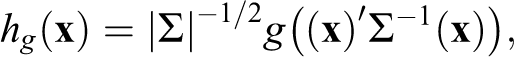
where g is a generator function. The two most common elliptical copulas are the Normal (or Gaussian) copula and the t-copula. Table 1 gives several examples of bivariate copulas. The third column of the table shows the generator function g(t). For example, the generator function for the bivariate Normal copula is
Select Common Bivariate Copulas (Nelsen 2006).
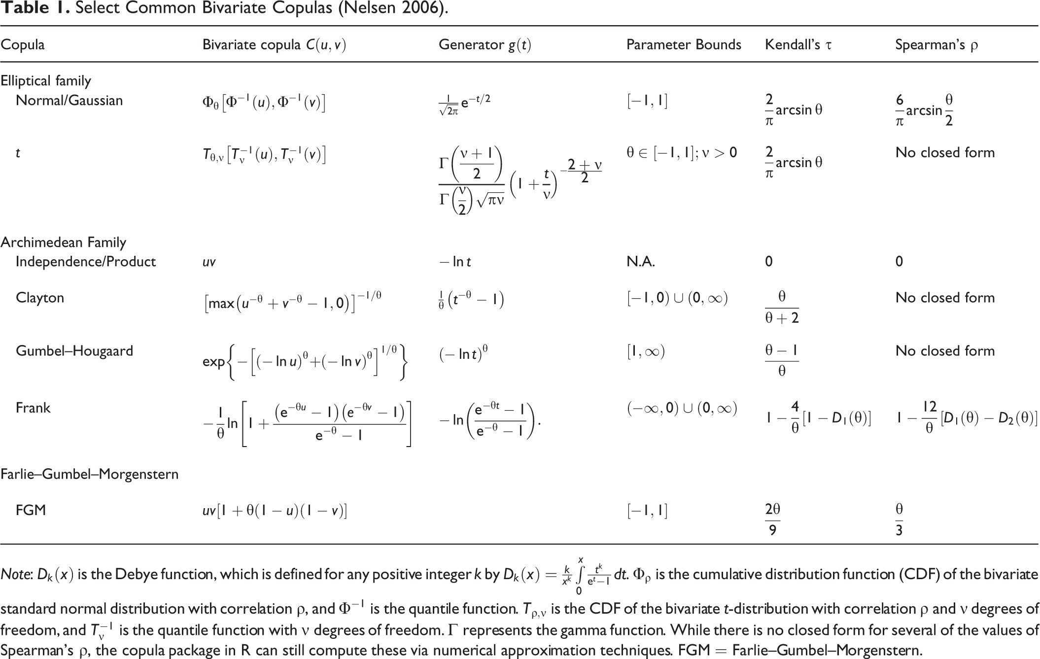
Note:
The Normal copula is an important starting point since normal marginal distributions result in the Normal copula reducing to the familiar multivariate normal distribution. In the case of elliptical marginal distributions (as would arise with normal margins), we can interpret the association parameter for elliptical copulas as the linear correlation. With more diverse margins of interest, there is a need for other measures of association because the correlation is not free of influence from the form of the marginal distributions. As described earlier, Kendall’s τ and Spearman’s ρ provide such measures and are given in Table 1. In the case of the Normal copula, Kendall’s τ provides a nonparametric robust and efficient estimator of association for both elliptical and non-elliptical margins (Embrechts, Lindskog, and McNeil 2003:357-60). Figure 1 depicts the CDF and probability distribution function (PDF) for the Normal copula with various association parameters. At the lower depicted relationship (τ = 0.16), the probability is more evenly distributed over all the values of both margins. While the relationship is strongest among the lowest and highest values of each marginal, there is room for considerable discordance. As the value of Kendall’s τ increases, the concordance increases, reserving the most probability along the main diagonal. A negative association would put the highest probabilities in the opposite corners (i.e., discordance).
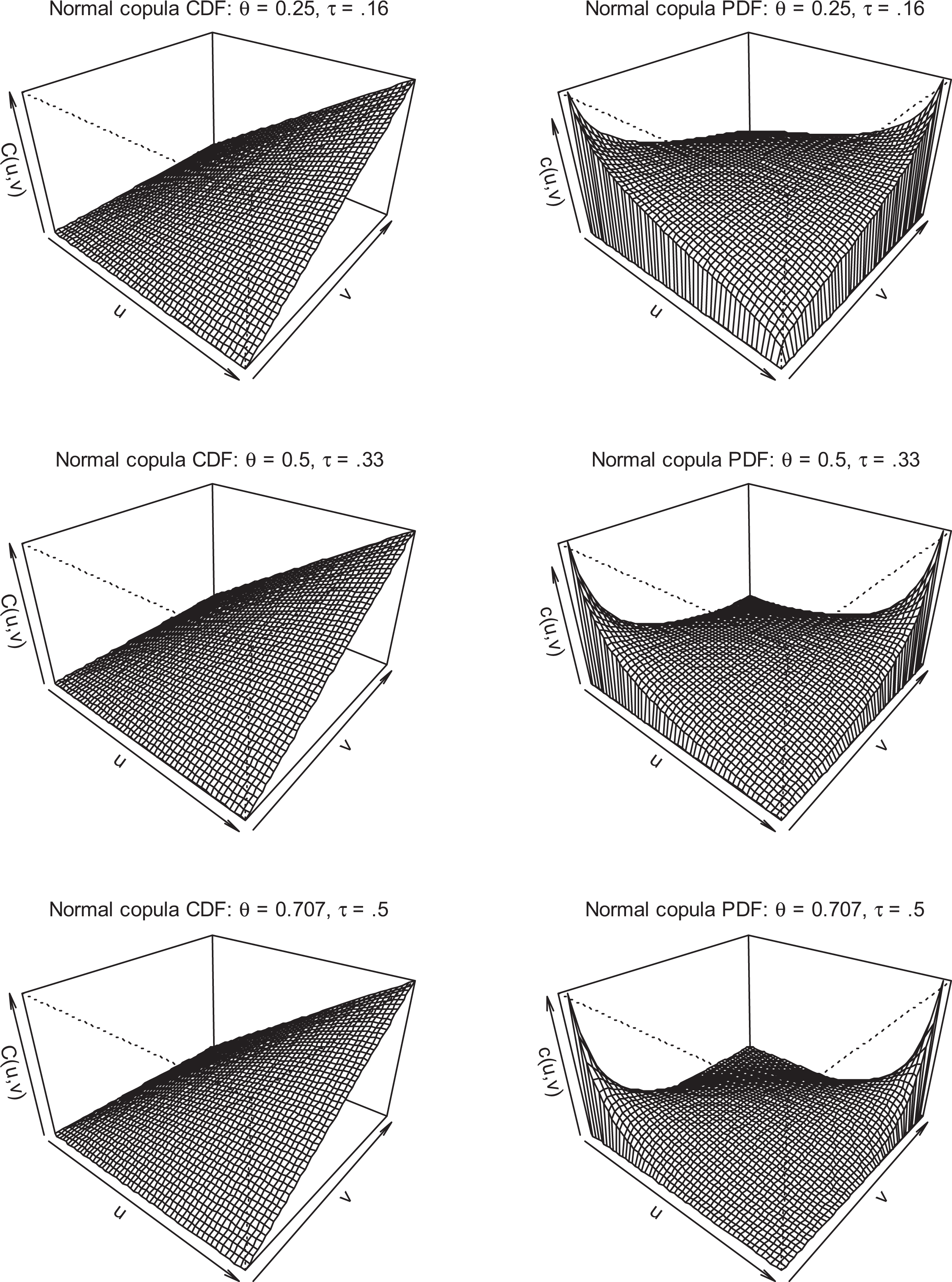
Cumulative distribution function (CDF) and probability density function (PDF) of Normal copula with various association parameters.
The second family of copulas in Table 1 is the Archimedean copulas (Nelsen 2006:109-55). These copulas have a relatively simple form for their construction and, thus, there is a great variety of copulas that fall under the family. A bivariate Archimedean copula is defined as:
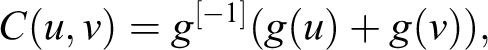
where g [−1] denotes the operation of pseudo-inversion (i.e., equal to zero at zero and the inverse otherwise). As mentioned earlier, plugging a generator function into this formula produces a copula, as shown in Table 1.
Although a great variety of Archimedean copulas have been described in the literature (see Nelsen 2006:116-19), Table 1 depicts four of the most common Archimedean copulas: the product (or independence), Clayton (Clayton 1978; Genest and Rivest 1993), Gumbel–Hougaard (Gumbel 1960; Hougaard 1986), and Frank (Frank 1979; Genest 1987; Nelsen 1986) copulas. Each of the latter three provide instructive examples due to where the weight of the joint probability distribution is most heavy. Figure 2 shows each of these three copulas at the value of their association parameter corresponding to a Kendall’s τ of 0.5. Each copula is quite different in its representation of the dependence structure over the joint distribution. The Clayton copula and Gumbel–Hougaard copula are each most useful for dependence that is high in the lower and upper tails, respectively. On the other hand, the Frank copula allows for both positive and negative association, as well as throughout the distribution where the data are concordant. Although resembling the Normal copula, it is clear that the Frank assigns less probability to the most discordant areas of the distribution for this particular parameter (the exact shape is dependent on the parameter value). As with the example of the Normal copula, increasing or decreasing the association parameter of any of the Archimedean copulas increases the figure’s concordance or discordance, respectively. The product copula is worth noting as a baseline for measuring independence. As the formula in Table 1 shows, the copula does not depend on an association parameter and the Kendall’s τ and Spearman’s ρ are both zero.

Cumulative distribution function (CDF) and probability density function (PDF) of select Archimedean copulas with Kendall’s τ of 0.5.
The final copula family in Table 1 is the Farlie–Gumbel–Morgenstern (FGM) family (Farlie 1960; Gumbel 1958; Morgenstern 1956; Nelsen 2006:77-78). In the table, only a general form for the family is given, as is most typical. FGM copulas can only model weak dependence. Consider the extreme values of the FGM association parameter (−1 and 1) when plugged into the formula for Kendall’s τ in Table 1. The highest and lowest values are for τ are 2/9 and −2/9, respectively. Given that such weak associations can occur in sociological data, the FGM copula is worth noting, though it is not considered in the following examples.
Fitting Copulas
One of the major advantages of copula modeling is in its computational ease relative to other methods of examining joint distributions. Log likelihoods for copulas are easily derived and, thus, standard maximum likelihood procedures are applicable. 4 As for the actual task of computation, the “copula” package (Kojadinovic and Yan 2010; Yan 2007) for the R Statistical Software Environment (R Core Development Team 2011) provides the necessary commands to estimate copula models. All models presented were estimated in R using the “copula” package and other standard commands as described in Yan (2007). The development of this module represents a major step forward in accessibility for those interested in copula models. The package includes, among other things, commands for fitting copula models, drawing random data from a particular copula model with user-defined marginal distributions, and model fit statistics. While the arithmetic for several calculations are shown subsequently, the copula package can compute these values for the user, such as Kendall’s τ, Spearman’s ρ, and joint probabilities.
Several model fit measures are presented. As describe by Joe (2015), we can use the Akaike information criteria (AIC) and Bayesian information criteria (BIC) for model selection, where they are interpreted as penalized log-likelihood functions. They take the typical forms of
Copula Modeling with Sociological Data
Example 1: Known Marginal Distributions and Copula with Simulated Data
In order to gain an understanding of copula models and their application, we first begin with an example with known marginal distributions and a known copula dependency structure connecting them. This example uses randomly generated data meant to resemble the age of death of husbands and wives and the dependency between them, as the “widowhood effect” is a well-established finding in sociology (see, e.g., Elwert and Christakis 2006). Using the copula package in R, margins for each spouse’s age are each fit with the Weibull distribution and a dependency structure from the Gumbel–Hougaard copula. The association parameter for the copula is set to θ = 2, which inserted into the formula for Kendall’s τ in Table 1 produces an association of τ = 0.5. In other words, we are setting the difference in the probability of both marginals being in the same order versus not in the same order at 0.5. For husbands, the Weibull distribution parameters are set to a scale of 65 and a shape of 8. For wives, the Wiebull distribution parameters are set to a scale of 80 and a shape of 8. Figure 3 shows the produced margins with a random draw of N = 1,000. As the figure shows, the scale parameter sets the peak in the age of death and the Weibull distribution assigns much more weight to the older ages, with more skewness to the left. The dependency between them is not apparent just by examining the margins.
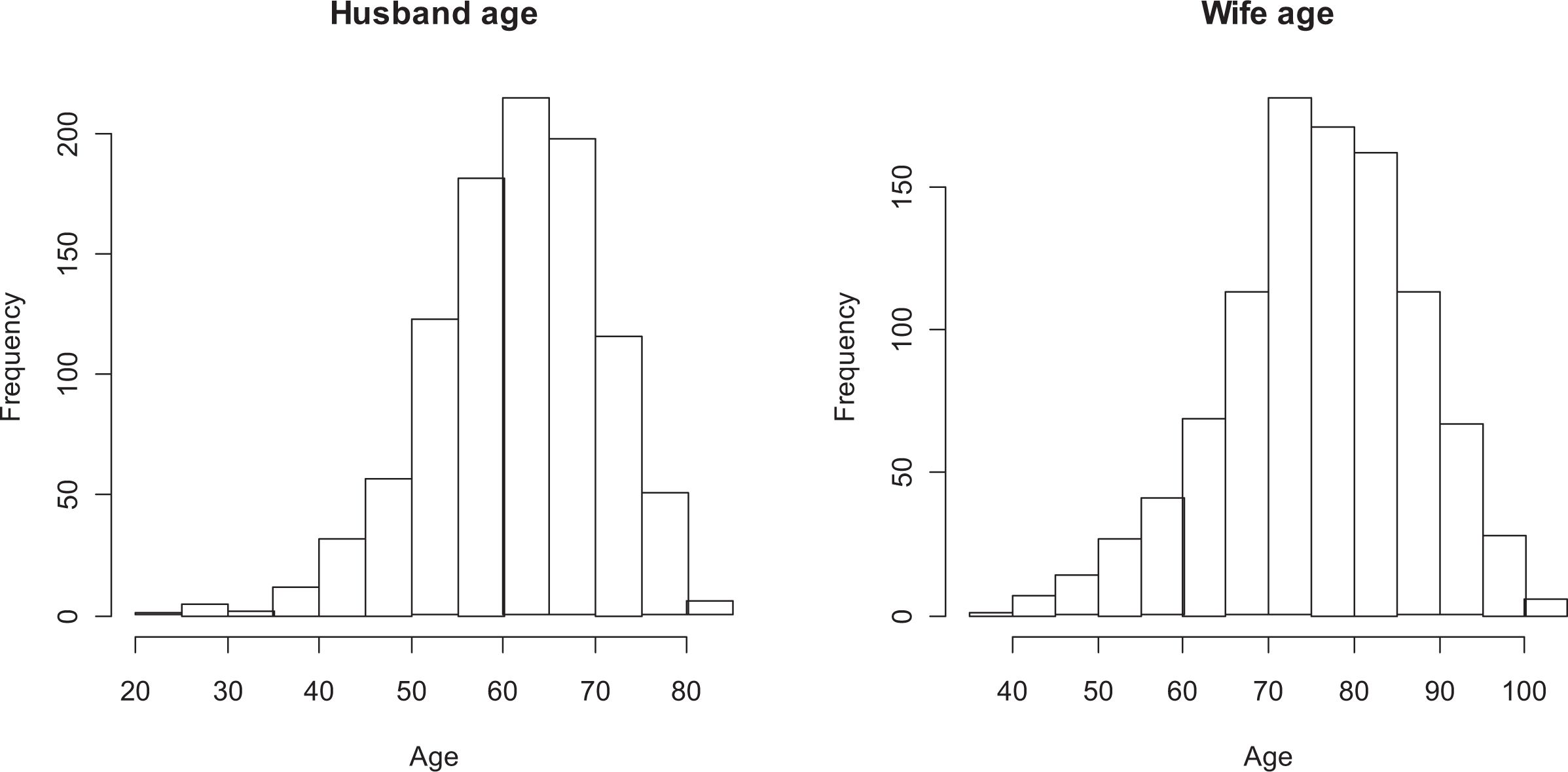
Histograms of randomly generated husband and wife age of death with Weibull marginals and Gumbel–Hougaard copula with association parameter 2.
Yet, the margins are linked by the Gumbel–Hougaard copula and the joint distribution between the margins demonstrates the dependency. Going back to Figure 2, the middle panels depict this exact copula. It was chosen for this example because it assigns high dependency in the upper tail, thus assuming the mortality of spouses is more related as they age. Figure 4 shows how the joint distribution between husband and wives’ age of death changes according to the level of dependency assigned between them (each is a random draw of 1,000). As the parameter is increased, the joint distributions on the left become tighter. As apparent through the contour plots on the right, the dependency is always stronger in older age. That is, spouse’s ages of death are closer when they are older. When a death is experienced at a young age, the surviving spouse is not as likely to die at a similar age compared to the upper part of the marginal distributions. The middle panel of Figure 4 shows the example used of θ = 2.
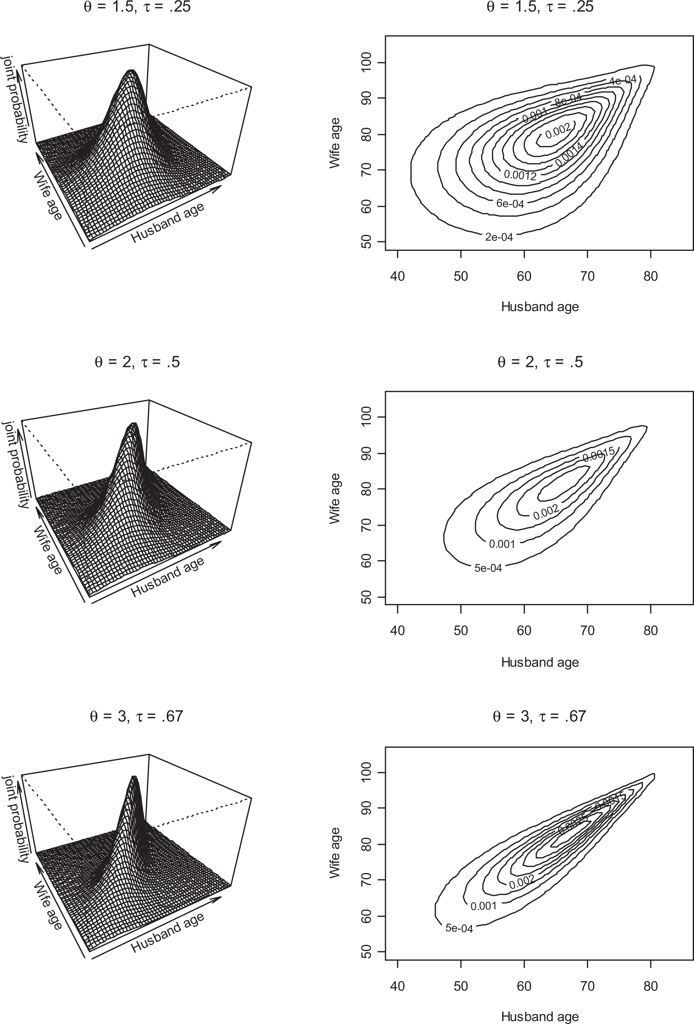
Randomly generated data from Gumbel–Hougaard copulas for various association levels between age of death of husband and wife (each with Weibull marginal distributions).
Demonstrating how copula models allow flexibility in the shape of the dependence structure, Figure 5 gives a comparison of what the joint distribution would look like assuming three alternative copula structures each with the same association of τ = 0.5 (again each with 1,000 random draws). As was described earlier, the Clayton copula exhibits higher dependency in the left portions of marginal distributions, and we can see this in the contour plot and joint probability plot. For spouse’s deaths, this copula is inappropriate if we assume the relationship is stronger when the age of death is older. While the joint distribution from the Frank copula assigns some weight to the higher ages, the distribution is fairly even throughout. Finally, the Normal copula comes the closest, yet still does not exhibit as much dependency in higher ages that we know exists in the data. The fit of various copula models will demonstrate this.
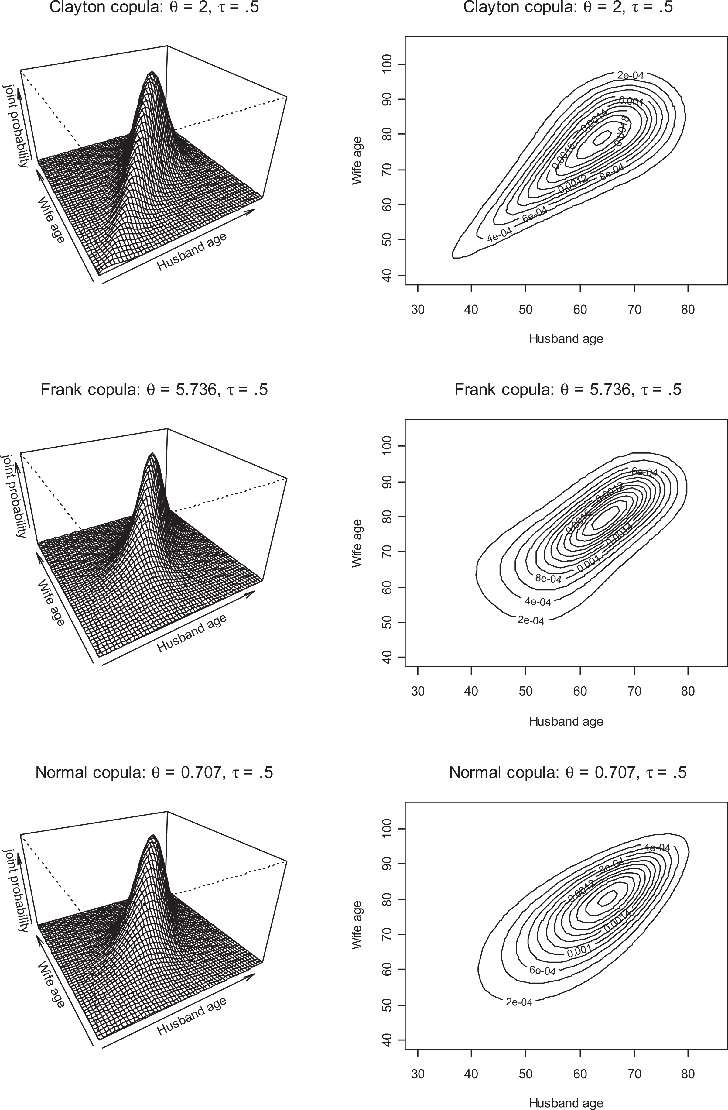
Other potential copula models with association 0.5 for randomly generated age of death of husband and wife (each with Weibull marginal distributions).
As stated earlier, we must properly specify the margins before the copula model is fit. While in this case they are known, it is still instructive to show the example of checking for uniformity. Before this step, a researcher should fit several different feasible marginal distributions to each of those data. Plausible marginal distributions should be garnered from typical examinations of the data, such as histograms, Quantile-Quantile (QQ)-plots, and plots of observed versus predicted values from a distribution. Once a plausible list of marginal distributions is gathered, researchers can then fit those distributions to the margins and use the log likelihood to select the best fitting, through the R command “fitdistr,” for example. Seeing the margins in Figure 3, a researcher may think to fit distributions such as the Weibull, Normal, t, and Cauchy distributions, among others. The values of the log likelihoods (not shown) indicate the best fit is the Weibull, not surprisingly. Since this is a random draw, the shape and scale parameters for the Weibull are not exact. Thus, fitting a Weibull distribution to each marginal separately produces a shape parameter and scale parameter of 8.26 and 64.87, respectively, for the husbands, and 8.23 and 79.54, respectively, for the wives.
The next step is to apply the probability integral transformation to each marginal, such that the values are now that of the CDF and bound on the unit interval. This step is simply a matter of computing the probability for the values of the marginal given the best fitting distribution, akin to determining the complement of a p value (e.g., what is the probability of a wife dying at or below age 60 from a Weibull distribution with a shape of 8.26 and a scale of 64.87?). 5 Figure 6 shows the probability integral transformations. The left side shows the CDF for each marginal. The straight line clearly shows that the CDF is uniform on the unit interval. The histograms on the right also show considerable uniformity across the unit interval.

Probability integral transformation of the marginal distributions of randomly generated husband and wife age of death.
The next step is to fit several different copula models. Table 2 shows each of the discussed Archimedean and elliptical copulas fit to the randomly generated data of spouse’s age of death with the Gumbel–Hougaard association parameter θ = 2 (i.e., τ = 0.5). In each case, the copula parameter is significantly different from zero (p < .001). As shown in Figures 4 and 5, some copulas were more plausible than others. The high RMSE of the independent copula demonstrates that the assumption of no joint relationship has poor fit. Given its weight to dependency at lower values, the Clayton copula is also a particularly poor fit, with the highest AIC, BIC, and RMSE by far and a quite incorrect Kendall’s τ at τ = 0.323. For the other four copulas, the association parameter implies a value of Kendall’s τ close to 0.5. Yet, the AIC, BIC, and RMSE clearly show that the Gumbel–Hougaard copula from which the data were drawn fits best, as the shape of the copula function better captures the dependence across the entire joint distribution. As a point of comparison, Table 3 shows model fits when data are randomly drawn from the same two marginal distributions but with no copula structure specified. Thus, any association is purely random. Indeed, the copula parameters are each closest to the value that translates into a Kendall’s τ of practically zero.
Copula Model Fits to Randomly Generated Husband and Wife Age of Death with Weibull Marginals and Gumbel–Hougaard Copula with Association Parameter 2.
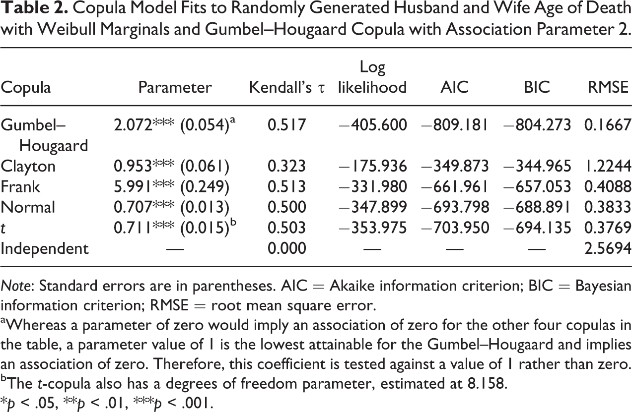
Note: Standard errors are in parentheses. AIC = Akaike information criterion; BIC = Bayesian information criterion; RMSE = root mean square error.
aWhereas a parameter of zero would imply an association of zero for the other four copulas in the table, a parameter value of 1 is the lowest attainable for the Gumbel–Hougaard and implies an association of zero. Therefore, this coefficient is tested against a value of 1 rather than zero.
bThe t-copula also has a degrees of freedom parameter, estimated at 8.158.
*p < .05, **p < .01, ***p < .001.
Copula Model Fits to Randomly Generated Husband and Wife Age of Death with Weibull Marginals and No Dependence Specification.
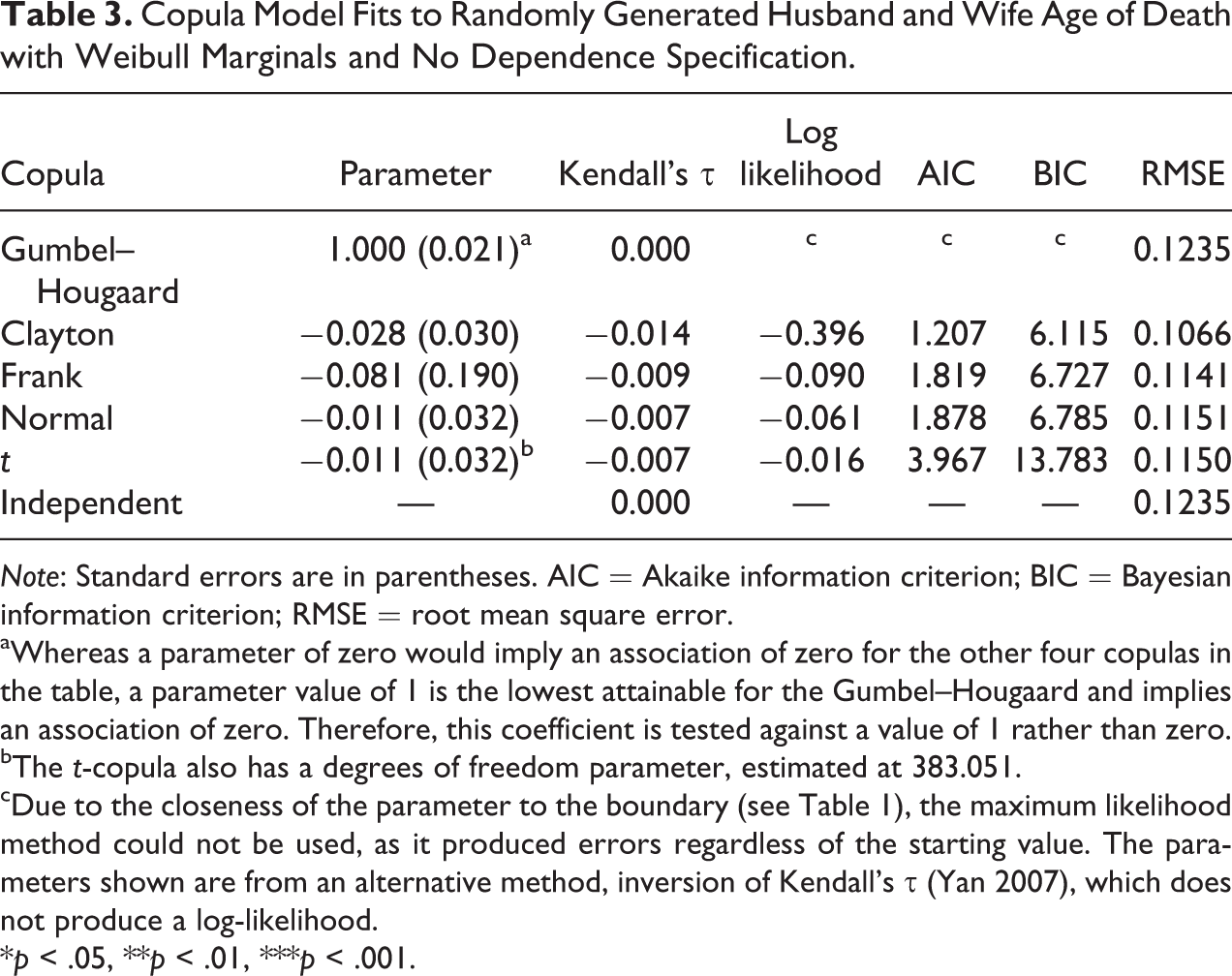
Note: Standard errors are in parentheses. AIC = Akaike information criterion; BIC = Bayesian information criterion; RMSE = root mean square error.
aWhereas a parameter of zero would imply an association of zero for the other four copulas in the table, a parameter value of 1 is the lowest attainable for the Gumbel–Hougaard and implies an association of zero. Therefore, this coefficient is tested against a value of 1 rather than zero.
bThe t-copula also has a degrees of freedom parameter, estimated at 383.051.
cDue to the closeness of the parameter to the boundary (see Table 1), the maximum likelihood method could not be used, as it produced errors regardless of the starting value. The parameters shown are from an alternative method, inversion of Kendall’s τ (Yan 2007), which does not produce a log-likelihood.
*p < .05, **p < .01, ***p < .001.
Next, we can calculate probabilities by plugging values into the copula function given in Table 1. Recall that by the definition of a distribution function and the copula:

First then, an examination of the marginal probabilities is in order. Here, F 1 and F 2 are the Weibull distributions defined earlier. Taking the mean from the simulated data as an example, we find that a wife or husband that dies at the respective means of 75.29 and 61.84 each have a value of about u = v = 0.461 on the marginal CDFs (i.e., 46.1 percent of wives and husbands die at or below those ages). To find the joint probability for a couple both dying at or below those respective means, we can plug the values into the Gumbel–Hougaard distribution given in Table 1 (or simply use the “pCopula” function in R):
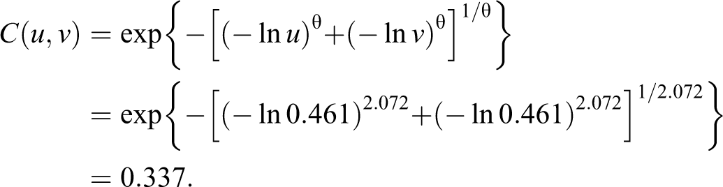
Thus, given an association of τ = 0.511, 33.9 percent of couples have both members die at or below the mean on each marginal distribution. If we change the husband’s age of death to 45, that individual now has a value of 0.054 on the marginal distribution function, while the couple is located at 0.049 on the joint cumulative distribution. That is, most couples survive to a higher combination of ages. Finally, keeping the husband at the mean but changing the wife’s age of death to 90, we compute a wife-specific cumulative distribution value of 0.928 and a couple joint probability of 0.459. Of course, this example is one of known distributions and dependency. Thus, we move on to an example with empirical data.
Example 2: Time Series in the Margins with Empirical Data
Arguably, the most common application of copula models is that of understanding the relationship between various time series. In finance in particular, a common goal is to model dependencies between stocks or other financial instruments in order to create a portfolio with decreased risk. In this case, copula models can provide the dependence between the time series in manner that is not a function of the distribution of the margins. Thus, in the margins, we can model the time series in a manner that accounts for autocorrelation (i.e., association of the current value with past values) and heteroskedasticity of both series separately. In this example, we examine a classic sociological outcome, suicide (for a review, see Wray, Colen, and Pescosolido 2011), in a simple bivariate time series example. The relationship between the monthly suicide rate per 100,000 and unemployment rate from January 1999 to December 2011 is examined. The suicide rate comes from mortality data from the Centers from Disease Control and Prevention. Unemployment data come from the Bureau of Labor Statistics, with the seasonally unadjusted rate used since such seasonal fluctuations occur in suicide as well and we are interested in their association. Figure 7 presents both series. If we take these data as the objects of analysis, the Pearson’s correlation is 0.624 (p < .001).

Time series plot of monthly unemployment rate and suicide rate.
In this example, we are interested in the dependence between unemployment and suicide, but we have reason to hypothesize that there is both an autoregressive (AR) and seasonal (SAR) component to each rate. In time series analysis, the goal is to model the dependence of current values on past values in order to remove any time trend. Differencing the data, such that the current value is the change from the previous year (also called a return), is also typical in order to satisfy the time series model assumption of stationarity (i.e., the effect of past values on the current value is constant across time). Once an appropriate model is selected, the residuals become the object of analysis, as these provide data that are stationary and devoid of a time trend (for more on time series modeling, see Shumway and Stoffer 2011). Analyses of both series demonstrated that the best fitting AR model had a lag of two and an SAR component for the 12 month cycle, and was differenced to account for stationarity. For unemployment, AR(1) = 0.13 (p > .05), AR(2) = 0.27 (p < .001), and SAR(12) = 0.83 (p < .001). For suicide, AR(1) = −0.57 (p < .001), AR(2) = −0.31 (p < .001), and SAR(12) = 0.84 (p < .001).
As with the previous example, the first step to copula modeling is to calculate the probability integral transformation and check the uniformity of the marginal CDFs. As with any linear regression, the residuals from an AR model are assumed normal with mean zero and some variance. Thus, we fit the normal distribution respectively to both series of residuals. As expected, the fitted mean for both is essentially zero (unemployment: mean = 0.00098, variance = 0.04357; suicide: mean = 0.00007, variance = 0.00096). Then, these distributions are used to compute the respective complements of the p values for each marginal. Figure 8 demonstrates that both marginals appear to satisfy the uniformity assumption.

Probability integral transformation of residuals from autoregressive (AR) model.
As mentioned earlier, it is wise to fit many possible copula models when applied to empirical data (Trivedi and Zimmer 2007). Thus, each of the elliptical and Archimedean copulas was fit to the marginal distributions, with the results shown in Table 4. Although the Frank copula fits the data best according to each of the model fit statistics, all the copulas lead to the same conclusion: We cannot reject the null hypothesis that the association between unemployment and the suicide rate is zero. The linear correlation reported earlier would lead to the conclusion that the shared variance between unemployment and suicide is 39.0 percent. Once the margins are modeled appropriately in a manner that accounts for autocorrelation and a measure of dependence taken that is free from influence of the marginal distributions, the square of Spearman’s ρ from the best fitting Frank copula results in a shared variance of only 0.9 percent. According to Kendall’s τ, the difference between the probability of suicide and unemployment being in the same order is only −0.064 greater than being in a different order. Indeed, the 95 percent confidence interval (CI) computed from the standard error of the association parameter overlaps zero for both measures of association (Kendall’s τ: [−0.163, 0.037]; Spearman’s ρ: [−0.242, 0.056]). Figure 9 shows the contour plot of the joint distribution for the fitted Frank copula. As the neat, elliptical shape demonstrates, there is virtually no relationship throughout the distribution (cf. Figures 3 and 4).
Copula Model Fits to Unemployment Rate and Suicide Rate Time Series.

Note: Standard errors are in parentheses. AIC = Akaike information criterion; BIC = Bayesian information criterion; RMSE = root mean square error.
aWhereas a parameter of zero would imply an association of zero for the other four copulas in the table, a parameter value of 1 is the lowest attainable for the Gumbel–Hougaard and implies an association of zero. Therefore, this coefficient is tested against a value of 1 rather than zero.
bThe t-copula also has a degrees of freedom parameter, estimated at 155.005.
cDue to the closeness of the parameter to the boundary (see Table 1), the maximum likelihood method could not be used, as it produced errors regardless of the starting value. The parameters shown are from an alternative method, inversion of Kendall’s τ (Yan 2007), which does not produce a log likelihood.
*p < .05, **p < .01, ***p < .001.

Contour plot for fitted joint distribution of unemployment and suicide rates.
This example demonstrates the utility of copula models for time series data. In particular, the method enables the researcher to take into account autocorrelation in both variables of interest prior to fitting the dependence. For sociologists, such modeling has further applications. For example, a researcher could use the method to verify whether two different measures of the same phenomenon are associated as expected. In this vein, the method could assess whether the United States’ two measures of crime, the Uniform Crime Report and National Crime Victimization Survey, are indeed moving in unison as might be expected, a long-standing question for those who study crime (Biderman and Lynch 1991; Lynch and Addington 2007). Of course, the preceding model was not meant as the definitive analysis of suicide and unemployment, but was merely used to provide an example. Instead, researchers would most likely be interested in a more detailed analysis, such as including covariates in the margins, to which we now turn.
Example 3: Copula with Predictors from Empirical Data
Here, we consider the relationship of education and alcohol use, modeled with several predictors in the margin (see, e.g., Crosnoe and Reigle-Crumb 2007). The data come from the NLSY97. The NLSY97 is an annual nationally representative survey of youth who were aged 12–17 in 1997. A subset of the 1998 cross-sectional survey that includes only those aged 17 at the time of the survey is analyzed for a sample size of N = 1,298. The outcomes of interest are GPA and a count response to, “During the last 30 days, on how many days did you have one or more drinks of an alcoholic beverage?” GPA is measured on the traditional 0–4 range and comes from the students’ school transcripts. 6 Several predictor variables are included in the modeling of these two marginal distributions. Indicator variables are included for gender, community type (urban vs. rural), and whether any paid work was reported. A series of dummy variables also measure race (white, black, and Hispanic) and household (HH) parental structure (both biological parents, other two parent, single parent, and other structure). Finally, total HH income is reported by the parent of the respondent and logged due to skewness. 7
In this particular example, there is reason to believe that either GPA or alcohol use could affect the other. Yet, we are still interested in their association and would like to control for other potential influences for both variables. More importantly, commonly used measures of association are inappropriate to understand the relationship between a continuous, potentially skewed measure and a count variable. The assumptions behind linear correlation are not met, despite such relationships appearing often in both correlation tables and regression analyses. This scenario is one in which copula models are useful.
Unlike the preceding examples, we are interested in including covariates in the margin. While the NLSY97 is expansive in scope such that many predictors could have been tested, for simplicity, only a small group of predictors is included in the models and these are kept the same for both margins. Thus, sociologists should consider all the model selection, model fit, and model diagnostics techniques that are typically employed when fitting each of the margins separately, and the predictors need not be the same. 8 Here, care is still taken in modeling the margins in a manner that satisfies the uniformity assumption demonstrated in the previous sections via an appropriate regression model.
The first step is to appropriately model the margins and confirm their uniformity. Beginning with GPA, Figure 10 depicts a histogram, which shows some degree of skew. An ordinary least squares (OLS) regression was fit with each of the predictors described earlier (not shown). We then use the probability integral transformation to compute the CDF, which again is akin to computing p values on the appropriate distribution. Given that this is OLS regression, we use the normal distribution function to compute the probability of each respondent’s observed value on the cumulative distribution of GPA using the model variance and their respondent-specific fitted value as the mean. Figure 11 attests to the importance of fitting the marginal distribution correctly. The top panel shows the probability integral transformation of an OLS regression with GPA in its original scale, while the bottom panel shows an OLS regression of GPA with the Box–Cox transformation for normality of the residuals applied with a best fitting power of 1.7 (Box and Cox 1964). Clearly, the former is not uniform on the unit interval, while the latter is. 9 Given the assumption of uniformity, the transformation of GPA is used in the copula model.
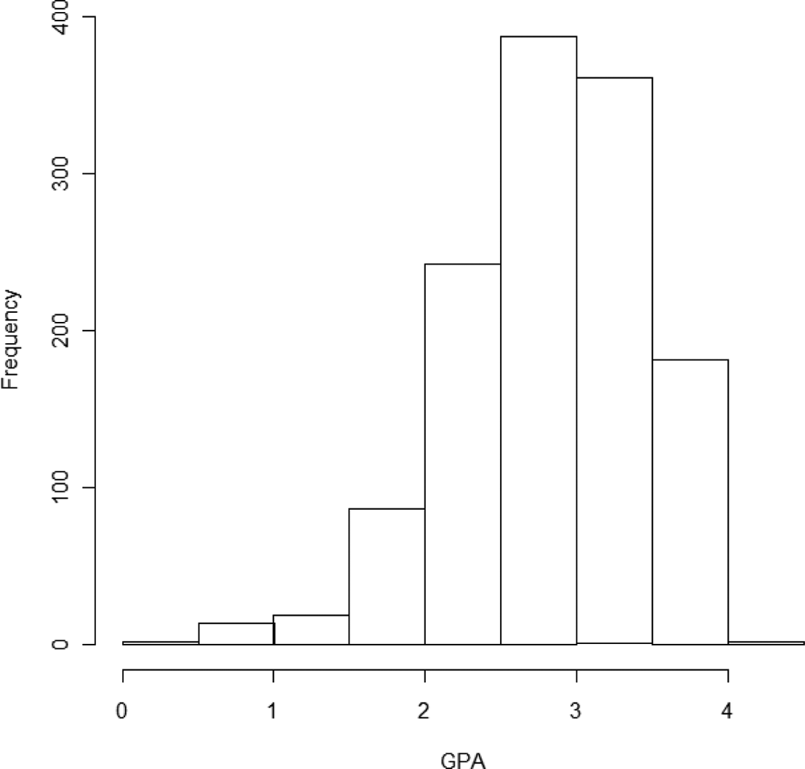
Histogram of grade point average (GPA; National Longitudinal Survey of Youth 1997 [NLSY97]).

Probability integral transformation from ordinary least squares (OLS) regression models for grade point average (GPA; National Longitudinal Survey of Youth 1997 [NLSY97]).
A different generalized linear model was then applied to the count of days using alcohol. Given the nature of this count measure, a Poisson or negative binomial regression is most appropriate, with the latter used given the presence of overdispersion (mean = 1.91; variance = 17.8). Here for the probability integral transformation, we compute the complement of the p values associated with the respondent’s observed alcohol use from the negative binomial distribution using the model dispersion and the exponentiated respondent-specific fitted value (so that it is in the correct units) as the mean, shown in Figure 12. The figure depicts uniformity, though the range is not the unit interval. From the above mentioned definition, the copula is still unique on the range of the distribution function as long as it is uniform (i.e., jumps do not appear). In these particular data, no obvious horizontal plateaus appear, there are virtually no ties across the margins, and the models presented subsequently converge. Given several cautions regarding discrete data in the margins, these assumptions should always be checked carefully. 10
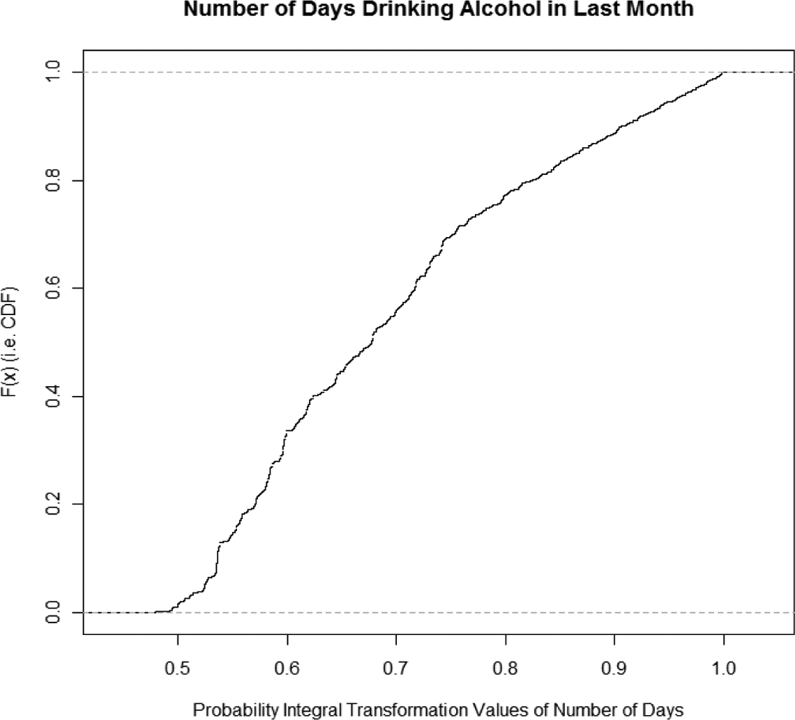
Probability integral transformation from negative binomial regression models for number of days drinking alcohol in last month (National Longitudinal Survey of Youth 1997 [NLSY97]).
Once the researcher is certain that they have correctly modeled the margins and that they satisfy these assumptions for discrete data, he or she can use the values of the regression coefficients as starting values for estimating a copula model. That is, the copula parameter and each of the regression coefficients, as well as any other model parameters such as the residual standard error in the OLS regression and the overdispersion parameter in the negative binomial regression, are estimated simultaneously via maximum likelihood. 11 Table 5 shows the best fitting model for each of the elliptical (Normal) and Archimedean (Frank) families, as well as the Product/Independence copula as a point of comparison. Both a model χ2 test and the significance of the copula parameter provide evidence to reject the null hypothesis that GPA and days drinking alcohol are not associated, controlling for the predictors in the model. Beginning with the former, a likelihood ratio test between the Independence copula model and either the Normal copula (χ2 = 30.607, df = 1, p < .001) or Frank copula (χ2 = 23.712, df = 1, p < .001) demonstrate that the model with an association parameter is a better fit. The AIC and BIC suggest that the Normal copula (AIC = 8,189.59, BIC = 8,308.46) is the better model relative to the Frank copula (AIC = 8,196.48, BIC = 8,315.36), and the RMSE is lower for the Normal.
Copula Models for GPA and Number of Days Drinking Alcohol in Last Month (NLSY97).
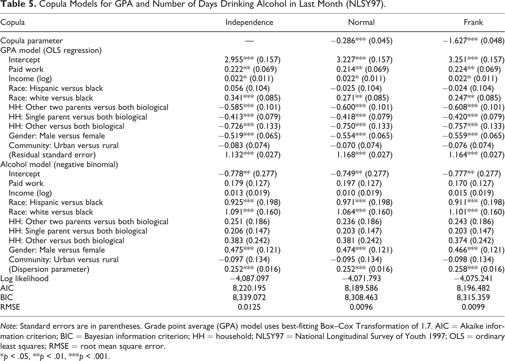
Note: Standard errors are in parentheses. Grade point average (GPA) model uses best-fitting Box–Cox Transformation of 1.7. AIC = Akaike information criterion; BIC = Bayesian information criterion; HH = household; NLSY97 = National Longitudinal Survey of Youth 1997; OLS = ordinary least squares; RMSE = root mean square error.
*p < .05, **p < .01, ***p < .001.
Thus, we can use the copula parameter from the Normal model to determine the association between GPA and days drinking alcohol. The association parameter is θ = −0.286. We use the formulas from Table 1 to compute either of the nonparametric measures of association. As described earlier, the linear correlation can only capture the dependence free of influence from the marginal distribution in the case of a Normal copula and Normal margins. Kendall’s τ and Spearman’s ρ, however, have the advantage of making no assumption about the distribution of either marginal or the relationship between them (Schweizer and Wolff 1981) and providing the association after controlling for important predictors of both phenomena. Spearman’s ρ is −0.274 (
Although the strength of the association is not remarkably different between linear correlation and the other two measures of association, there is a further advantage of the copula modeling procedure. Namely, the dependence varies over the joint distribution, as opposed to a similar effect of a one unit increase in the case of linear correlation or even a linear model. Figure 13 shows the fitted copula probability distribution for the estimated parameter. A PP plot confirms a good fit between the empirical copula and the fitted copula with this association, as depicted in Figure 14. Thus, we are able to model a more detailed joint relationship, and the results make intuitive sense. Given the negative association, the highest probability is in the discordant sections, such that GPA and alcohol use have higher discordant dependency at high and low values of each. In the middle of the distribution, alcohol use and GPA are not as strongly associated. As the nonzero weight in the opposite corners show, even possible concordance is not completely discounted, though albeit rare by comparison. The various shapes of the copula models presented, together with the association parameter, allow for a variety of dependencies.

Parametric normal copula fit from National Longitudinal Survey of Youth 1997 [NLSY97] copula models.

Probability–probability (PP) plot of [NLSY97] empirical and fitted copula.
The importance of the ability to control for predictors in the margins becomes further apparent when examining probabilities, as one’s place in the joint distribution is no longer determined solely by values on the two outcomes of interest, but also on the values of the predictors. Within the margins, we see that higher GPA is predicted by paid work, higher income, white race, female gender, and living with both biological parents (relative to all other HH structures). Higher number of days drinking alcohol is predicted by white and Hispanic race (relative to black), and male gender. 13 For given values of the predictors and outcomes, we can then compute the joint probability of GPA and alcohol use. The first step is to compute the associated complement of the p value on the CDF given those values, using the normal for GPA and negative binomial for alcohol use with the estimated model variance and dispersion, respectively. As with the simulated example, these values are then inserted into the best-fitting copula to determine the joint cumulative probability.
A few examples will demonstrate this computation. 14 If we assume a white, urban, working female teen from a HH with both biological parents and an income of US$68,971, this individual has a predicted mean of 1.71 days drinking and 3.68 GPA. Now suppose that individual has an observed value of 2 days drinking and a GPA of 4.00. Using the model dispersion and variance parameters, respectively, and the respondent-specific predicted means, these observed values translate to a value on the respective marginal CDFs of 0.798 for drinking and 0.933 for GPA conditional upon the covariates. To compute the joint cumulative probability, we use the best-fitting Normal copula formula in Table 1:

That is, the joint probability of having a lower GPA and drinking fewer times given the values on the covariates is 0.736. Supposing instead a Hispanic, urban, nonworking female teen from a HH with both biological parents and an income of US$10,615 and observed days drinking of 0 and GPA 3.6, this individual lies at 0.645 for the drinking marginal distribution function, 0.872 for the GPA marginal distribution function, and 0.541 on the joint distribution function. Finally, for a white, rural, nonworking male teen from a HH with both biological parents and income of US$19,029 and observed days drinking of 1 and GPA 1.41, they lie on the 0.673 for drinking, 0.025 for GPA, and only 1.0 percent of 17-year-olds are at or lower on the joint distribution of drinking and GPA given the observed covariates.
While the association parameter was taken as the object of interest in this example, sociologists may also use the copula method with a focus on the covariates. In such a scenario, the joint probability between two variables might be considered a nuisance parameter that needs to be controlled to garner more accurate covariate estimates. In the aforementioned example, we might be hesitant to include alcohol use as a predictor of GPA because we are unsure this is the correct temporal order, yet still wish to account for the relationship. One approach to such a scenario is structural equation modeling. For noncontinuous variables, however, structural equation modeling requires computationally intensive methods such as generalized latent variable models (see, e.g., Skrondal and Rabe-Hesketh 2005). Instead, we could fit a copula model that accounts for the dependence (with or without covariates for alcohol use), with flexibility in the margins and computational advantages from the maximum likelihood and simultaneous estimation.
Other Applications
While this introductory article to copulas prohibits a detailed discussion of every aspect of the methodology, it is worth noting several applications not demonstrated earlier that are potentially quite useful to sociologists. First, any copula can be rewritten in a survival function form, connecting the joint survival function to its univariate margins in a manner completely analogous to the coupling in a copula (Nelsen 2006:32-34). In applications, researchers may be interested in the probability of surviving beyond a particular point, rather than the probability of surviving until that point, a case where the survival copula is appropriate. In the above mentioned simulated example of spousal ages of death, it is easy to see how the survival copula is useful, and we could redo the exercise with the survival version of the Weibull distribution. With empirical data, issues arise in survival analysis, such as censoring, that are still applicable and researchers should consult methods to deal with such concerns (see Hougaard 2000; Shemyakin and Youn 2006).
Second, copulas are particularly adept at modeling “tail dependence,” or associations of relatively rare, but related events or values occurring in the tails of each of the margins. In examining some of the copulas in the above mentioned figures, I alluded to the various copulas’ ability to model joint behavior in the tails. We can explicitly compute the nonparametric tail dependence parameters (denoted λ
L
and λ
U
for lower and upper), which are interpreted as the limiting value of one marginal surpassing a particular value on the marginal distribution function given that the other marginal is already greater than that same value (McNeil et al. 2005; Nelsen 2006:214-16; Trivedi and Zimmer 2007:25-26). Some copulas are better suited for modeling tail dependence, such that researchers should carefully choose which copulas to model depending on whether joint rare values are of interest and where they are expected to occur. In Figure 2, we saw that the Clayton and Gumbel–Hougaard were useful for modeling relationships in the lower and upper tail, respectively. The upper and lower tail dependence parameters are
Third, while this introduction focused exclusively on the bivariate case, copulas are theoretically extendable to higher dimensions. That is, Sklar’s Theorem in n-dimensions (Nelsen 2006:46-47) is:

We can extend the other formulas mentioned earlier as well to the multidimensional case, though at high enough dimensions, the current ability to easily estimate the models is hampered. Frees and Valdez (2008) and Zimmer and Trivedi (2006) provide excellent examples of three-dimensional applications. In the NLSY97 analysis, we could, for example, add a depression scale to the copula, furthering past research on GPA, depression, and drinking (see, e.g., Shippee and Owens 2011). The ability to model the margins separately allows researchers a very flexible method to understand the association between phenomena in ways that might prove difficult otherwise, including relationships between rare events, mixed effects models, and highly skewed data.
Discussion
Copulas provide a flexible methodology for understanding associations between related phenomena and their joint probabilities. Thus, copula models ask a fundamentally different question than typical techniques modeling conditional values. Rather than how does variable X influence variable Y, copulas ask: how do two variables move together in unison and how strong is that concurrent movement at various point in the distribution? The substantive outcome of interest then becomes the joint probability of two particular values of each marginal distribution occurring together, and the association is the hypothesis tested, while allowing for considerable flexibility in the modeling of each marginal. The copula function “couples” two univariate marginal distributions together in a way that preserves the margins and provides a measure of dependence that does not require the specification of an a priori joint distribution. Instead, the probability integral transform is used to convert the margins to a uniform distribution, whose joint relationship is then modeled via a copula function. It is often difficult to define, and even more difficult to estimate, joint distributions for margins in situations where one or more of the margins are nonnormal. This approach allows for consideration of a plethora of marginal distributions in a maximum likelihood estimation setting and numerous shapes of joint distributions that capture different strengths of local dependence.
Three examples were provided to demonstrate the method. The first included randomly generated data meant to simulate the joint distribution of spousal mortality. The value of this example was to provide a short introduction to the basics of the method. The real benefit for sociologists no doubt lies in approaches similar to the latter two examples using empirical data. In the first example, time series models were used to adjust for autocorrelation and stationarity to model the joint distribution of suicide and unemployment. In the second example of 17-year-old’s GPA and days using alcohol, the modeling procedure showed how copulas can be used to understand the association and joint distribution between two nonnormal variables, while at the same time controlling for important predictors for each. While this example shares similarities with structural equation modeling, the flexibility in the margins opens possibilities that go beyond what is feasible in structural equation modeling. With models similar to the given examples, as well as the other avenues described in the previous section, the applications within sociology are numerous, as we are often confronted with nonnormal data whose joint relationship we seek to understand.
To close, it is worth noting that any method can produce erroneous results when not properly applied. Copulas are no exception to this rule, and their misuse as a cause of the Great Recession (through violated statistical assumptions and use of a particular distribution on data to which it did not appropriately fit) has actually been well documented through qualitative sociological studies of financial market employees (MacKenzie 2011) and quantitative economic studies of the models used leading up to the financial crisis (Brigo, Pallavicini, and Torresetti 2010; Donnelly and Embrechts 2010; Zimmer 2012). Thus, sociologists should exercise caution and safeguard that each marginal distribution, as well as the copula used to bind them, is fit using the most appropriate method and best-fitting model. Several additional cautions were given throughout where sociologists should take care, such as in the case of discrete marginal distributions or in using copula models with the correct assumption of tail dependence (see Hays and Kachi 2009 for other instances). Further, there are alternative methods for creating or assessing bivariate distributions and associations that researchers might consider, such as seemingly unrelated regression, inversion methods, and mixture models. MacKenzie’s (2011) findings concerning copulas and the sociology of knowledge can be applied much more broadly, as any method can seemingly take hold as the “correct” method such that it becomes unquestioned for a period. His qualitative study reminds those conducting quantitative analysis to take great care in checking the assumptions of one’s models. While copulas, like any method, can be abused, the goal of this article was to help sociologists take the first step toward using them correctly within our discipline.
Footnotes
Acknowledgments
I am grateful to Ken Ferraro and Sarah Mustillo for their valuable feedback on this manuscript. I would also like to thank Brian Kelly, Michael Light, Chris Uggen, Scott Feld, and Joy Kadowaki for input on various aspects of the paper, as well as Arkady Shemyakin and John Dodson of the School of Mathematics at the University of Minnesota who introduced me to the method in their classes.
Declaration of Conflicting Interests
The author(s) declared no potential conflicts of interest with respect to the research, authorship, and/or publication of this article.
Funding
The author(s) received no financial support for the research, authorship, and/or publication of this article.