
Abstract
Loglinear smoothing (LLS) estimates the latent trait distribution while making fewer assumptions about its form and maintaining parsimony, thus leading to more precise item response theory (IRT) item parameter estimates than standard marginal maximum likelihood (MML). This article provides the expectation-maximization algorithm for MML estimation with LLS embedded and compares LLS to other latent trait distribution specifications, a fixed normal distribution, and the empirical histogram solution, in terms of IRT item parameter recovery. Simulation study results using a 3-parameter logistic model reveal that LLS models matching four or five moments are optimal in most cases. Examples with empirical data compare LLS to these approaches as well as Ramsay-curve IRT.
Keywords
Unidimensional item response theory (IRT; Lord & Novick, 1968) models play an important role in present-day educational measurement and testing. With marginal maximum likelihood (MML) estimation of IRT item parameters (Bock & Aitkin, 1981; Bock & Lieberman, 1970), the IRT model is expanded to include a latent trait distribution, denoted here by
Flexibility in model specification for
Generally, parsimony is a major consideration in statistical modeling. It is especially important in psychometrics with the usage of relatively more complex models such as the unidimensional 3-parameter logistic (3PL) IRT model, multidimensional IRT models, and cognitive diagnostic models. These models involve many estimable parameters and are typically associated with identifiability issues (Haberman, 2005). Therefore, flexible yet parsimonious options for estimation should be considered in these cases, as the ideal model for
The most common fixed specification for
The focus of this article is a semiparametric model for
Other smoothing methods, including LLS, have been used for discrete latent trait and mixture IRT models by Rost and von Davier (1992, 1995), von Davier (2005), and Xu and von Davier (2008). Although these smoothing approaches have been around for quite some time, they were implemented in the context of complex multidimensional discrete latent trait modeling (see, e.g., mdltm software; von Davier, 2005). Furthermore, the algorithms used for estimation of
In the next sections, we review MML estimation of item parameters and provide an overview of the various methods for characterizing
Characterization of the Latent Trait Distribution in MML Estimation
MML estimation provides estimates of item parameters by assuming that the item response data are obtained from a random sample from a population of latent traits with a certain distribution. With MML, the likelihood is expanded to include
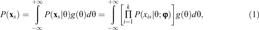

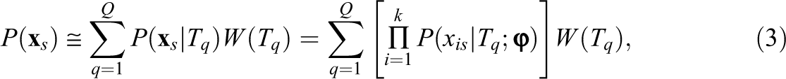
Bock and Lieberman (1970) introduced MML estimation using Gauss–Hermite quadrature to approximate integrals involving the normal distribution (see Stroud & Secrest, 1966). Quadrature utilizes values of a function at a finite set of discrete points to approximate the full area under the curve. A quadrature weight,
To approximate the integral in Equation 1, quadrature is used as given by,

The EH Method for g(θ)
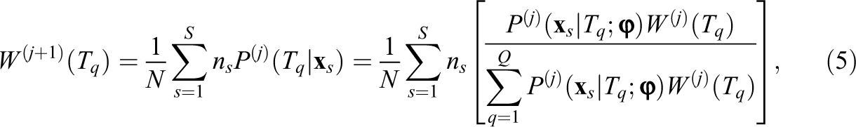
Since θ is unobserved and therefore considered missing, Bock and Aitkin (1981) used the EM algorithm (Dempster, Laird, & Rubin, 1977) to implement MML estimation of item parameters. In the E-step, expectations of sufficient statistics Nq (the expected number of examinees at Tq) and Riq (the expected number of examinees at Tq responding correctly to item i) are computed so that item parameters may be estimated in the M-step. In the M-step, estimates of the item parameters are computed that maximize the expected log likelihood from the E-step. These estimates are then used as updated quantities to compute the expectations in the next E-step, and so on, until convergence.
The EH method for
These

Equation 6 gives the quantity that is to be maximized with the EH method. It is apparent from Equation 6 how the item parameters and the distributional parameters are simultaneously estimated. The starting values,
Other Approaches to Specify g(θ)
There are a variety of alternative methods to specify a nonnormal latent trait distribution, none of which have gained enough popularity to replace the EH approach as the most widely used. Xu and Jia (2011) used a parametric approach by estimating parameters of the skew-normal distribution in MML (mean, variance, and skewness). Thissen’s Johnson curve approach estimates Johnson curve parameters (Johnson, 1949) along with item parameters in MML yielding curves with different combinations of skewness and kurtosis (available in MULTILOG 7.0 software; Thissen, 2003; van den Oord, 2005).
Another approach to estimating
Ramsay-curve IRT (RC-IRT; Woods & Thissen, 2006) implements MML estimation by using a splines-based approach to estimate a smooth
Loglinear Smoothing
Holland and Thayer (1987, 2000) introduced LLS as a method for reducing irregularities in discrete observed test score distributions. LLS estimates probabilities for discrete distributions based on an unsaturated loglinear model, and therefore, only some properties of the observed frequency distribution are preserved by fitting M moments. This section discusses LLS models for observed and latent distributions.
Model Features and Specification for Observed Distributions
Let
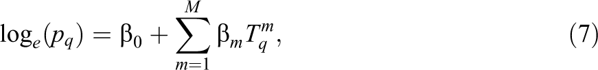
where
The main feature of LLS is that it matches sample moments of the observed distribution. The maximum likelihood estimates from the model in Equation 7,

that is, the sample moments of
LLS for the Latent Trait Distribution
The LLS model for latent distributions is the same as Equation (7); however the values of
Consider the number of parameters estimated for
Choosing M and Q
The more complex the distribution represented by the
In terms of choosing Q, generally, the larger the value of Q, the finer the characterized distribution, or the more closely the estimated distribution will approximate a continuous distribution. It may be inferred that the more points specified for the discrete distribution, the better the approximation to g(θ) and thus better MLEs for the item parameters. Therefore, it is desirable to have a large Q in order to capture the complexities in the distribution, but the benefit may taper. The maximal number of discrete points needed when estimating both points and weights of g(θ) has been discussed for the Rasch model—it was found that approximately Q = k/2 is sufficient (De Leeuw & Verhelst, 1986; Lindsay, Clogg, & Grego, 1991). Tzamourani and Knott (2002) found in tests with k ranging from 3 to 21 that the 2PL model needs fewer than Q = k/2. Importantly, Tzamourani and Knott (2002) also showed in an empirical example that item parameter estimates resulting from varying levels of Q do not differ by much, and discrimination parameter estimates get smaller as Q decreased. They note that this effect on the discrimination parameter estimates is likely a function of coarsening the scale upon which the slope can be appropriately estimated—it is more challenging to discriminate examinees across fewer points or when they are categorized into fewer ability levels.
Note that with LLS, we estimate only M parameters in addition to item parameters, and therefore, the value of Q has no influence on parsimony. In other words, we may choose a relatively larger value of Q to characterize a fine version of
The EM Algorithm With LLS
To implement LLS for
M(aximization) Step: Stage 1
For each item separately, solve the maximum likelihood equations given in Equations 9, 10, and 11, using the expected counts
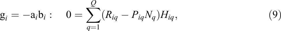
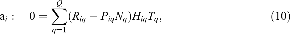
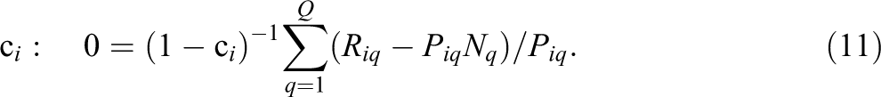
Here,
M(aximization) Step: Stage 2
Begin a Newton cycle either by using a set of starting values for Compute a vector of fitted frequencies defined by:
Compute an estimated variance–covariance matrix for this vector defined by Using a singular value decomposition, solve for Compute a new vector of coefficients With the estimates Use the maximum absolute difference between the elements of the original
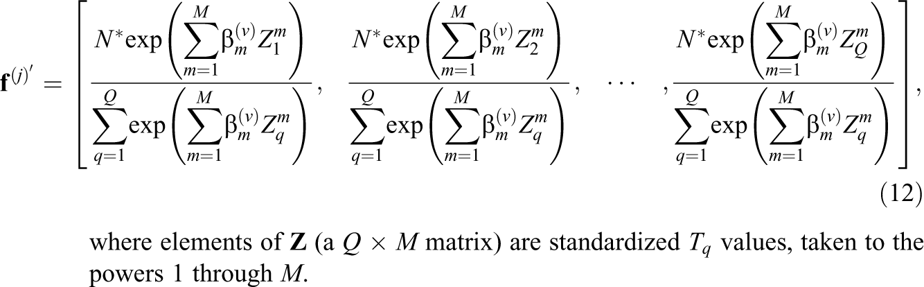
The final output of the M-step is an updated value for the fitted frequencies, which appear as the final quadrature weights,
The software LLSEM 1.0 (LogLinear Smoothing Expectation Maximization) implements these algorithms (Casabianca & Lewis, 2011b). LLSEM is capable of item parameter estimation under the 1PL, 2PL, and 3PL dichotomous IRT models using the normal distribution assumption, the EH method, and LLS. In our implementation of LLS, we keep the quadrature points equally spaced and fixed throughout the entire estimation procedure to identify the scale (Lewis, 1985; see the Appendix for more information on this identification method). Furthermore, there is no standardizing during the iterations, unlike what occurs in many commercial software programs. Instead, we scale item parameter estimates after convergence to the scale of the estimated latent trait distribution. Thus, the mean and SD of the resulting distribution are not necessarily 0 and 1, respectively, as would be the result in many commercial software programs. More information on LLSEM is available in the Appendix.
Simulation Study Design
To provide an evaluation of LLS’s utility for item parameter recovery, we conducted a Monte Carlo simulation study for IRT item parameter estimation and compared LLS to the fixed normal model and the EH method.
1
We varied skewness and number of modes of the true
Item Response Generation Conditions
Fifty item responses were generated for 1,000 simulated examinees from each of the following true latent trait distributions, each with mean and variance equal to 0 and 1, respectively: (a) standard Normal density, N(0,1); (b) negatively skewed continuous distribution with a skewness of −1.5, created using a mixture of two normal distributions (

True population latent trait distributions.
Item responses were simulated using calibrated 3PL items from a 2008 National Mathematics Assessment (Item parameters were provided by ETS; Copyright (C) 2011 ETS. www.ets.org). The distribution of the difficulty parameters was approximately normal (symmetric) but centered around .2. The mean a parameter was 1.13 (SD = 0.25), mean b parameter was 0.21 (SD = 0.51), and mean c parameter was 0.16 (SD = 0.05).
Calibration Conditions
Each data set was calibrated in LLSEM with the following specifications for
The levels of M were specified in a nesting structure according to Q. For all levels of Q, LLS models matching M = 2, 3, 4, and 5 moments were fit. These levels were chosen for two reasons. First, what the first few moments can capture can be hypothesized and conceptualized, higher moments probably cannot. Second, based on work with observed test score distributions, it has been noted that at least four or five moments are typically needed to adequately characterize a univariate distribution (Holland & Thayer, 2000). Beyond the five-moment model, M varied with Q in such a way that there was not an excessive number of conditions, but to include enough levels that questions regarding the effect of moment matching on item parameter recovery could be addressed. We aimed to find the optimal point in the bias–variance trade-off. We fitted the 10-moment model for
Outcome Measures
Item parameters are the sole focus of this simulation study. We compared item parameter estimates to the true item parameters using bias and root mean square error (RMSE) criteria. We computed the average RMSE using the square root of the average mean square error across the 50 items. We also used a multivariate measure of error to assess overall recovery of item parameters called the mxD as used by Woods (2008). Specifically, this measure is the absolute difference between the item characteristic curve (ICC) using estimated item parameters and the ICC using the true item parameters, computed for each item across the Q quadrature points. Within condition, item, and replication, the maximum of these absolute differences (over the Q quadrature points) was determined. The mean of the absolute maximum difference was taken across the 50 items, and the mean was also taken across replications.
Simulation Study Results
Normal g(θ)
There was very little error in the normal case to start with! The mxD values for the LLS models (0.044–0.046) were the same as the EH results (0.045–0.046; see Table 1 for these mxD values). Differences between LLS models (across values of M) were negligible, and there was no pattern of increasing or decreasing as a function of the number of moments. There was no difference between Q = 31 and Q = 61, since virtually all model specifications yielded the same amount of error, on average. However, for Q = 11, the average RMSE with the fixed normal distribution specification was 0.01 higher than all other conditions. This difference appeared when examining differences in average RMSEs for the individual item parameters. That is, compared to the Q = 31 and Q = 61 conditions, the Q = 11 condition yielded about 0.03 higher average RMSE for the a and b parameters when using a fixed normal distribution for
Maximum Absolute Difference (mxD) in Item Characteristic Curves (Estimated vs. True)

Note. Normal = fixed (standard) normal distribution assumption; LLS = loglinear smoothing; EH = empirical histogram method.
Negatively Skewed g(θ)
For the negatively skewed
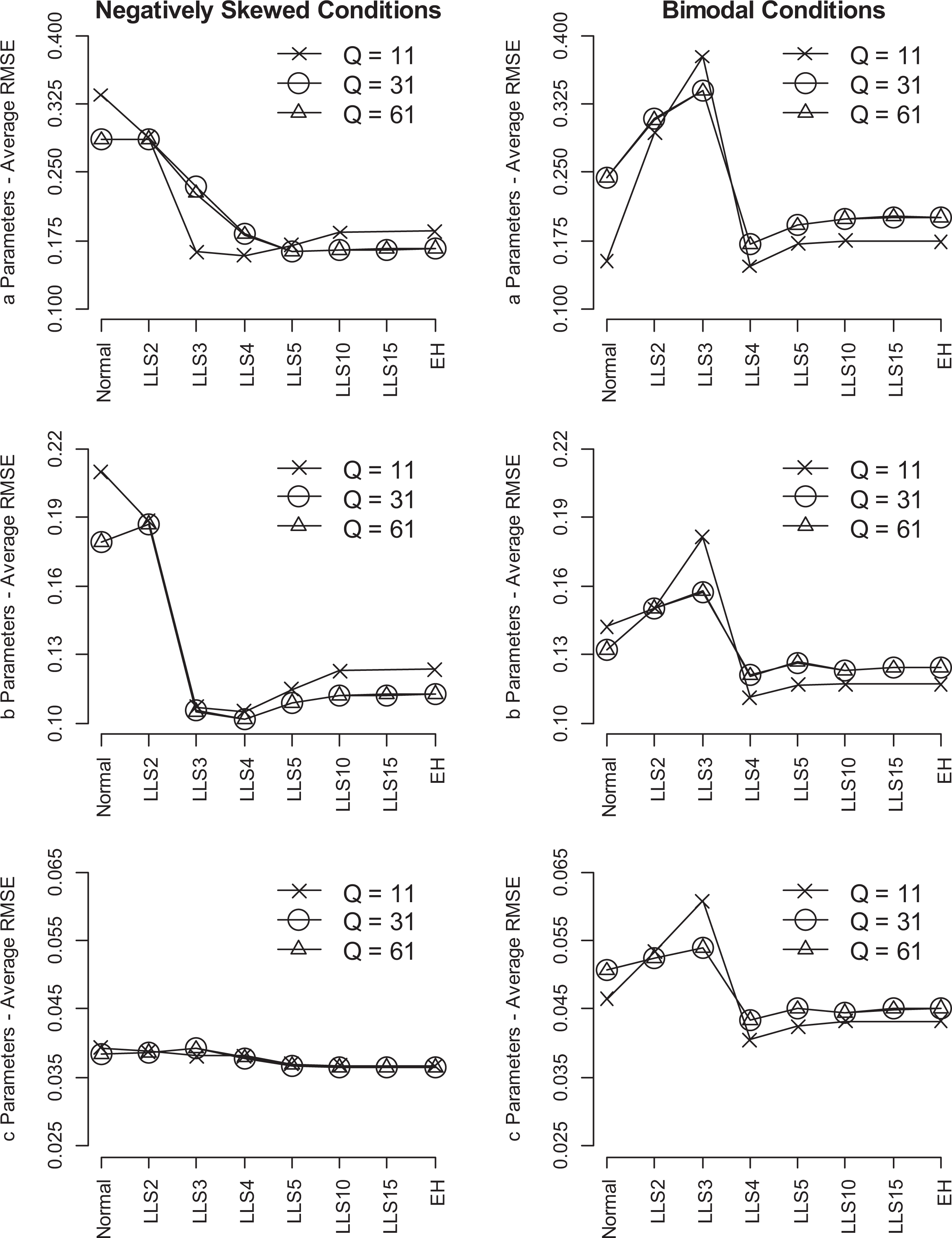
Average root mean square error plots for a, b, and c item parameter estimates for negatively skewed and bimodal g(θ) conditions. The left column of plots is for the negatively skewed conditions and the right column for the bimodal conditions.
Figure 2 provides profile plots per parameter estimate and for the true negatively skewed (left column of plots) and bimodal (right column of plots) latent trait distributions. These plots show the trajectory for error for the three different Q levels, as we increase in model complexity. Here, × is Q = 11, О is Q = 31, and Δ is Q = 61. We excluded the profile plots for the true normal
There was no difference between Q = 31 and 61. However, when Q = 11, the fixed normal distribution assumption yielded a mxD of 0.089, which is higher than mxD = 0.046 yielded by LLS4. This difference is reflected in Figure 2 in the a and b parameters. Under LLS3, the Q = 31/61 conditions yielded larger average RMSEs than Q = 11 for a parameters. For both the a and b parameters, the average RMSEs were slightly larger for the Q = 11 condition under LLS5.
The left column of plots in Figure 3 depict item-level bias for the negatively skewed condition for the a, b, and c parameters (going down the column) under the fixed normal assumption, EH, and LLS4 with Q = 31. For brevity, only LLS4 was shown here (in filled circles) because it has been shown throughout the results to be the top performer. LLS4 yielded consistent positive bias across the a parameter scale with fluctuations around 0. EH and especially the fixed normal model showed a downward bias as a increased. Bias in the b parameters was usually smaller with LLS4 than the other models—this was especially true at the ends of the scale. In a couple of instances, the LLS4 model yielded approximately 0 bias, while EH yielded about 0.1 (in both the positive and negative directions). All three models had similar levels and trends for bias for the c parameter: positive bias for lower c parameters and negative bias for higher c parameters. LLS4 had relatively smaller biases with higher c parameters, although the highest true c in this simulation was only .25.
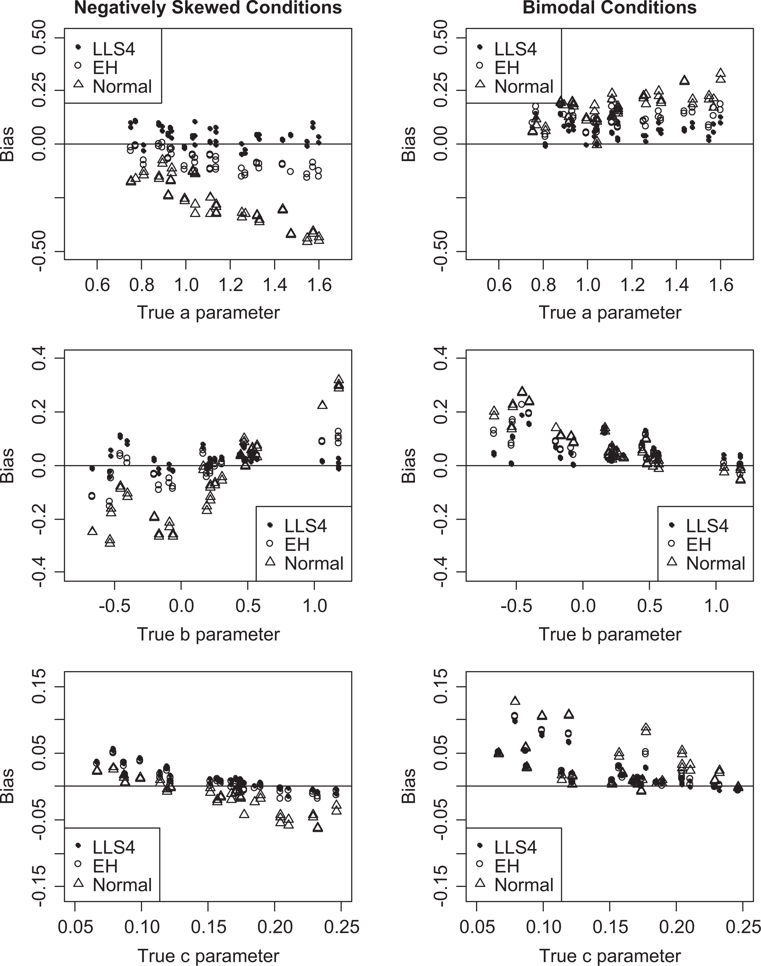
Item bias plotted as a function of true item parameters for 50 items in simulation study under the normal, EH method, and four-moment loglinear smoothing (LLS) models when Q = 31. The top, middle, and bottom rows show the bias for the a, b, and c parameters, respectively. The left column of plots is for the negatively skewed conditions and the right column for the bimodal conditions. LLS4 = four-moment LLS model; EH = empirical histogram; Normal = fixed normal distribution assumption.
Bimodal g(θ)
For the bimodal condition, the mxD ranged from 0.045 to 0.078 when Q = 11 and 0.050 to 0.072 when Q = 31/61. The absolute least error was obtained with Q = 11 under LLS4 (mxD = 0.045). All LLS models performed similar to EH except for LLS2 and LLS3, which yielded more error. Although differences between the models were minimal, the mxD and the average RMSEs for LLS4 were always smaller (mxD difference = 0.003) than the EH results.
All three types of item parameters also showed the smallest average RMSEs under LLS4 (see Figure 2). There was an increase in error between LLS2 and LLS3 and then a large decrease in error between LLS3 and LLS4. After
Differences between levels of Q were not straightforward. The two higher levels of Q were identical and there were inconsistent differences between Q = 11 and Q = 31/61. For example, for all models but the LLS3 model, mxD was smaller when Q = 11. Conversely, for LLS3, mxD was larger when Q = 11. This is also shown on the profile plots (Figure 2) for each of the item parameters.
The right column of Figure 3 shows item-level bias plots for the bimodal condition. In the top plot, the bias for the a parameters increases with the true a value for the fixed normal distribution assumption and EH, but this trend was not true for LLS4. Instead, bias tended to be smaller under LLS4. For the lower b parameters (between −0.7 and 0), the LLS4 model yielded smaller (positive) bias than the other models. Toward the center of the b scale, the three models converged. Larger positive bias was found for the smaller c parameters (0.07 to 0.18), and LLS4 yielded the smallest of these biases. As c increased, bias for all models converged around 0.
Empirical Illustration Using the PISA Mathematics Assessment—Shanghai Sample
The PISA is an international study conducted by the Organization for Economic Cooperation and Development that assesses 15-year-old students in mathematics, reading, and science. Shanghai-China outperformed all other countries in all three PISA subject assessments in 2012. We analyzed 11 dichotomously scored mathematics items from a subset (n = 1,623) of the Shanghai-China sample (n = 5,177) to demonstrate the 2PL EM algorithm with LLS for
In our RCLOG specifications, we set the SD for the multivariate normal prior on the spline coefficients to 500 for maximal flexibility in the shape of the distribution. We fitted all possible RC-IRT models with order up to 6 and number of breaks up to 6 and selected the best fitting model based on the consideration of several criteria as described in Woods (2006a). The criteria are the log-likelihood LogL, the Akaike information criterion (AIC; Akaike, 1973), the Bayesian information criterion (BIC; Schwarz, 1978), the Hannan–Quinn criterion (HQ; Hannan, 1987), and the Kolmogorov–Smirnov test for normality (KS; Kolmogorov, 1933; Smirnov, 1939). The models with the smallest values of the LogL, AIC, BIC, and HQ signal the best fit. Woods (2006a) notes that it is common for these various criteria to yield different models; however, the current analysis revealed consistency across three of these four indices. That is, the 3-2 model was selected by BIC, HQ, and AIC. The LogL selected the 6-6 model. Both of these models are significantly different from normal model by the KS test. We proceed with the comparison of models using results from 3-2 RC-IRT model solution.
Figure 4 provides the latent trait distributions from the MML estimation of item parameters for the PISA items. 3 The thicker solid curve is the discretized normal distribution. The thinner curves are distributions from EH, LLS, and RC-IRT, all of which should capture varying degrees of nonnormality, if any nonnormality should exist. Indeed, the estimated latent distributions all exhibit moderate positive kurtosis and moderate negative skewness. (For reference, consider statistics for the 3-2 RC: M = 0.000, SD = 1.001, skewness = −.884, kurtosis = 4.004.) While they all share similar shapes, the RC 3-2 and EH distributions are more leptokurtic than the LLS distributions. These distributions indicate a population of examinees that tend to perform relatively higher on the latent trait scale, which is expected from the Shanghai-China sample.
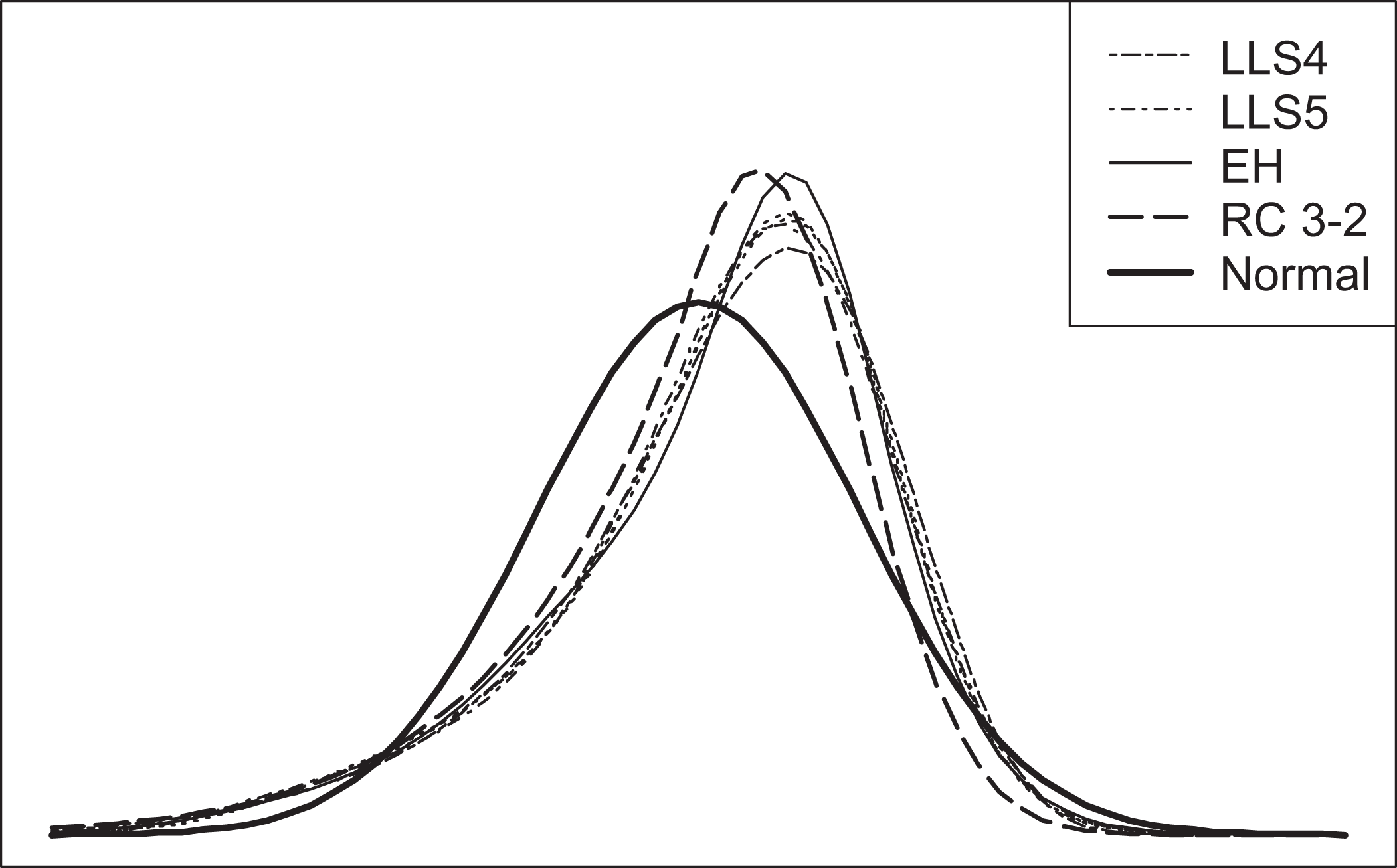
Estimated latent trait distributions with Q = 61 from Programme for International Student Assessment mathematics data (Shanghai-China sample). LLS4 = four-moment LLS model; LLS5 = five-moment loglinear smoothing (LLS) model; EH = empirical histogram method; RC 3-2 = 3-2 Ramsay-curve item response theory solution; Normal = fixed normal distribution assumption.
The profile plots of the a and b item parameter estimates from the PISA analysis in Figure 5 provide a visual depiction of the differences between estimates by method for g(θ). The x-axes on these plots arrange items sorted ascending by the normal parameter estimate. When examining the top plot of Figure 5, we see that all methods with the exception of the normal model yield very similar a parameter estimates. Only with the most discriminating item (#5) was there a difference between RC-IRT and the other methods. In this case, RC-IRT yielded a marginally higher estimate (2.28 vs. ∼2.16 for the other methods). Note that although we observed a slight difference in the distributions for EH/RC-IRT and LLS solutions, the item parameters here are basically equivalent. There were inconsistent differences between the normal model estimates (black line and diamond symbol) and the other methods, in that for some items, the normal estimate was higher and for other items lower. This may be related to the corresponding difficulty estimates for these items (see the bottom plot of Figure 5). For easy items, the normal model yielded larger b estimates compared to the other methods.
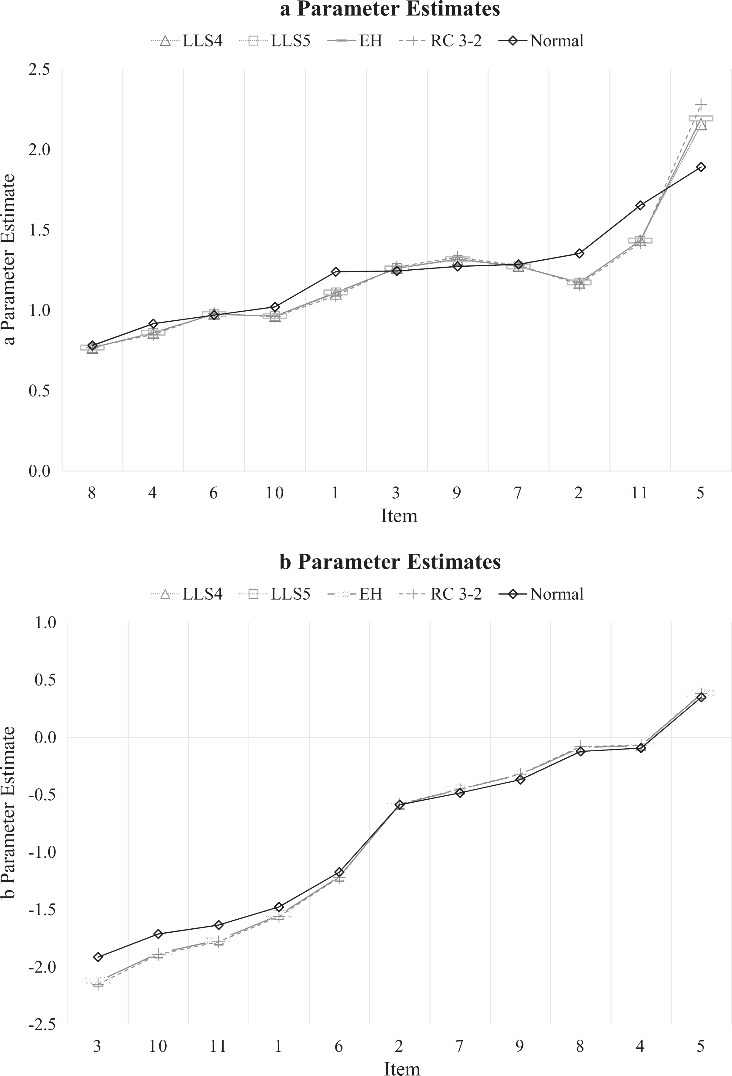
Item response theory (IRT) parameter estimates plotted in profiles by method for g(θ) for 11 mathematics items from the 2012 Programme for International Student Assessment, Shanghai-China sample. The a and b estimates appear in the top and bottom plots, respectively. Items are sorted in ascending order by the normal parameter estimate. LLS4 = four-moment loglinear smoothing (LLS) model; LLS5 = five-moment LLS model; EH = empirical histogram method; RC 3-2 = 3-2 Ramsay-curve IRT solution; Normal = fixed normal distribution assumption.
Although the LLS4 and EH models were very similar in parameter recovery as per the simulation results, it was technically the LLS4 model that yielded the most accurate ICC, when g(θ) was nonnormal (shown via the MxD statistic in Table 1). The EH MxDs were always larger but by a very small order. It is reasonable to cautiously consider the LLS4 estimates here the best of the normal, EH, and LLS models. However, we must remind you that the distributions in the simulations and in this example differ, and the IRT models differ, making a direct correspondence between this example and the simulations less than straightforward.
Empirical Illustration Using the MOCI
We used data from an administration of the MOCI (Hodgson & Rachman, 1977) to a sample of undergraduates enrolled in an introductory psychology class at the University of North Carolina (n = 1,080) to provide an additional demonstration of LLS. The MOCI is a multidimensional true/false measure of obsessive–compulsive symptoms. In this illustration, we use 9 items from the MOCI which together are unidimensional and comprise the “wash” subscale (Woods, 2002). The subscale includes items such as “My hands do not feel dirty after touching money.” True responses to these items indicate a lack of obsession/compulsion with washing, and therefore, respondents with negative latent trait values have higher levels of obsession and compulsion and the opposite is true as
Figure 6 shows the series of distributions all with some degree of positive skew and kurtosis (3-2 RC: M = 0.000, SD = 1.002, skewness = 0.729, kurtosis = 3.801). The deviations from normality are clear when comparing these to the normal distribution. Interestingly, the EH distribution exhibits a very small secondary mode on the right side—the other methods did not reveal this. It is true that at some point, LLS would also show this same mode, but it is unknown with what value of M. Aside from that difference found in the EH distribution, all other estimated distributions share the same shape.

Estimated latent trait distributions with Q = 61 from Maudsley Obsessional Compulsive Inventory wash item data. LLS4 = four-moment LLS model; LLS5 = five-moment LLS model; EH = empirical histogram method; RC 3-2 = 3-2 Ramsay-curve item response theory (IRT) solution; RC 2-4 = 2-4 Ramsay-curve IRT solution; Normal = fixed normal distribution assumption.
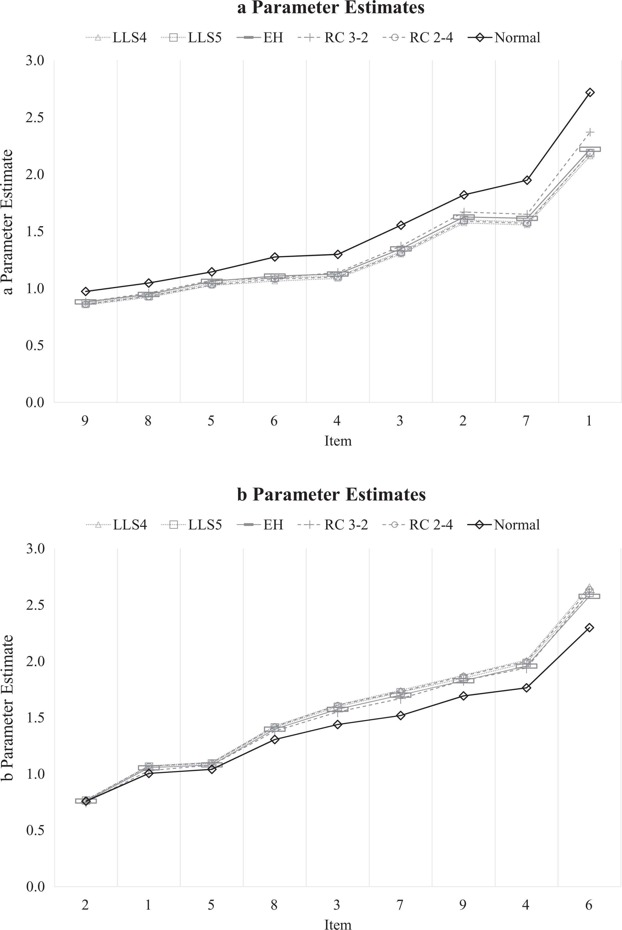
Item response theory (IRT) parameter estimates plotted in profiles by method for g(θ) for 9 wash items from Maudsley Obsessional Compulsive Inventory. The a and b estimates appear in the top and bottom plots, respectively. Items are sorted in ascending order by normal parameter estimate. LLS4 = four-moment LLS model; LLS5 = five-moment LLS model; EH = empirical histogram method; RC 3-2 = 3-2 Ramsay-curve IRT solution; RC 2-4 = 2-4 Ramsay-curve IRT solution; Normal = fixed normal distribution assumption.
Figure 7 reveals only small differences between item parameters yielded by the models estimating
Differences between the normal model item parameter estimates and estimates from the other methods for
Discussion
Our goals were to provide the LLS/EM algorithm for IRT item parameter estimation, evaluate its effectiveness when
It was generally true that somewhere along the
While there was virtually no difference in item parameter recovery for Q = 31 and Q = 61, there were some effects to the discrimination parameter between Q = 11 and the higher Q conditions. Using more points to represent the distribution (keeping the range of the distribution fixed) should impact the estimation of the slope. That is, more points characterize a finer
The data examples provide a comparison of item parameters and latent distributions generated by a series of methods including RC-IRT for two data sets which both involved distributions with moderate skewness and kurtosis. The simulation and real data results were consistent: with the exception of the normal model, differences between models for g(θ) were mostly minor. We did observe many similarities between LLS and EH in both data sets, but we know from simulations that smoothing results in more accurate item parameter estimates.
LLS Versus Other Methods for g(θ)
It is obvious why any nonparametric or semiparametric approach for g(θ) may be preferred over the fixed normal model—these models will properly model deviations from normality in the characterization of g(θ) thereby yielding more precise item parameter estimates. The problematic part about the flexibility of the most popular nonparametric approach, the EH approach, is that it involves an estimation procedure requiring possibly many additional parameters. For long tests and for complex models, where many item parameters are being estimated, this may lead to estimation and identifiability issues (Haberman, 2005). LLS offers a unique advantage over the EH method by estimating only the M moments necessary to capture nonnormality, making the LLS solution more parsimonious. We showed in our simulations that in addition to improvements in parsimony, LLS actually yields better item parameter estimates in terms of RMSEs and MxDs. However, we must remind the reader that this result is strictly applicable to the data under study.
The payoff for using LLS is potentially great. For example, suppose we have a 50-item test to be calibrated with the 3PL with Q = 61. Under the normal model, only 150 parameters are estimated. However, under EH, we estimate 150 + 60 = 210 parameters. With a five-moment LLS model, we can obtain the same or better item parameter estimates with 150 + 5 = 155 parameters estimated. The number of additional parameters involved with RC-IRT is equal to the sum of the order and number of breaks minus two. Therefore, for the 3-2 model that was selected for our two empirical examples, we estimated an additional 3 + 2 – 2 = 3 spline coefficients. For the most complex RC-IRT model, we would estimate 6 + 6 – 2 = 10 spline coefficients.
RC-IRT is a very flexible option. The RCs estimated and selected for analysis in our empirical examples appear almost identical to the curves from the EH and LLS methods and the resulting item parameter estimates were very similar to these methods as well. The major difference between RC-IRT and LLS is in the implementation. With RC-IRT, the analyst considers a variety of candidate RC curves based on spline functions with different combinations of order and number of breaks and selects a model based on a series of model fit indices. There is also a decision to be made in regard to the SD of the multivariate prior distribution. Consequently, there are many possible solutions depending on the final SD chosen as well as the model selected based on the multiple fit indices, which often select different models. In our opinion, the wide range of options makes RC-IRT less straightforward than LLS.
Further, because it is a splines-based approach, RC-IRT has the potential for indeterminacy. The estimation procedure depends on the number and location of breaks in the RC used to characterize g(θ). There is an upper limit on the number of breaks available in RCLOG (2–6 breaks). This dependency may result in estimation issues if there are insufficient breaks or if the breaks appear in inopportune locations. For example, Woods and Thissen (2006) reported issues with convergence because the estimated curve required more quadrature range than was available.
LLS provides smoothed solutions based on a moment-matching procedure that relaxes the potentially overfitted g(θ) generated by EH. It does this all while yielding the same or better item parameters with less of an expense in terms of the number of estimated parameters. The EH is a special case of the LLS framework (when M = Q – 1). The mathematics/statistics underlying LLS is accessible to researchers and analysts and the approach to implementing LLS is straightforward with minimal consideration of anything but moments. Considering that as little as four moments can recover adequately a bimodal distribution, using LLS is very simple with minimal decisions to be made that would otherwise generate inconsistencies in model selection. LLS would not present many indeterminacy issues like RC-IRT because it can easily be implemented with very large Q values to characterize g(θ).
Suggestions for Use and Final Remarks
One model that kept reappearing as the best in terms of yielding smaller average RMSEs is the four-moment LLS model. Clearly, the two- and three-moment models are generally insufficient. We suggest the four- or even the five-moment models for the future use of LLS to estimate
There are some caveats that should be noted in the interpretation of the simulation results. First, there is limited generalizability because we explored only two distinct nonnormal latent trait distributions. Further, the different item parameters in the 3PL IRT model will have different levels of robustness to poor characterizations of the latent trait distribution. For example, if the scale is not wide enough (range restriction) or if there is improper representation of the distribution, then there may be problems estimating the a parameter. Also, it is known that there are issues estimating c parameters, and the estimation of the a and c parameters are interdependent as the c defines the lower asymptote for the ICC. Future research will implement LLS in other contexts such as multiple group
Footnotes
Acknowledgment
The authors are extremely grateful to Brian Junker and three anonymous reviewers for their careful reading and useful feedback on this research and article. We are also grateful to Carol Woods for providing the MOCI data and for assisting us with the RCLOG software.
Authors’ Note
A version of this article was presented at the 2012 National Council on Measurement in Education annual meeting.
Declaration of Conflicting Interests
The author(s) declared no potential conflicts of interest with respect to the research, authorship, and/or publication of this article.
Funding
The author(s) disclosed receipt of the following financial support for the research, authorship, and/or publication of this article. This research is based on the first author’s dissertation carried out at Fordham University and was jointly supported by Fordham University’s Distinguished Dissertation Research Fellowship (2009) and by Educational Testing Service’s (ETS) Harold Gulliksen Psychometric Research Fellowship (2009). The research reported here was also supported in part by the Institute of Education Sciences, U.S. Department of Education, through Grant R305B1000012 to Carnegie Mellon University. The opinions expressed are those of the authors and do not represent views of the Institute or the U.S. Department of Education, Fordham University, or ETS.