Size Matters

Abstract

Since the 1970s, catalogs of protest events have been at the heart of research on social movements. To measure how protest changes over time or varies across space, sociologists usually count the frequency of events, as either the dependent variable or a key independent variable. An alternative is to count the number of participants in protest. This article investigates demonstrations, strikes, and riots. Their size distributions manifest enormous variation. Most events are small, but a few large events contribute the majority of protesters. When events are aggregated by year or by city, the correlation between total participation and event frequency is low or modest. The choice of how to quantify protest is therefore vital; findings from one measure are unlikely to apply to another. The fact that the bulk of participation comes from large events has positive implications for the compilation of event catalogs. Rather than worrying about the underreporting of small events, concentrate on recording large ones accurately.

Keywords

protest social movements strikes riots demonstrations

For the study of social movements, the crucial empirical innovation was the catalog of protest events. Such catalogs really originated in the late nineteenth century, when governments—in response to the emerging labor movement—began publishing statistics on strikes (Franzosi 1989). Other forms of protest, however, were not subject to official investigation. American social scientists began collecting their own data on events from the 1960s. In political science, cross-national time series of protest and violence were compiled from the New York Times Index (e.g., Hibbs 1973; Rummel 1963). In sociology, Tilly used newspapers to catalog “contentious gatherings” in Britain in the late eighteenth century and early nineteenth century (1978:appendix 3; 1995). Tilly’s work proved enormously influential. Event catalogs have been at the core of landmark studies of social movements (e.g., Kriesi et al. 1995; McAdam 1982; Olzak 1992; Tarrow 1989). Large-scale research projects have now compiled national data sets extending over several decades. The United States is covered from 1960 to 1995, using the New York Times. As data accumulate, analyses proliferate. Seven leading sociology journals since 2000 have published over 40 papers that quantify protest, as either the dependent variable or a key independent variable. To capture how protest changes from year to year or how it varies across cities or states, the standard procedure is to count the frequency of events.¹

Methodological scrutiny has focused on one problem. The vast majority of protest events are never reported by the news media, and so the frequency of protest is severely underestimated (Barranco and Wisler 1999; Earl et al. 2004; Franzosi 1987; Maney and Oliver 2001; McCarthy, McPhail, and Smith 1996; McCarthy et al. 2008; Myers and Caniglia 2004; Oliver and Maney 2000; Oliver and Myers 1999; Ortiz et al. 2005). This lacuna leads Myers and collaborators to argue that catalogs compiled from newspapers—especially from a single newspaper—have “very serious flaws” (Ortiz et al. 2005:398; also Myers and Caniglia 2004). Such skepticism is rare. Most social scientists analyzing protest events concur with the conclusions of Earl et al. (2004:77): “newspaper data does not deviate markedly from accepted standards of quality.” Debate over sources of data—about reliability rather than validity—has displaced a more fundamental question. How should protest be quantified?

This article emphasizes a statistical property shared by almost all kinds of protest: Events vary enormously in size. An event may comprise a single person’s action or it may combine the actions of a million participants. Such enormous variation would hardly matter if it tended to even out when many events are aggregated into time intervals or geographical units. Then the frequency of protest events would correlate highly with the total number of protesters, and the choice between the two would not be significant. In fact, this article demonstrates a low or modest correlation in several data sets, ranging from .10 to .64. Therefore, counting events and counting participants will yield very different conclusions.

Once the extreme variation in event size is appreciated, it is clear that the largest events—relatively few in number—contribute the majority of total participants. That most events go unreported by the media is far less of a problem if we measure total participation, because these small events contribute so little to the total. National series of strikes and demonstrations, for example, are dominated by events of at least 10,000 participants. Effort should therefore concentrate on accurately recording these large events, by eliminating erroneous duplication and estimating their size more consistently; this effort is feasible because there are so few of them.

The theoretical rationale for quantifying protest by the number of participants is worth sketching briefly. Conceptualizations of the object of sociological interest refer to actions. For Tarrow (2011:7), “[t]he irreducible act that lies at the base of all social movements, protests, rebellions, riots, strike waves, and revolutions is contentious collective action.” Opp (2009:38) defines protest as “joint (i.e. collective) action of individuals aimed at achieving their goal or goals by influencing the decisions of a target.” Social movements are conceived by Oliver and Myers (2003:3) as “populations of collective actions.” By implication, actions should be quantified. The most basic measure is the number of protest actions, in other words the number of participants in protest.

The number of participants appears as a crucial variable in theories of how social movements bring about change. DeNardo (1985:36-37) takes “the disruptiveness of protests, demonstrations, and uprisings to be first and foremost a question of numbers”; thus, one key parameter is “the percentage of the population mobilized” (see also Lohmann 1994). According to Oberschall (1994:80), “the crucial resource for obtaining the collective good is the number of participants or contributors.” Practitioners echo this point. “Remember, in a nonviolent struggle, the only weapon that you’re going to have is numbers” (Popovic and Miller 2015:52). The importance of numbers is reinforced by considering the orchestration of contentious gatherings. Tilly (1995:370) postulates that leaders are “maximizing the multiple of four factors: numbers [of participants], commitment, worthiness, and unity.” When demonstrators converge on one location (such as the capital city) on a single day, they are clearly maximizing the number of participants. If they wanted to maximize the frequency of events, then they would disperse to different places to perform separate demonstrations at different times. Indeed, the size of the demonstrations would not matter—ten demonstrations of a dozen people would be preferable to a single demonstration of one hundred thousand.

Several data sets are used to develop the argument. First is Dynamics of Collective Action in the United States, 1960–1995 (DCAUS), compiled from the New York Times (McAdam et al. n.d.). This has been used in a score of articles. By contrast, the European Protest and Coercion Dataset (EPCD), spanning the years 1980 to 1995, is unduly neglected (Francisco n.d.). Unlike DCAUS, it is derived from multiple newspapers and newswires. The United Kingdom, as the most similar country to the United States, is selected for comparison. Both data sets encompass heterogeneous events, from prison riots to press conferences, from kneecapping to general strikes. Lumping these together makes little sense. These two data sets also cover a different range of events; routine strikes are included in EPCD but excluded from DCAUS. Therefore, I will focus on demonstrations, including marches, rallies, and vigils. In DCAUS, demonstrations contribute half the total number of participants; in EPCD for the United Kingdom, a third of the total. These data sets are usefully compared to a comprehensive catalog of demonstrations in Washington, DC in 1982 and 1991, compiled primarily from the records of three police forces (McCarthy et al. 1996). Although the authors have not made the data available, published tabulations are valuable for revealing the mass of small events that never make the news. Strikes are particularly valuable for my purpose because they are less prone to underreporting and because their size is measured more accurately. The United Kingdom consistently tabulated the size distribution from 1950 to 1984.² The United States recorded every strike from 1881 to 1893, which permits analysis of a subset of events in small cities and towns. The final data set is Carter’s catalog of black riots in the United States from 1964 to 1971 (1986:220-21). This allows investigation of variation across cities, to complement the time series for strikes and demonstrations.

This article begins by reviewing the quantification of protest events in recent literature. The second section conceptualizes various ways of measuring the size of protest events and outlines the challenge of measuring participation. Size distributions of demonstrations, strikes, and riots are presented in the third section. These distributions are heavy-tailed, meaning that most participants are concentrated in a few huge events. How does this matter? The fourth section compares event frequency and total participation and shows that they are not strongly associated; conclusions drawn from one cannot be assumed to apply to the other. This negative finding is offset by positive implications in the fifth section. The problem of unreported small events diminishes; large events provide a remarkably accurate measure of total participation. The conclusion draws implications for future research.

Protest Events in the Literature

Fifty years ago, Tilly and Rule (1965) wrote at length on Measuring Political Upheaval. Their major precedent was strikes, which were quantified in three ways (elegantly explicated by Spielmans 1944): the frequency of events; the total number of participants, workers involved in strikes; and the total number of participant-days, working-days lost in strikes. Tilly and Rule (1965:74) concluded that “[t]he most useful general conception of the magnitude of a political disturbance seems to be the sum of human energy expended in it.” This, they argued, was best approximated by participant-days. In the subsequent half century, data on events have accumulated, while consideration of what to quantify has disappeared. A review article from 1989 devotes a single page to this issue (Olzak 1989:127), and it is not mentioned in a subsequent review (Earl et al. 2004).

How, then, is protest quantified in recent literature? Consider articles published from 2000 to 2014 in seven leading Anglophone journals: American Journal of Sociology, American Sociological Review, British Journal of Sociology, European Sociological Review, Mobilization, Social Forces, and Social Problems (following Amenta et al. 2010).³ Articles are selected if they measure protest as either the dependent variable or an independent variable or both.⁴ This excludes variables defined by the occurrence of protest rather than its magnitude—as for example, the dates at which cities experience rioting, used in event-history analysis.⁵ Also excluded are studies that take the event as the unit of observation. Predominantly qualitative articles that define the explanans by graphing a time series are included (e.g., Biggs 2013). The literature search yields 41 articles (Online Table S1). Most articles construct a time series at the national level, which is usually annual but in a few cases quarterly or monthly. Some articles measure how protest varies across cities or other geographical units. A few combine time and space, so the unit of observation is the city-year for example. There are single instances of other combinations.

The quantification of protest requires two choices. The first is what sort of protest events to cover. Some articles focus on distinct types of protest, such as petitions or demonstrations or strikes or riots. Other articles aggregate diverse types of action, from sit-ins to litigation, into a single variable (e.g., Jacobs and Kent 2007). Whether it is conceptually meaningful to aggregate such heterogeneous forms of action is outside the scope of this article. It does, however, have implications for the second choice.

The second choice is how to quantify protest. It is usually measured by counting the frequency of events occurring in each observation. This variable is used in 83 percent of articles, and 66 percent use this measure alone. Four articles use the average number of participants per event (e.g., Soule and Earl 2005). Four articles use the total number of participants in protest events, for example, workers involved in strikes (e.g., Checchi and Visser 2005). Two articles on riots combine participation, duration, and severity by using factor analysis to condense several characteristics—the number of people arrested, injured, and killed; the number of buildings set alight; and the duration in days—to a single score (e.g., Myers 2010).⁶ Various other variables are confined to a single article.

These two methodological choices are fundamental, but most articles do not justify them. There is methodological discussion, but it concerns reliability rather than validity. Thus, an article will claim that the frequency of events reported in the New York Times reliably tracks the actual frequency of events, while eliding the more fundamental questions—what kinds of protest should be included and how should they be measured? The majority of articles that measure only frequency do not explain this choice. An exception is Budros’ (2011:444) analysis of petitions from the late eighteenth century, which notes the difficulty of obtaining the number of signatories. In some cases, data on size have presumably not been collected, as when the source is the New York Times Index rather than the original news articles (e.g., Jenkins, Jacobs, and Agnone 2003). The use of event frequency may follow from a heterogeneous definition of events; press conferences and boycotts, for example, seem to lack a common size metric. Conversely, all four articles that measure total participation focus on one type of event (strikes or demonstrations or suicide protest).

Conceptualizing and Measuring Size

Size can be conceived in various ways. The first dimension of size is the number of participants. Some forms of protest exhibit little variation. The ultimate example is suicide protest, where the majority of events comprise a single participant. In a study of 500 events, the largest involved 12 individuals: A group of monks and nuns in Vietnam in 1975 who killed themselves together (Biggs 2005a:188). By contrast, participation varies appreciably for most types of protest, such as hunger strikes, demonstrations, and riots. Some events extend significantly over time; strikes can continue for months and occupations for years. Duration is the second dimension of size. It creates the number of participant-days as a two-dimensional measure. In strike statistics, this is the number of working-days lost: The total number of days that every striker was out on strike. A rather different way of conceptualizing size is severity or disruptiveness. The severity of a riot, for example, can be measured by the number of fatalities or the number of properties destroyed. Severity is specific to the type of protest.

Whether measured by participants, participant-days, or severity, events are naturally aggregated over time and space to construct quantitative variables, such as the total number of demonstrators per month or the total number of riot fatalities per year. Note that the total number of participants is not identical to the total number of individual people who protested in the period, because some protested more than once. If we are interested in contentious collective action, it is appropriate to count actions: A worker who goes on strike twice in the course of a year properly contributes two actions to the annual total. One point to emphasize is that aggregation entails taking the sum and not computing the average. The literature sometimes takes the average number of protesters per event as a measure of protest, but this does not serve to quantify participation. (The same objection applies to average duration.) A simple numerical example clarifies this point. One city has two demonstrations, with 100 and 100,000 participants. Another city has three demonstrations, two of 100 participants and one of 100,000. Measuring average participation implies that there is 50 percent more protest in the former city than in the latter. In fact, of course, there is marginally more protest in the latter city. If protesters wanted to maximize average rather than total participation, then they would never hold small events.

Aggregate measures are often used to trace change over a long period, when population grew appreciably, or to compare across spatial units varying in population. Total participants and total participant-days are naturally divided by the population of potential protesters, to create proportional measures of propensity and intensity, respectively. Propensity neatly corresponds to the individual’s continuous-time hazard rate of protesting. It is common usage to also use population as the denominator for event frequency (e.g., Rosenfeld 2006); or, equivalently, to specify this as the exposure term in Poisson or negative binomial regression (e.g., Inclán 2009). Events per person, however, is less easily interpreted. More seriously, the ratio implies that event frequency increases in linear proportion to population, which is mathematically implausible. For a given propensity to protest, double the population means double the total number of participants (and hence double the total number of participant-days). But we would not expect twice as many events, because that would imply no change in the average number of participants per event. Presumably, event frequency and average size would each increase by a factor of between 1 and 2, with their product equal to 2. In other words, event frequency should be denominated by population raised to the power of 0.5 (the square root of population) or similar fraction.

This article focuses on the first and most basic dimension of size: the number of participants. The two-dimensional measure of size, participant-days, is pertinent for strikes but is not relevant for demonstrations and is not empirically measurable for riots. Therefore, it is not considered further here. Also omitted are measures of severity. Ultimately, it will be necessary to compare different measures of size, but there is no space to undertake this here. This article also ignores the challenge, noted above, of aggregating disparate kinds of protest. Conceptually, this would seem to require measuring the cost (or impact) of different types of protest actions, arraying them on a spectrum from signing an e-mail petition to setting oneself on fire. This problem will be avoided here by analyzing different types of protest separately.

Measuring the number of participants is often challenging. At the reliable end of the spectrum are strikes. Data are compiled by specialized officials who are not involved in the dispute. They can use the records of firms and of trade unions if they provide strike pay. Because the point of a strike is to inflict costs on the employer, neither side has reason to exaggerate or minimize the number of strikers, at least not in statistics published long after the event is over. At the opposite extreme of reliability are riots. Aside from the question of how exactly to define what counts as participation, the nature of a riot—fluid, dispersed, and furtive—hinders numerical estimation. The number of arrests provides a rough proxy for participation, though this depends not just on the number of rioters but also the tactics and capabilities of the police.

Estimating the number of demonstrators falls somewhere between riots and strikes. A proper estimate can be calculated from the dimensions of the gathering place and the physical density of demonstrators (McPhail and McCarthy 2004).⁷ Such calculations began to be produced by the U.S. Park Police in Washington, DC, in the mid-1970s. More usually, however, size has to be taken from the guesstimates of police or reporters—who are usually unsympathetic—or of organizers—who naturally exaggerate. Media sources can select which of these estimates to report, in accordance with their sympathy or antipathy to the protesters’ cause (Mann 1974).⁸ A notorious example of conflicting estimates was the “Million Man March” in 1995. The organizers naturally claimed that it lived up to its name, while the Park Police calculated 400,000. The ensuing controversy led Congress to forbid Federal police forces from estimating crowd size.

Conflicting estimates of size may seem to pose an insuperable problem. It is attenuated, however, if we conceive size multiplicatively rather than additively, on a logarithmic rather than linear scale. This point was originally made by Richardson (1948:523) for the size of wars measured by fatalities; these too are estimated with considerable error (and also have a heavy-tailed distribution, to anticipate the next section). What really matters is the order of magnitude, the difference between one power of ten and the next. To return to the example of the Million Man March, the difference in estimates is considerable: The Park Police’s figure is 60 percent less. Taking the logarithm to the base 10, the competing estimates are 5.6 and 6.0, on a scale beginning at 0 (for a single demonstrator). Thus transformed, the difference shrinks. To put this another way, even the lower estimate makes the Million Man March one of the very largest demonstrations in the United States. Thinking of size in terms of orders of magnitude is intuitive, for commentators often describe size in this way—referring to “hundreds” or “thousands” of participants, for example.

Size Distributions

We can now investigate the number of participants in demonstrations, strikes, and riots. Table 1 presents summary statistics for five data sets. A crude way of gauging variation is to compare the maximum to the median. Another is to divide the standard deviation by the mean, which yields the coefficient of variation. Following mean and variance, the third and fourth moments of the distribution are skewness and kurtosis. The latter is significant because it indicates the heaviness of the tail of the distribution. Table 1 presents L-kurtosis, one of the L-moments that are derived from order statistics (Hosking 1990). Unlike the conventional measure of kurtosis, this does not increase with sample size and it is less sensitive to extreme values. L-kurtosis can range from −.25 to 1; for a normal distribution it is .12, and for an exponential distribution it is .17. (The Gini index will be discussed later.) A heavy tail may be defined as one that is heavier than the exponential distribution, meaning that there is a nontrivial probability of extremely large values. Heavy tails are less familiar to our statistical intuition, nurtured on the normal distribution—the name reveals its hegemony—and developed by experience with thin-tailed distributions such as age and years of education.⁹

Table 1.

Size Distributions of Protest Events.

	Demonstrations in the United States	Demonstrations in the United Kingdom	Demonstrations in DC	Strikes in the United Kingdom: Workers Involved	Riots in the United States: Arrests	Riots in the United States: Arrests/Nonwhites
Number of events	7,878	1,047	3,065	78,378	593	555
Minimum	1	1	2	<10	1	0.0001 percent
Median	201	300	23	70	17	0.1033 percent
Mean	2,824	6,693	929	628	116	0.3220 percent
Maximum	600,000	300,000	500,000	1,750,000	7,772	4.0307 percent
Standard deviation	19,061	25,695	10,931	16,996	565	0.5266 percent
Coefficient of variation	6.7	3.8	11.8	27.0	4.9	1.6
L-skew	.88	.82		.87	.82	.54
L-kurtosis	.78	.67		.79	.69	.28
Gini index	.91	.88	.94	.87	.84	.69

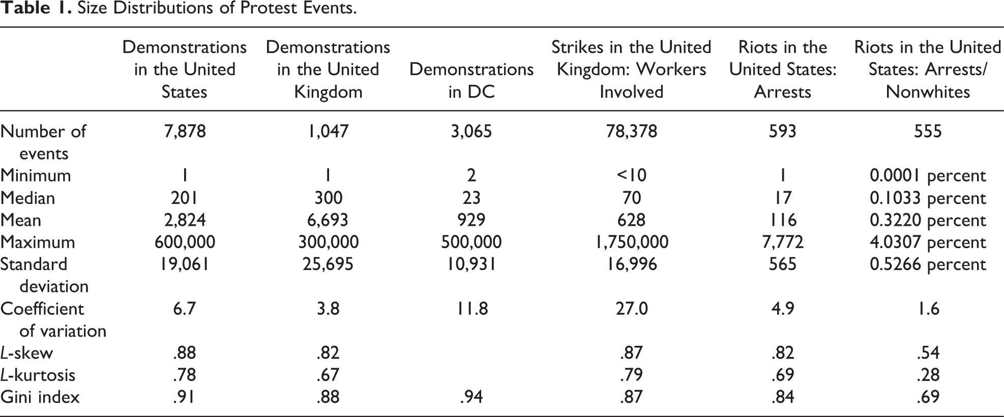
For demonstrations, a single estimate of size is reported in the majority of events in the United States and the United Kingdom (63 percent in DCAUS and 71 percent in EPCD). The remainder are described approximately, as by orders of magnitude. EPCD employs the sensible convention of coding hundreds as 300, thousands as 3,000, and so on.¹⁰ I apply this to DCAUS.¹¹ In both countries, the typical or median size was in the hundreds, while the maximum was in the hundreds of thousands. These distributions underestimate the degree of variation, because the smallest events were much less likely to be reported. It is valuable to compare the exceptionally comprehensive record of demonstrations in Washington, DC (McCarthy et al. 1996:484, 488). Here, the number of participants is usually the number anticipated by organizers when applying for a permit to demonstrate; sometimes it is the number as subsequently amended by the police. The median size was two dozen. The largest demonstration exceeded the median by over four orders of magnitude.

Data on strikes in the United Kingdom cover those lasting for at least a day and involving at least 10 workers, along with small or brief strikes if at least 100 working days were lost. Size is measured by the number of workers involved.¹² Published tabulations use broad size intervals, but fortunately it is possible to identify each individual strike reaching 10,000 workers (see Online Appendix S1). The median was under 100, which is comparable to demonstrations when they are measured comprehensively. The maximum was larger, because a strike does not require the physical assembly of participants in a single place.

For riots, size is proxied by the number of arrests. (Events where no one was arrested are omitted.) The median number of arrests was 17. The maximum—a riot in Washington, DC in April 1968—was greater by over two orders of magnitude. From retrospective surveys in three cities, it is estimated that between one in six and one in three rioters were arrested (Fogelson 1971:36-37). By implication, participation in the largest riots was an order of magnitude smaller than participation in the largest demonstrations. This makes sense given that a major demonstration in a capital city always attracts people from elsewhere, whereas the vast majority of rioters are local. Because a riot is geographically circumscribed, we can also consider the number of arrests in relation to the population of potential rioters, in this case the number of nonwhites in the city.¹³ The median was 0.1 percent. The maximum was greater by an order of magnitude, at 4 percent. Dividing by population significantly reduces variance (as manifested in the coefficient of variation) and kurtosis. Note that the data on riots comprise fewer events than the other data sets. In principle, of course, the maximum will increase with the number of observations, and markedly so for a heavy-tailed distribution. In practice, though, it is hard to conceive of a much greater maximum number of arrests in one city.

All these distributions exhibit enormous variation in size. The standard deviation always exceeded the mean. The least variation occurred in the distribution of riot arrests relative to population; even then the maximum was 40 times the median. The ratio of maximum to median exceeded 20,000 for participants in demonstrations—when not filtered through news media—and in strikes. The typical size is profoundly misleading.

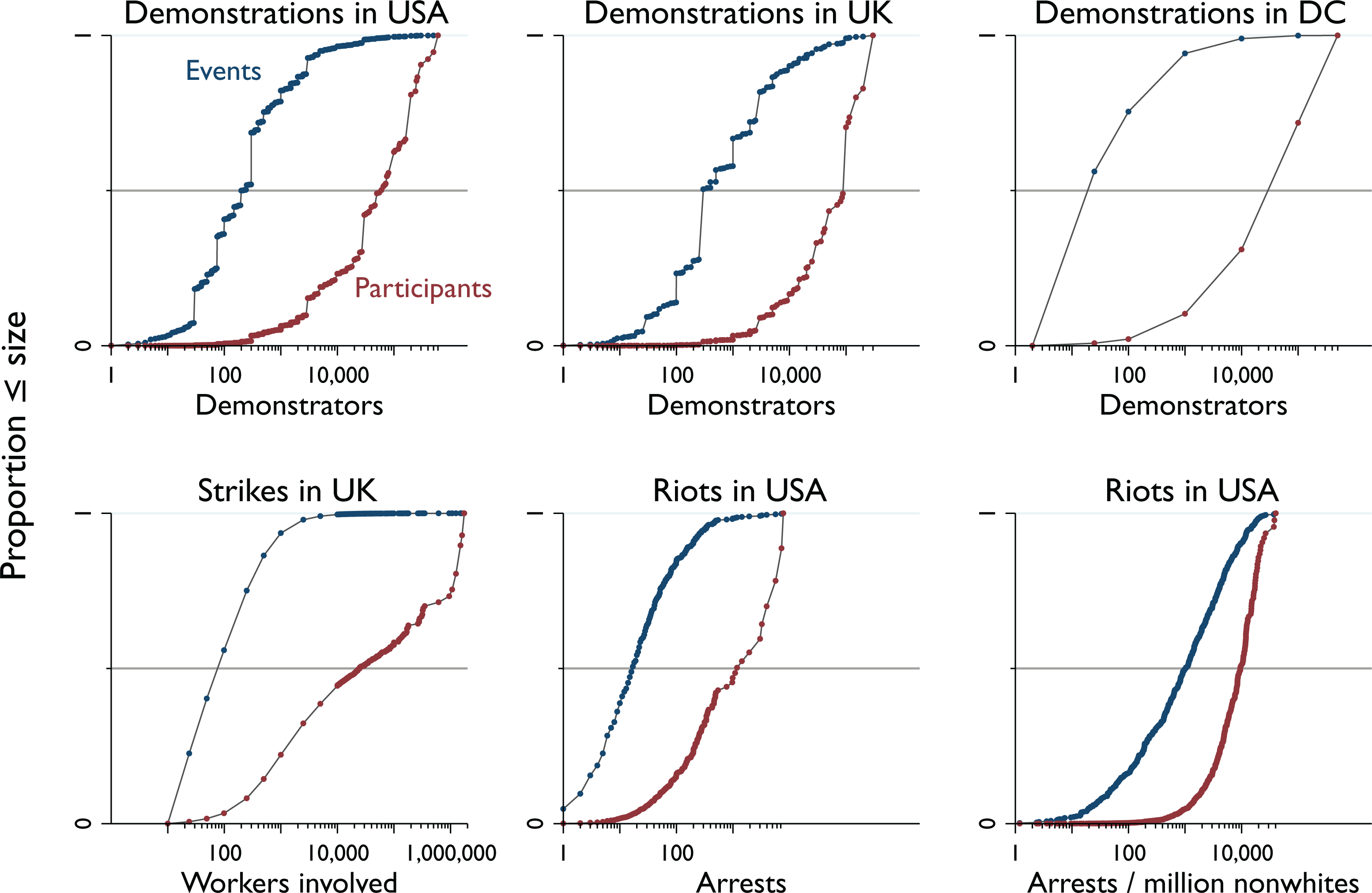
A heavy tail implies “mass-count disparity” (Crovella 2001): Most of the total size comes from a small number of huge events. The literature on protest occasionally notes this feature (Franzosi 1989:352; Koopmans 1995:251; Rucht and Neidhardt 1998:76-77), but its importance has not been fully appreciated. Figure 1 illustrates the disparity by comparing two cumulative distributions (after Feitelson 2006). One is the distribution of events by size. The other, shifted to the right, is the distribution of participants by size of event. The horizontal scale must be logarithmic, of course, to encompass the extreme range. Discontinuities in the graphs for demonstrations in the United States and the United Kingdom are due to size ranges (like thousands) being translated into a number.

Figure 1.

Cumulative size distributions: mass-count disparity.

Comparison of the three graphs for demonstrations reveals the gap left by underreporting. In DC, demonstrations with no more than 25 participants accounted for over half the events. When events were filtered through the news media, the total contained far fewer of these tiny events: 5 percent in the United Kingdom and 7 percent in the United States. Paradoxically, however, the distribution of participation shows that when small events were comprehensively recorded—demonstrations in DC and strikes—they still contributed almost nothing to the total. Total participation was dominated by the largest events, which constituted a tiny fraction of all events. In DC, only 1 percent of demonstrations had more than 10,000 participants, but they accounted for 69 percent of the total demonstrators. For strikes, only 0.4 percent involved as many as 10,000 workers, but they accounted for 56 percent of the total workers involved. In only 1.8 percent of riots did arrests reach 1,000, but they accounted for just over half of the total arrests. For riots, as before, we can adjust for population. One in ten riots led to the arrest of at least 1 percent of the nonwhite population, and these riots accounted for half of the total percentage of nonwhites arrested.

Mass-count disparity is visualized as the gap between the two cumulative distributions. It can be captured in a familiar statistic, the Gini index of inequality, shown in Table 1.¹⁴ For demonstrations, the index ranged from .88 to .94; it was highest for DC because more small events were included.¹⁵ For strikes, the index was .87. These figures indicate extreme inequality. For comparison, the distribution of wealth in the contemporary United States has a Gini index of about .8. The index for arrests was .84. When arrests are denominated by population, the index was .69. The latter is still higher than the index for the distribution of income (before taxes and transfers) in the contemporary United States, about .5.

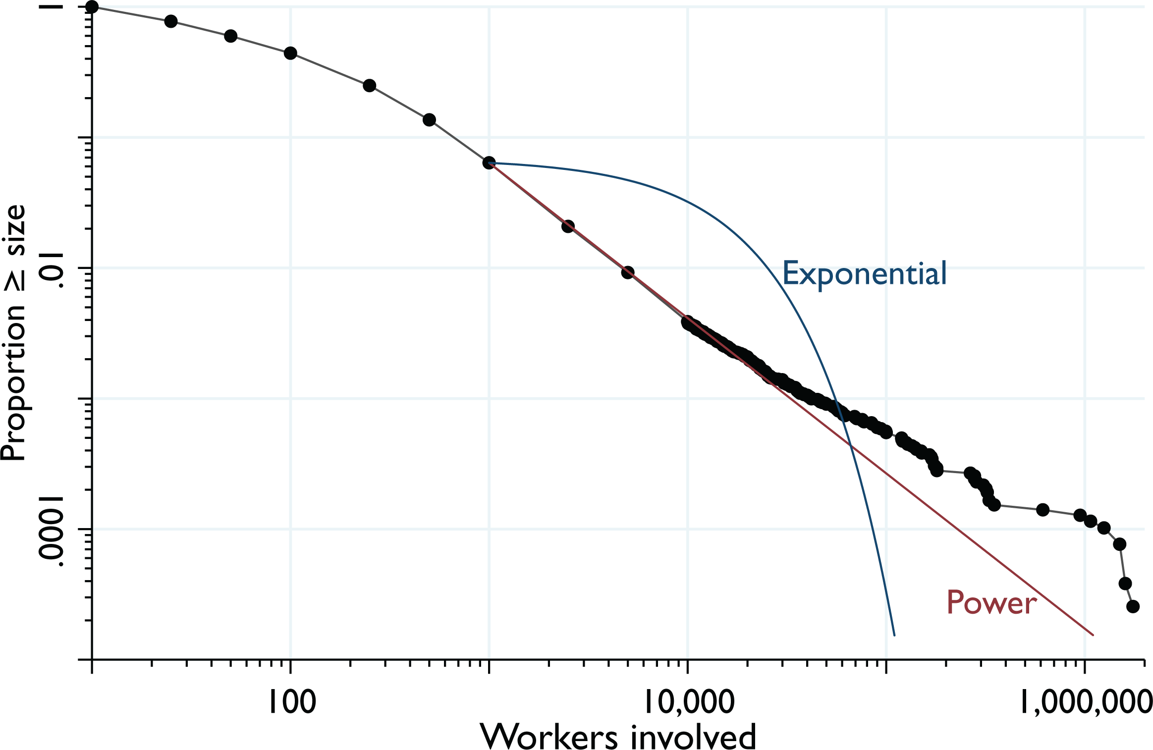
Thus far, I have referred generically to heavy-tailed distributions without considering the shape of the tail. The archetypal heavy tail is the power law, where the probability of an event of size x is proportional to x^−α. In a pioneering study, Richardson (1948) argued that the size of wars, measured by fatalities, followed a power law. The same distribution has been identified in terrorist and insurgent attacks (Bohorquez et al. 2009; Clauset, Young, and Gleditsch 2007). According to Biggs (2005b), strikes in two cities in the late nineteenth century followed a power law, with α estimated as 1.9 to 2.0 (for x ≥ 100–150). Discriminating a power law from other heavy-tailed distributions—such as the lognormal and the power law with exponential cutoff—is empirically demanding. Only a small fraction of events comprises the tail, and so the total number of observations must be very large (Clauset, Shalizi, and Newman 2009). Therefore, it makes sense to concentrate on strikes. Figure 2 plots the complementary cumulative distribution, with both axes on a logarithmic scale. (Online Figure S1 depicts the other data sets.) Following the method of Virkar and Clauset (2014), the power law with the best fit has α of 2.2, starting at 1,000 to 2,499 workers. It appears on the graph as a straight diagonal line. Clearly, this power law does not describe the very upper tail of the distribution; it predicts too few huge strikes. But alternative heavy-tailed distributions (fit to the same tail, starting at 1,000 to 2,499) are inferior.¹⁶ The graph also serves to illustrate the significance of a heavy tail. Recall that heavy means heavier than the exponential distribution. The graph shows the best-fitting exponential distribution, which resembles an inverted J. Such a distribution would predict many more medium-sized strikes and fewer large ones; a strike involving more than a hundred thousand workers would be vanishingly rare. A heavy tail, by contrast, reflects the fact that huge events—more than four orders of magnitude greater than the median, in this case—can occur.

Figure 2.

Strikes in the United Kingdom: complementary cumulative size distribution.

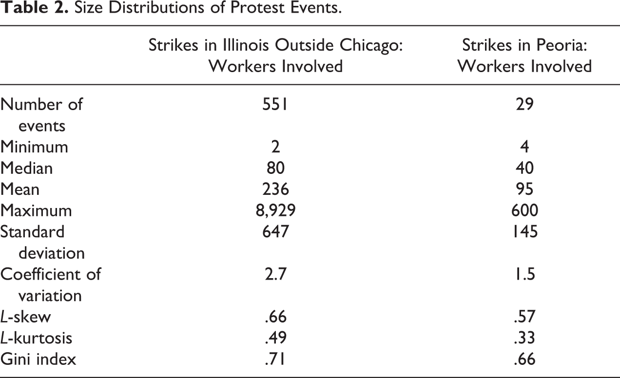
Such huge events occur in data sets that cover a population of many millions over decades; these data sets are the staple of sociological analysis. Does the size distribution differ for small populations? Answering this question requires comprehensive data on small events in minor places, which rules out the media as a source. The best candidate is strikes in the United States between 1881 and 1893 (see Online Appendix S2). At that time, almost all employers were confined to a single location, with the major exception of railroads. Table 2 shows the size distribution for strikes in Illinois outside the industrial metropolis of Chicago (Cook County, to be precise). A few large railroad strikes are omitted because the Commissioner did not specify all their locations; the period ends before the massive Pullman railroad strike in 1894. The size distribution exhibits much less variation than the large national data sets. The coefficient of variation is 2.7, compared to 27 for strikes in the United Kingdom. Mass-count disparity is still significant: Only 5 percent of strikes involved at least 1,000 workers, but these accounted for almost half (44 percent) the total number of participants. Although the largest strike fell short of 10,000 workers, note that the number of events is relatively small. Sampling the same number of events from strikes in the United Kingdom, we would expect only two (0.4 percent) to reach 10,000. Focusing on a particular location further reduces variation in the size of events. Table 2 shows strikes in Peoria, the state’s second city, which had a working-class population of about 8,000. The largest strike involved 600 workers. With so few events, the upper tail of the distribution cannot be estimated; a much larger strike could have been possible. Even so, the Gini index shows greater inequality than is found in the distribution of income.

Table 2.

Size Distributions of Protest Events.

	Strikes in Illinois Outside Chicago: Workers Involved	Strikes in Peoria: Workers Involved
Number of events	551	29
Minimum	2	4
Median	80	40
Mean	236	95
Maximum	8,929	600
Standard deviation	647	145
Coefficient of variation	2.7	1.5
L-skew	.66	.57
L-kurtosis	.49	.33
Gini index	.71	.66

Event Frequency and Total Participation

Sociologists usually choose to count the frequency of events in each time interval or geographical unit. An alternative is to sum the number of participants to yield total participation per interval or unit. This takes into account the enormous variation in the size of events like demonstrations and strikes. It also avoids a problem that has escaped attention in the literature.¹⁷ How is one event to be demarcated from another? In principle, this should be straightforward when dealing with a contentious gathering that is characterized by continuity and contiguity of action, like a march. In practice, however, event catalogs often treat multiple gatherings in different locations as one event. Thus, vigils and processions in 21 cities on “National Free Sharon Kowalski Day” (to support a disabled woman whose lesbian partner was denied access by her family) become a single event in DCAUS. Why not count 21 events? EPCD likewise classifies the annual Loyalist Orange parades throughout Northern Ireland on July 12 as a single event (sometimes entering a particularly large or contentious parade as a second event). Why not consider the parades in each town or city as separate events? These coding decisions apparently reflect the level of detail provided by news reports. The problem of demarcation vanishes if we measure total participation in a time interval. When a newspaper reported “scores of Orange demonstrations in which an estimated 100,000 people took part” (The Times of London, July 13, 1990), whether we treat this as one event or scores makes no difference—either way, total participation increases by 100,000.

Does the choice between total participation and event frequency make a difference in practice? One might expect a high correlation, especially in an annual national time series. After all, there are many protest events in each year: on average, for example, over 200 demonstrations in the United States and over 2,000 strikes in the United Kingdom. When so many events are aggregated, we might suspect that size differences would tend to average out.

Figure 3 traces both time series for demonstrations in the United States. Total participation spikes in 1969 and peaks in 1982. Event frequency peaks in the mid-1960s, declines to the mid-1970s, and then continues at a low level. The two variables follow a completely different trajectory. The scatterplots in Figure 4 portray the association between event frequency and total participation; the linear regression line is dashed. For demonstrations in the United States, the correlation coefficient is only .10. The correlation is somewhat higher for demonstrations in the United Kingdom, albeit for only 16 years. An estimated correlation coefficient automatically increases with fewer observations; in the United States, the correlation for each 16-year subperiod (1960–1975 to 1980–1995) averages .19. For strikes in the United Kingdom, the correlation is low. For strikes in Illinois outside Chicago (not graphed), the correlation is .43, again for a much shorter period. For these time series, the population of potential protesters did not increase sufficiently to require adjustment.¹⁸

Figure 3.

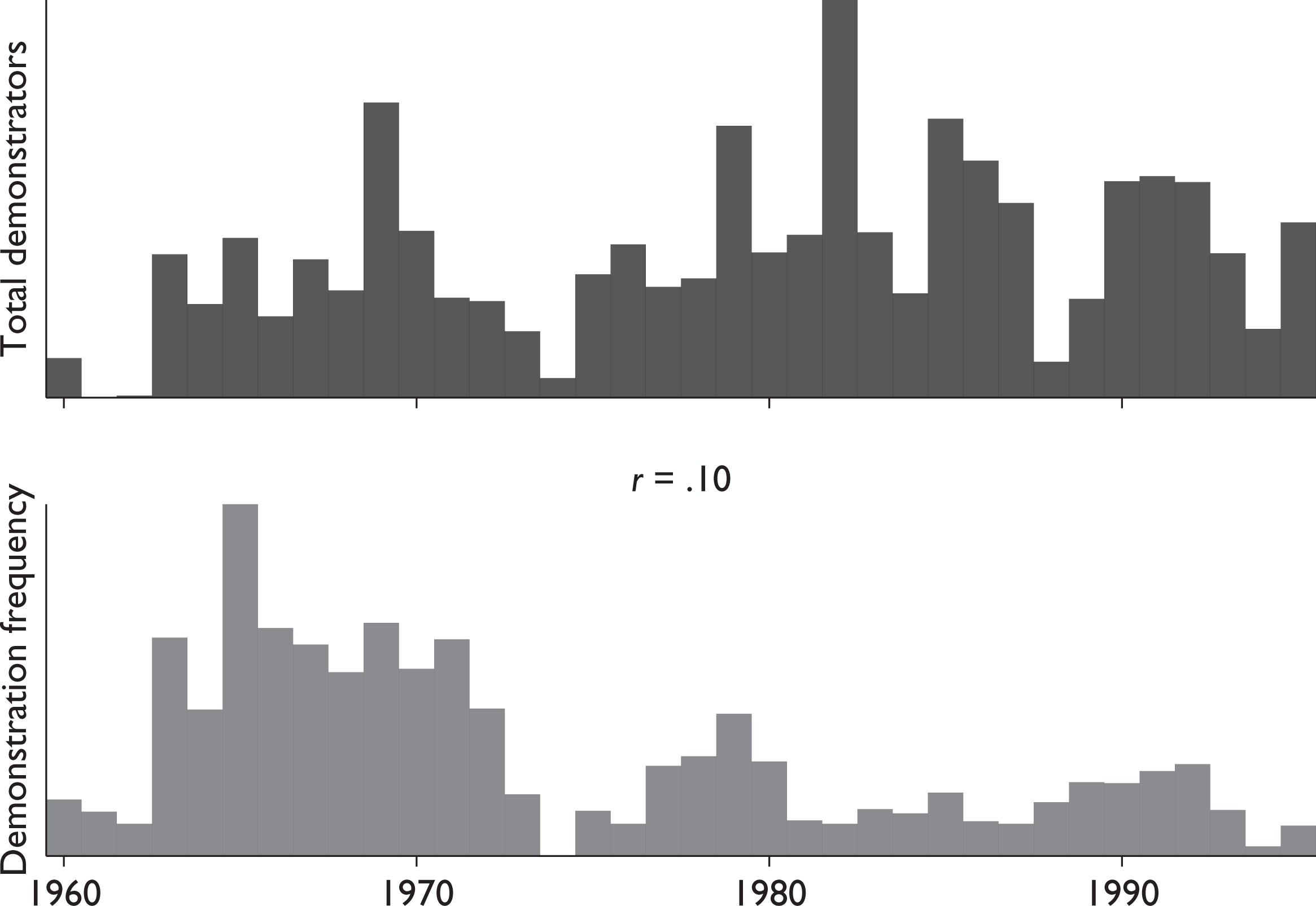
Demonstrations in the United States: total participation and event frequency.

Figure 4.

Event frequency and total participation.

Riots are mapped on to the 460 urban places with a population of at least 25,000 and a nonwhite population of at least 1,000 in 1960. Few events are distributed across many observations, whereas the time series have many events distributed across few observations. The maximum number of riots was 14, in Washington, DC. Half of the cities experienced no riots, and so the regression line (in Figure 4) is anchored at the bottom left-hand corner. The correlation between total arrests and riot frequency is only modest. But it is really necessary to adjust for the tremendous variation in the size of cities. Total participation obviously scales with the population at risk. As argued above, event frequency must scale to population raised to a fractional power; the square root is used here.¹⁹ Thus denominated, riot frequency and total arrests reach the highest correlation, .64. This means that frequency predicts only 41 percent of the variation in per capita arrests.²⁰

In sum, when events like riots and demonstrations are aggregated over time or space, the frequency of events is only minimally or modestly associated with total participation in those events. The divergence between event frequency and total participation partly reflects the heavy-tailed size distribution of events; the occurrence of a huge event significantly increases total participation while only incrementing event frequency. Furthermore, the four annual time series reveal negative correlations between event frequency and average event size; in years with many events, events tended to be smaller. Whether this is coincidental or reflects a more general pattern must await research on other data sets.

These findings do not prove that total participation always diverges from event frequency. For events with minimal variation in size (exemplified by suicide protest), total participation will be practically the same as event frequency. For the staple tactics of social movements, however, there is no justification to assume a high correlation over time or across spatial units. Similar disassociation is evident, for example, for demonstrations in Belarus in the 1990s, aggregated by quarter (Titarenko et al. 2001:137). It follows that the findings from multivariate analysis using event frequency—as either the dependent variable or an independent variable—cannot be assumed to apply to total participation. Likewise, findings using total participation cannot be assumed to apply to event frequency. The choice of measurement is crucial.

The Dominance of Large Events

The fact that protest events vary enormously in size can mitigate a major problem identified in the literature. Most events are not reported by the news media and so are omitted from event catalogs. In Washington, DC, newspapers reported only one in ten demonstrations. Worse, the extent of this underreporting will fluctuate over time—depending, for example, on the significance of other news—in ways that cannot be ascertained. Hence, the argument that newspapers are a seriously flawed source of data (Myers and Caniglia 2004; Ortiz et al. 2005). They are indeed flawed if one wishes to count the frequency of events. But the problem evaporates if one wants to trace total participation over time. After all, the probability of an event being reported increases with the number of participants. Newspapers reported only 3 percent of the demonstrations involving 2 to 25 participants in DC, but they reported 52 percent of the demonstrations with 10,001 to 100,000, and both the demonstrations exceeding 100,000 (McCarthy et al. 1996:488).

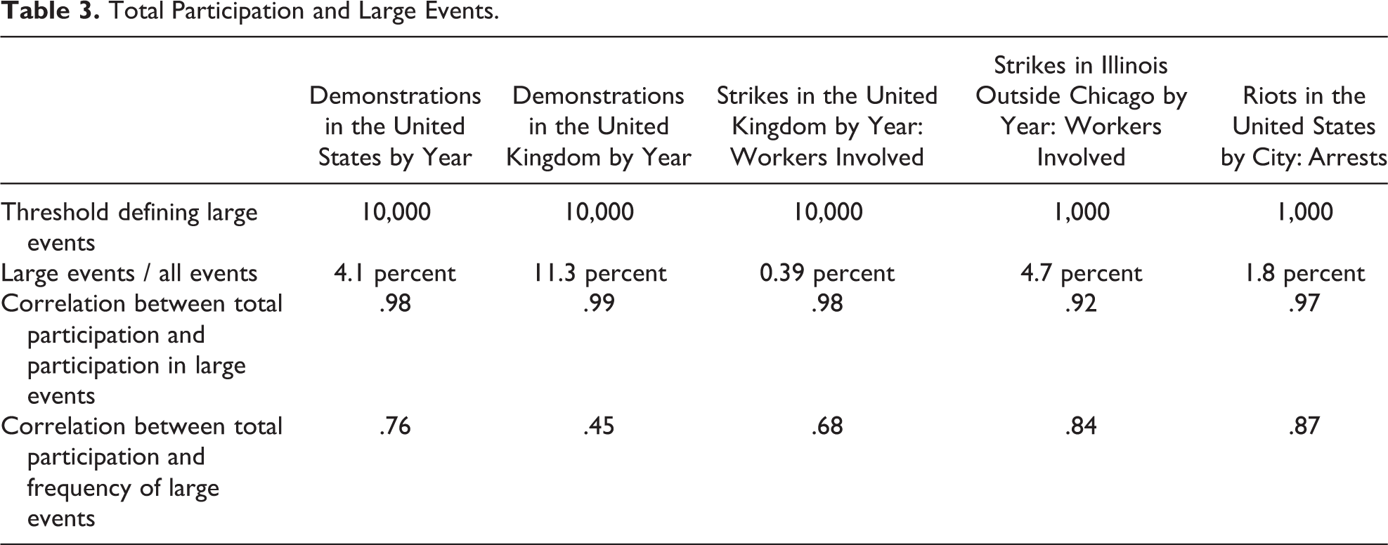
Moreover, mass-count disparity has a surprising implication. When aggregated over time or space, total participation can be predicted by looking only at the large events. What counts as “large” depends on the actual size distribution, of course. We can use the threshold of 10,000 for strikers and demonstrators in the national data sets, and 1,000 for strikers in Illinois and for arrests. Table 3 reports the correlation coefficients. Aggregated by year, the correlations are almost perfect. The result for strikes is especially compelling, because these data do not omit small events. Figure 5 details the total number of workers involved in U.K. strikes reaching various size thresholds. Remarkably, to trace how the total number of strikers fluctuated from year to year, it is possible to ignore 99.6 percent of events; just track the total number of workers involved in strikes of at least 10,000. (This understates the absolute level of participation, of course, but it accurately captures relative change.) Increasing the threshold to the next order of magnitude hardly alters the graph. Even confining attention to strikes involving at least a million workers—only nine events!—captures the salient peaks.

Table 3.

Total Participation and Large Events.

	Demonstrations in the United States by Year	Demonstrations in the United Kingdom by Year	Strikes in the United Kingdom by Year: Workers Involved	Strikes in Illinois Outside Chicago by Year: Workers Involved	Riots in the United States by City: Arrests
Threshold defining large events	10,000	10,000	10,000	1,000	1,000
Large events / all events	4.1 percent	11.3 percent	0.39 percent	4.7 percent	1.8 percent
Correlation between total participation and participation in large events	.98	.99	.98	.92	.97
Correlation between total participation and frequency of large events	.76	.45	.68	.84	.87

Figure 5.

Strikes in the United Kingdom: Workers involved in events of varying size.

Given the dominance of large events, it may be tempting to count their frequency rather than to sum their participants. McAdam and Su (2002), for example, count the frequency of events exceeding 10,000 participants. A heavy tail, however, implies that large events also manifest mass-count disparity; most are moderately large, while a few are massive. Table 3 compares the correlation between total participation and the frequency of large events. The correlation is consistently lower, and it is greatly inferior for U.K. demonstrations.

The problem of underreporting, which has preoccupied the literature on protest events, shrinks when mass-count disparity is understood. For analysis of protest over time at the national level, the problem is readily overcome if we measure total participation rather than event frequency. Total participation is dominated by large events, and large events are most likely to be reported. This reassurance does not hold for the cross-sectional analysis of protesters denominated by population, because a national newspaper may not bother reporting a relatively large event in a small city.

Mass-count disparity does, however, highlight another issue. Because large events are so important, errors affecting them have severe repercussions. Both DCAUS and EPCD erroneously duplicate some demonstrations with hundreds of thousands of participants. One duplicate, for example, increases the year’s total participants by 55 percent! Coding errors are inevitable in assembling a large data set from news reports. Happily, mass-count disparity means that validation can focus on large events, which constitute only a tiny fraction of all events. In DCAUS, for example, only 4 percent of demonstrations reached 10,000 participants. Aside from errors, uncertainty in estimating the size of large events is also a significant concern. When estimates are wildly discrepant—if, for example, the higher is more than double the lower—the decision on which size to use will make a difference. When collecting data, therefore, it will be crucial to record varying estimates and their provenance. Estimates derived from spatial calculation (area occupied and density of demonstrators) are obviously preferable. Even without the benefit of such calculation, one could consistently select estimates with the same direction of bias, for example, using the optimistic figures provided by the organizers.

Conclusion

The study of social movements requires the quantification of protest. What explains protest? What does protest explain? Whether we treat protest as an effect and seek its causes, or treat protest as a cause and seek its effects, we need to differentiate less protest from more. This basic distinction between less and more is required even for explanations that are pursued with qualitative evidence rather than statistical analysis; an historical narrative typically graphs the time series of protest. The pioneers of protest event analysis devoted serious thought to what should be measured and how (e.g., Tilly and Rule 1965). As data accumulated, thanks to their efforts, these crucial issues faded from view.²¹

The choice of how to quantify protest is fundamental, and this has not been fully appreciated. Aggregated over time intervals or across geographical units, there is no high correlation between event frequency and total participation. Four time series yield correlation coefficients from .10 to .43; with city as the unit of observation, the coefficient does not exceed .64. Perhaps other data sets will reveal higher correlations, but this will need to be demonstrated. As it stands, the frequency of events and the total number of participants diverge so much that findings for one are unlikely to apply to the other.

Event frequency has become the default variable in studies of protest. There are numerous points in its favor. It does not require the measurement of the size of events, which is always subject to uncertainty (and may even be impossible when using fragmentary historical records). It enables the aggregation of diverse phenomena, from hunger strikes to press conferences, into a single metric. Using the most commonly used variable has the advantage of facilitating comparison with previous work. Nevertheless, event frequency requires the assumption that size does not matter. To put this tangibly, it assumes that two events represent twice as much as protest as one event, even if the two events are each attended by only 10 participants whereas the single event attracts a million people. The findings of most quantitative work on protest rest on this assumption. Whether this assumption is justified depends ultimately on theory. Event frequency is obviously appropriate for testing theories that explain variation in the number of events, and theories in which the effect of protest depends on the number of events, irrespective of size. When events are counted from news media, underreporting will continue to pose a fundamental methodological challenge. Event frequency, as measured, represents a small proportion of all events, and this proportion fluctuates over time and across space. Two other challenges must also be solved. One is to explicate consistent criteria to demarcate one event from another. Another is to choose an appropriate fractional power when adjusting for population size.

Total participation has several countervailing advantages. Measuring the number of actions—thus, when divided by population, the individual’s hazard of participating—follows naturally from the conception of protest as collective action. Theories often postulate that the effect of protest increases with the total number of participants. In practice, movements act as if they are trying to mobilize more people. Alongside these theoretical considerations, empirical findings highlight the significance of size. Measured by participants, the size distribution of events—like demonstrations, strikes, and riots—does not range modestly around a typical value. Such protest events have a heavy tail: most events are small, but a few are massive. Even when we confine attention to events in one small city (like strikes in Peoria) or divide participants by population (as with riots), there is pronounced inequality in size. How far does this generalization hold? It does not apply to every form of protest; an exception is suicide protest. It may not apply in some social contexts.²² But the generalization does hold for the protest events that are the staple of sociological analysis.²³

Extreme variation in size has positive implications for measurement. With a heavy-tailed distribution, the weight of the distribution is concentrated at the top. Most protesters participate in large events. The underreporting of small events matters less for participation than for event frequency, because small events contribute only a small fraction of the total number of participants. The national series of demonstrations and strikes analyzed here are dominated by events involving at least 10,000 participants. It is important to emphasize that large is relative rather than absolute, and so it varies with the population of potential protesters. In Peoria in the 1880s, for example, a large strike was one that involved hundreds of workers. When aggregated over time or space, the total number of participants is very highly correlated with the total number in the largest events. By implication, attention should focus on the accurate recording of these events. One issue is the estimation of size. Varying estimates of the same event establish lower and upper bounds, which can be used to check the sensitivity of empirical findings. For contemporary events, the huge volume of photographic and video evidence can surely be exploited to refine estimates of crowd size.²⁴ Another issue is the validation of data. The duplication of large events in data sets—identified here in both DCAUS and EPCD—can severely distort empirical results. Fortunately, of course, there are only a small number of large events, and so it is feasible to check them thoroughly.

My argument has two further implications for future research. I have focused on one measure of size: the number of participants. Arguably, this variable is most appropriate when explaining the origins of protest, as it measures the number of individual decisions to participate. When using protest as an explanation for subsequent outcomes, however, participant-days—incorporating the second dimension, duration—could be preferable. There are alternative measures of size, such as severity (e.g., Carter 1986), which also deserve further examination. The point of my argument is not to impose one single variable for all theoretical purposes but to encourage the investigation of size.

The size distribution of protest events has implications beyond method. A significant task for theory is to explain why most protest events are small while a few are huge. One simple explanation is that this distribution reflects the division between populations of potential protesters. The population of cities, for example, follows a power law with α of 2 (Rozenfeld et al. 2011). Thus, the distribution of riot arrests is partly a function of the distribution of population; the heavy tail is significantly diminished when arrests are expressed per capita. Evaluating this explanation for other types of protest is more complicated, because it is hard to conceive of preexisting population divisions for strikes—though the distribution of workers by industry or occupation could be considered—or for demonstrations. A second explanation is that the size distribution reveals something about the process generating protest events. Biggs (2005b) argues for positive feedback: for an event in progress, the larger it becomes, the more likely people are to join it. This kind of process—synonymous with cumulative advantage or preferential attachment—is often used to explain heavy-tailed size distributions (e.g., Seguin 2016). Other models of the generative process are also possible. For violent attacks, a model of the fusion and fission of insurgent groups predicts the distribution of fatalities (Clauset and Weigel 2010; Johnson et al. 2006). Modeling the size of protest events is a promising avenue for future research.

Supplemental Material

Supplemental Material, Supplement_SMR629166 - Size Matters: Quantifying Protest by Counting Participants

Supplemental Material, Supplement_SMR629166 for Size Matters: Quantifying Protest by Counting Participants by Michael Biggs in Sociological Methods & Research

Supplemental Material

Supplemental Material, Supplement_SMR629166 - Size Matters: Quantifying Protest by Counting Participants

Supplemental Material, Supplement_SMR629166 for Size Matters: Quantifying Protest by Counting Participants by Michael Biggs in Sociological Methods & Research

Footnotes

Author’s Note

This article is possible because other scholars have generously shared their data: Gregg Carter; Ronald Francisco; Doug McAdam, John McCarthy, Susan Olzak, and Sarah Soule; Helen Margetts and Scott Hale. It uses software written by Nicholas J. Cox, Zurab Sajaia, and Yogesh Virkar. Kenneth T. Andrews and Charles Seguin subjected a draft to judicious critique, while Tak Wing Chan and Neil Ketchley supplied refreshment and encouragement. Andrew Gelman’s blog convinced me that measurement is worth taking seriously. The unexpurgated version is available as Oxford Sociology Working Paper No. 2015-05 ().

Declaration of Conflicting Interests

The author(s) declared no potential conflicts of interest with respect to the research, authorship, and/or publication of this article.

Funding

The author(s) received no financial support for the research, authorship, and/or publication of this article.

Notes

Supplemental Material

Supplementary material for this article is available online.

References

Amenta

Edwin

Caren

Neal

Chiarello

Elizabeth

Yang

. 2010. “The Political Consequences of Social Movements.” Annual Review of Sociology 36:287–307.

Barranco

José

Wisler

Dominique

. 1999. “Validity and Systematicity of Newspaper Data in Event Analysis.” European Sociological Review 15:301–22.

Biggs

Michael

. 2005a. “Dying without Killing: Self-immolations, 1963-2002.” Pp. 173–208 in Making Sense of Suicide Missions, edited by Gambetta

Diego

. Oxford, UK: Oxford University Press.

Biggs

Michael

. 2005b. “Strikes as Forest Fires: Chicago and Paris in the Late 19th Century.” American Journal of Sociology 110:1684–14.

Biggs

Michael

. 2013. “How Repertoires Evolve: The Diffusion of Suicide Protest in the Twentieth Century.” Mobilization 18:407–28.

Biggs

Michael

. 2015. “Has Protest Increased since the 1970s? How a Survey Question Can Construct a Spurious Trend.” British Journal of Sociology 66:141–62.

Bohorquez

Juan Camilo

Gourley

Sean

Dixon

Alexander R.

Spagat

Michael

Johnson

Neil F.

. 2009. “Common Ecology Quantifies Human Insurgency.” Nature 461:911–14.

Budros

Art

. 2011. “Explaining the First Emancipation: Social Movements and Abolition in the U.S. North, 1776-1804.” Mobilization 16:439–54.

Carter

Gregg Lee

. 1986. “The 1960s Black Riots Revisited: City Level Explanations of Their Severity.” Sociological Inquiry 56:210–28.

10.

Checchi

Daniele

Visser

Jelle

. 2005. “Pattern Persistence in European Trade Union Density: A Longitudinal Analysis 1950-1996.” European Sociological Review 21:1–21.

11.

Choi-Fitzpatrick

Austin

Juskauskas

Tautvydas

. 2015. “Up in the Air: Applying the Jacobs Crowd Formula to Drone Imagery.” Procedia Engineering 107:273–81.

12.

Clauset

Aaron

Shalizi

Cosma Rohilla

Newman

M. E. J.

. 2009. “Power-law Distributions in Empirical Data.” SIAM Review 51:661–703.

13.

Clauset

Aaron

Wiegel

Frederik W.

. 2010. “A Generalized Aggregation-Disintegration Model for the Frequency of Severe Terrorist Attacks.” Journal of Conflict Resolution 54:179–97.

14.

Clauset

Aaron

Young

Maxwell

Gleditsch

Kristian Skrede

. 2007. “On the Frequency of Severe Terrorist Events.” Journal of Conflict Resolution 51:1–31.

15.

Crovella

Mark E.

2001. “Performance Evaluation with Heavy Tailed Distributions.” Pp. 1–10 in Job Scheduling Strategies for Parallel Processing: 7th International Workshop, edited by Feitelson

Dror G.

Rudolph

Larry

. Berlin, Germany: Springer Verlag.

16.

DeNardo

James

. 1985. Power in Numbers: The Political Strategy of Protest and Rebellion. Princeton, NJ: Princeton University Press.

17.

Earl

Jennifer

Martin

Andrew

McCarthy

John D.

Soule

Sarah A.

. 2004. “The Use of Newspaper Data in the Study of Collective Action.” Annual Review of Sociology 30:65–80.

18.

Feitelson

Dror G.

2006. “Metrics for Mass-count Disparity.” Pp. 61–68 in Proceedings of the 14th IEEE International Symposium on Modeling, Analysis, and Simulation of Computer and Telecommunication Systems (MASCOTS ’06). Washington, DC: IEEE Computer Society.

19.

Fogelson

Robert M.

1971. Violence as Protest: A Study of Riots and Ghettos. New York: Doubleday.

20.

Francisco

Ronald A.

n.d. European Protest and Coercion Data, 1980–1995 (computer file). Retrieved December 18, 2012 (http://web.ku.edu/∼ronfrand/data/index.html).

21.

Franzosi

Roberto

. 1987. “The Press as a Source of Socio-historical Data: Issues in the Methodology of Data Collection from Newspapers.” Historical Methods 20:5–15.

22.

Franzosi

Roberto

. 1989. “One Hundred Years of Strike Statistics: Methodological and Theoretical Issues in Quantitative Strike Research.” Industrial and Labor Relations Review 42:348–62.

23.

Haines

Michael R.

and Inter-university Consortium for Political and Social Research. 2010. Historical, Demographic, Economic, and Social Data: The United States, 1790–2002. ICPSR 02896-v3 (computer file). Ann Arbor, MI: Inter-university Consortium for Political and Social Research.

24.

Hibbs

Douglas A.

1973. Mass Political Violence: A Cross-National Causal Analysis. New York: John Wiley and Sons.

25.

Hosking

J. R. M.

1990. “L-moments: Analysis and Estimation of Distributions Using Linear Combinations of Order Statistics.” Journal of the Royal Statistical Society, Series B 52:105–24.

26.

Inclán

María

. 2009. “Sliding Doors of Opportunity: Zapatistas and Their Cycle of Protest.” Mobilization 14:85–106.

27.

Jacobs

David

Kent

Stephanie L.

. 2007. “The Determinants of Executions since 1951: How Politics, Protests, Public Opinion, and Social Divisions Shape Capital Punishment.” Social Problems 54:297–318.

28.

Jenkins

J. Craig

Jacobs

David

Agnone

Jon

. 2003. “Political Opportunities and African-American Protest, 1948–1997.” American Journal of Sociology 109:277–303.

29.

Johnson

Neil F.

Spagat

Mike

Restrepo

Jorge A.

Becerra

Oscar

Bohorquez

Juan Camilo

Suarez

Nicolas

Restrepo

Elvira Maria

Zarama

Roberto

. 2006. “Universal Patterns Underlying Ongoing Wars and Terrorism.” Retrieved October 27, 2010 (http://xxx.lanl.gov/abs/physics/0605035).

30.

Koopmans

Ruud

. 1995. Democracy from Below: New Social Movements and the Political System in West Germany. Boulder, CO: Westview.

31.

Kriesi

Hanspeter

Koopmans

Ruud

Dyvendak

Jan Willem

Giugni

Marco G.

. 1995. New Social Movements in Western Europe: A Comparative Analysis. Minneapolis: University of Minnesota Press.

32.

Lohmann

Susanne

. 1994. “The Dynamics of Informational Cascades: The Monday Demonstrations in Leipzig, East Germany, 1989–91.” World Politics 47:42–101.

33.

Maney

Gregory M.

Oliver

Pamela E.

. 2001. “Finding Collective Events: Sources, Searches, Timing.” Sociological Methods and Research 30:131–69.

34.

Mann

Leon

. 1974. “Counting the Crowd: Effects of Editorial Policy on Estimates.” Journalism Quarterly 51:278–85.

35.

Margetts

Helen

John

Peter

Hale

Scott

Yasseri

Taha

. 2016. Political Turbulence: How Social Media Shape Collective Action. Princeton, NJ: Princeton University Press.

36.

McAdam

Doug

. 1982. Political Process and the Development of Black Insurgency. Chicago: University of Chicago Press.

37.

McAdam

Doug

McCarthy

John D.

Olzak

Susan

Soule

Sarah A.

. n.d. Dynamics of Collective Action in the United States (computer file). Retrieved July 1, 2012 (http:www.stanford.edu/group/collectiveaction/).

38.

McAdam

Doug

Yang

. 2002. “The War at Home: Antiwar Protests and Congressional Voting, 1965 to 1973.” American Sociological Review 67:696–721.

39.

McCarthy

John D.

McPhail

Clark

Smith

Jackie

. 1996. “Images of Protest: Dimensions of Selection Bias in Media Coverage of Washington Demonstrations, 1982 and 1991.” American Sociological Review 61:478–99.

40.

McCarthy

John D.

McPhail

Clark

Smith

Jackie

Crishock

Louis J.

. 1998. “Electronic and Print Media Representations of Washington D.C. Demonstrations, 1982 and 1991: A Demography of Description Bias.” Pp. 113–30 in Acts of Dissent: New Developments in the Study of Protest, edited by Rucht

Dieter

Koopmans

Ruud

Neidhardt

Friedhelm

. Berlin, Germany: Edition Sigma.

41.

McCarthy

John D.

Titarenko

Larissa

McPhail

Clark

Rafail

Patrick S.

Augustyn

Boguslaw

. 2008. “Assessing Stability in the Patterns of Selection Bias in Newspaper Coverage of Protest during the Transition from Communism in Belarus.” Mobilization 13:127–46.

42.

McPhail

Clark

McCarthy

John

. 2004. “Who Counts and How: Estimating the Size of Protests.” Contexts 3:12–18.

43.

Morgan

William R.

Clark

Terry Nichols

. 1973. “The Causes of Racial Disorders: A Grievance-level Explanation.” American Sociological Review 38:611–24.

44.

Myers

Daniel J.

2010. “Violent Protest and Heterogeneous Diffusion Processes: The Spread of U.S. Racial Rioting from 1964 to 1971.” Mobilization 15:289–321.

45.

Myers

Daniel J.

Caniglia

Beth Schaefer

. 2004. “All the Rioting That’s Fit to Print: Selection Effects in National Newspaper Coverage of Civil Disorders, 1968–1969.” American Sociological Review 69:519–43.

46.

Oberschall

Anthony R.

1994. “Rational Choice in Collective Protests.” Rationality and Society 6:79–100.

47.

Oliver

Pamela E.

Maney

Gregory

. 2000. “Political Processes and Local Newspaper Coverage of Protest Events: From Selection Bias to Triadic Interactions.” American Journal of Sociology 106:463–505.

48.

Oliver

Pamela E.

Myers

Daniel J.

. 1999. “How Events Enter the Public Sphere: Conflict, Location, and Sponsorship in Local Newspaper Coverage of Public Events.” American Journal of Sociology 105:38–87.

49.

Oliver

Pamela E.

Myers

Daniel J.

. 2003. “The Coevolution of Social Movements.” Mobilization 8:1–24.

50.

Olzak

Susan

. 1989. “Analysis of Events in the Study of Collective Action.” Annual Review of Sociology 15:119–41.

51.

Olzak

Susan

. 1992. The Dynamics of Ethnic Competition and Conflict. Stanford, CA: Stanford University Press.

52.

Opp

Karl-Dieter

. 2009. Theories of Political Protest and Social Movements: A Multidisciplinary Introduction, Critique, and Synthesis. Abingdon, UK: Routledge.

53.

Ortiz

David G.

Myers

Daniel J.

Walls

Eugene N.

Diaz

Maria-Elena D.

. 2005. “Where Do We Stand with Newspaper Data?” Mobilization 10:397–419.

54.

Popovic

Srdja

Miller

Matthew

. 2015. Blueprint for Revolution: How to Use Rice Pudding, Lego Men, and Other Non-violent Techniques to Galvanise Communities, Overthrow Dictators, or Simply Change the World. Melbourne, Australia: Scribe.

55.

Przeworski

Adam

. 2009. “Conquered or Granted? A History of Suffrage Extensions.” British Journal of Political Science 39:291–321.

56.

Resnick

Sidney I.

2010. Heavy-tail Phenomena: Probabilistic and Statistical Modeling. New York: Springer.

57.

Richardson

Lewis F.

1948. “Variation of the Frequency of Fatal Quarrels with Magnitude.” Journal of the American Statistical Association 43:523–46.

58.

Rosenfeld

Jake

. 2006. “Desperate Measures: Strikes and Wages in Post-Accord America.” Social Forces 85:235–65.

59.

Rozenfeld

Hernán D.

Rybski

Diego

Gabaix

Xavier

Makse

Hernán A.

. 2011. “The Area and Population of Cities: New Insights from a Different Perspective on Cities.” American Economic Review 101:2205–25.

60.

Rucht

Dieter

Neidhardt

Friedhelm

. 1998. “Methodological Issues in Collecting Protest Event Data: Units of Analysis, Sources and Sampling, Coding Problems.” Pp. 65–89 in Acts of Dissent: New Developments in the Study of Protest, edited by Rucht

Dieter

Koopmans

Ruud

Neidhardt

Friedhelm

. Berlin, Germany: Edition Sigma.

61.

Rummel

Rudolph J.

1963. “Dimensions of Conflict Behavior within and between Nations.” General Systems Yearbook 8:1–50.

62.

Seguin

Charles

. 2016. “Cascades of Coverage: Dynamics of Media Attention to Social Movement Organizations.” Social Forces 94:997–1020.

63.

Shorter

Edward

Tilly

Charles

. 1974. Strikes in France, 1830-1968. New York: Cambridge University Press.

64.

Soule

Sarah A.

Earl

Jennifer

. 2005. “A Movement Society Evaluated: Collective Protest in the United States.” Mobilization 10:345–64.

65.

Spielmans

John V.

1944. “Strike Profiles.” Journal of Political Economy 52:319–39.

66.

Tarrow

Sidney

. 1989. Democracy and Disorder: Protest and Politics in Italy, 1965–1975. Oxford, UK: Clarendon Press.

67.

Tarrow

Sydney

. 2011. Power in Movement: Social Movements, Collective Action, and Politics. 3rd ed. New York: Cambridge University Press.

68.

Tilly

Charles

. 1978. From Mobilization to Revolution. New York: McGraw-Hill.

69.

Tilly

Charles

. 1995. Popular Contention in Great Britain, 1758–1834. Cambridge, MA: Harvard University Press.

70.

Tilly

Charles

Rule

James B.

. 1965. Measuring Political Upheaval. Princeton, NJ: Centre of International Studies, Princeton University.

71.

Titarenko

Larissa

McCarthy

John D.

McPhail

Clark

Augustyn

Boguslaw

. 2001. “The Interaction of State Repression, Protest Form and Protest Sponsor Strength during the Transition from Communism in Minsk, Belarus, 1990–1995.” Mobilization 6:129–50.

72.

U.S. Bureau of the Census. 1960. Census of Population, 1960, Vol. 1, Characteristics of the Population, parts 2-52. Washington, DC: Government Printing Office.

73.

Virkar

Yogesh

Clauset

Aaron

. 2014. “Power-law Distributions in Binned Empirical Data.” Annals of Applied Statistics 8:89–119.

74.

Yip

Paul S. F.

Watson

Ray

Chan

K. S.

Lau

Eric H. Y.

Chen

Feng

Ying

Liqun

Cheung

Derek Y. T.

Brian Y. T.

Liu

Danping

. 2010. “Estimation of the Number of People in a Demonstration.” Australian and New Zealand Journal of Statistics 52:17–26.

Supplementary Material

Please find the following supplemental material available below.

For Open Access articles published under a Creative Commons License, all supplemental material carries the same license as the article it is associated with.

For non-Open Access articles published, all supplemental material carries a non-exclusive license, and permission requests for re-use of supplemental material or any part of supplemental material shall be sent directly to the copyright owner as specified in the copyright notice associated with the article.

0.02 MB

0.00 MB

0.29 MB