The Case for Selecting Cases That Are Deviant or Extreme on the Independent Variable

Abstract

Qualitative and multimethod scholars face a wide and often confusing array of alternatives for case selection using the results of a prior regression analysis. Methodologists have recommended alternatives including selection of typical cases, deviant cases, extreme cases on the independent variable, extreme cases on the dependent variable, influential cases, most similar cases, most different cases, pathway cases, and randomly sampled cases, among others. Yet this literature leaves it substantially unclear which of these approaches is best for any particular goal. Via statistical modeling and simulation, I argue that the rarely considered approach of selecting cases with extreme values on the main independent variable, as well as the more commonly discussed deviant case design, are the best alternatives for a broad range of discovery-related goals. By contrast, the widely discussed and advocated typical case, extreme-on-Y, and most similar cases approaches to case selection are much less valuable than scholars in the qualitative and multimethods research traditions have recognized to date.

Keywords

case selection multimethod case study qualitative regression

Introduction

In the context of ongoing scholarly interest in multimethod analysis in the social sciences (e.g., Dunning 2012; Glynn and Ichino 2015; Lieberman 2005; Poteete, Janssen, and Ostrom 2010; Small 2011), case study scholars are facing increasing pressures to coordinate their research with (their own or prior) regression-type quantitative analysis. Obviously, not all important case study research—historically or in the future—is in close dialogue with existing quantitative research. Some case studies break new substantive ground, such that there is little or no relevant statistical data or analysis with which they could interact. Yet in most of the major debates on big questions in the social sciences, there are influential studies in both the quantitative and the qualitative traditions.

Hence, there are usually intellectual gains to be made from case studies that push forward an existing regression analysis, and many scholars have in practice implemented designs in which cases are selected for in-depth analysis after a regression or related statistical analysis. For example, Huber and Stephens (2012) use a cross-national statistical analysis of the determinants of social policy spending in Latin America as a framework for selecting case studies (pp. 47-52), Ziblatt (2009) selects case studies from a time-series cross-sectional analysis of electoral fraud claims in German constituencies (p. 14), and Baccini and Urpelainen (2014) justify a case study investigation of trade and liberalization politics in South Africa based on that country’s low residual in a regression analysis (p. 201).

Before a scholar can begin this kind of case study research to test, refine, or interpret a regression analysis, a surprisingly complex prior challenge needs to be addressed: selecting cases for in-depth analysis from the comparatively large data set necessary for regression. Seawright and Gerring (2008) have proposed a set of systematic case selection rules as a solution to this challenge. Yet the question remains, which of the several available methods should be used in a given project? Several scholars arguing in favor of deliberate case selection have focused on three of these alternatives: typical cases, deviant cases, and extreme cases on the dependent variable.¹ Others have argued for random sampling (Fearon and Laitin 2008:764-66) or deliberate sampling intended to represent the full range of variation in the data (King, Keohane, and Verba 1994:139-46).

I argue that the existing advice is incomplete or misleading when the goal of case study research is discovery. I develop this argument by showing that, across a wide range of goals, the alternatives with the best chances of facilitating discovery are either deviant case selection or the rarely discussed alternative of selecting extreme cases on the main independent variable.² This argument is developed with reference to a variety of discovery-related goals: searching for sources of measurement error in the dependent or key independent variables; testing for or trying to discover an omitted variable, which may or may not be correlated with the independent variable of interest; exploring hypotheses about causal pathways; finding a case with a causal effect close to the population mean; and discovering substantive sources of causal heterogeneity.

Unlike much existing research on qualitative and case study methods, this discussion is not driven by reference to examples of excellent research. In many other kinds of qualitative research practices, the analyst’s judgment is a central ingredient in the application of the research tool; as a consequence, there is a great deal to learn from studying how judgment was employed in notably successful applications of the research tools in question. By contrast, systematic case selection is an algorithmic process: It takes a certain kind of information as an input and then follows logical or mathematical rules to convert that input into a case. Because systematic case selection rules reduce scholars’ reliance on judgment, the statistical properties of case selection algorithms are more important than notably successful examples of their application. For this reason, the discussion below asks qualitative scholars and methodologists to follow statistical reasoning about case selection in the absence of famous examples.

In practice, of course, scholars will not always rely solely on systematic case selection to design qualitative research, since considerations of data availability, the substantive prominence of cases, and other practical concerns must sometimes be balanced with selection of the case most likely to meet a given goal. Future research analyzing the balance between such considerations in practice and offering guidance to scholars for how to handle such competing priorities would be useful.

Case Selection Techniques: A Brief Overview

In making the argument that discovery is best facilitated through the selection of deviant or extreme-on-X cases, it is important to consider a broad and inclusive set of alternative case selection rules. Inclusiveness, after all, forestalls the possible objection that the best alternatives were simply not considered. For this purpose, it is helpful that Seawright and Gerring (2008) provide a broad menu of formal rules for case selection in the wake of a regression analysis, combining ideas from qualitative methodology in the social sciences and from the statistical literature on regression diagnostics. Here, I will briefly introduce those techniques and provide the formulas or other steps necessary for implementation before continuing to the analysis of each decision rule’s statistical properties with respect to the diverse set of research goals considered here. This section will also present a case selection technique developed by Plumper, Troeger, and Neumayer (2010), which is effectively a hybrid of extreme and most similar case selection rules, as well as an algorithm discussed by Gerring (2007a) that turns out to be closely related to existing techniques. This will provide an inclusive, although not necessarily comprehensive, comparison set against which to demonstrate the virtues of selecting deviant and extreme-on-X cases. Before introducing these techniques, however, it is useful to discuss a set of research goals for which they might be used.

Major Goals of Case Study Research

Researchers obviously have many goals for case study analysis. It is impossible to give a comprehensive account of such goals, and some desirable goals such as elucidating causally relevant counterfactuals via case study research (Glynn and Ichino 2015) are difficult to systematize, given their early state of development in the literature on qualitative methods. For present purposes, it will suffice to consider a broad collection of common goals—some widely applicable in qualitative research and some more focused on case studies with a multimethod orientation. The argument below will show that deviant and extreme-on-X cases are best for searching for sources of measurement error (Coppedge 1999; Fearon and Laitin 2008; George and Bennett 2004:220; King et al. 1994:152-83; for applied examples of research employing case studies for measurement, see Bowman, Lehoucq, and Mahoney 2005; Kreuzer 2010); trying to identify omitted variables, which may or may not be correlated with the key independent variable (Collier, Brady, and Seawright 2004; Fearon and Laitin 2008; for applied examples of case studies that discovered omitted variables relative to prior quantitative research, see Peterson 1995; Schweller 1992); testing hypotheses about causal paths (Collier et al. 2004; Gerring 2004, 2007b; George and Bennett 2005; for a fascinating applied example in which a brief case study plays a compelling role in analyzing causal paths, see Bowles and Gintis 2002:13); and discovering the substantive boundaries of the set of cases for which a particular causal relationship holds true (Bennett and Elman 2006:467-68; Collier and Mahoney 1996:66-69; for an applied example, see Rueschemeyer, Stephens, and Stephens 1992). Two other goals, which are not focused toward discovery, will also be considered as an extension: tracing out a previously hypothesized causal process in a case where the effect of the main cause is as typical as possible (Bennett and Elman 2006:473-74; Lieberman 2005:444-45) and the intellectually dubious but widely discussed objective of reestimating the overall relationship between the independent and dependent variables (Lijphart 1971, 1975; Plumper et al. 2010; Ragin 1987, 2000).

For each of these goals, this section will introduce a statistical model representing a simplification of the situation facing a researcher, usually involving a regression with a specified flaw. I also use a simple rule for deciding whether a case was the right one to choose for a given goal. Qualitative methodological research has found that researchers are most likely to detect features of a case that are unusual in comparison with the relevant universe of cases (Collier and Mahoney 1996:72-75; Flyvbjerg 2006:224-28; Ragin 2004:128-30). For example, in a cross-national regression where overall levels of economic inequality are an important omitted variable, it would be relatively easy to notice that variable in case studies of countries like Brazil, South Africa, or Namibia (among the most unequal societies) or of countries like Denmark, Sweden, or the Czech Republic (among the least unequal societies). By contrast, it may be much harder to realize the importance of inequality through in-depth study of countries like Madagascar, Turkey, or Mexico, which fall somewhere in the middle of the global distribution of inequality.³ As a rough operationalization of this finding that each case study is most likely to succeed if the quantity to be tested or discovered has an extreme value, I will in the analysis code a case selection as a success if it is at least two standard deviations away from its population mean.⁴

We must also model the issues that case study research is intended to discover. When considering measurement error in either the dependent or the independent variable, we will adopt a standard econometric errors-in-variables framework (Cameron and Trivedi 2005:899-920), in which the observed value of the outcome variable is the sum of the variable’s correct value for the case and a random measurement error component. In other words, using Y* to denote the error-laden observed version of the true, correctly measured variable, Y:

Y_{i}^{*} = Y_{i} + δ_{Y, i} .

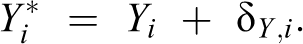
Here, δ _Y,i is the measurement error and is assumed to be independent from all other quantities in the model. An exactly parallel specification is adopted for measurement error in the main explanatory variable.

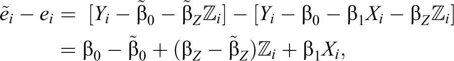
For omitted variable situations, the correct regression model includes an unknown variable or variables, U_i , such that:

Y_{i} = β_{x} X_{i} + β_{z} Z_{i} + β_{u} U_{i} + ε_{i} .

However, the scholar is initially unaware of the identity of the U variable, and so estimates a worse regression, with asterisks added to denote quantities that may be affected by the omission of U:

Y_{i} = β_{x}^{*} X_{i} + β_{z}^{*} Z_{i} + ε_{i}^{*} .

Here, by algebraic substitution, $ε_{i}^{*} = (β_{x} - β_{x}^{*}) X_{i} + (β_{z} - β_{z}^{*}) Z_{i} + β U u_{i} + ε_{i}$ . Of particular note here is the appearance of U in the expression. Because successful regression-based inference requires the error term to be unrelated to the included explanatory variables, whenever U is related with X there will be bias in causal inferences connected with X.⁵ Because such bias is a very common possibility, discovering U and incorporating it appropriately into the model is essentially a precondition for learning about the causal connection between X and Y (for further discussion, see Morgan and Winship 2007:59-86).

When the goal of interest is discovering or testing a hypothesis about a variable on the causal path from the main explanatory variable to the outcome variable, the analysis below will adopt a potential outcomes mediation model (Imai, Keele, and Tingley 2010), generalized along the lines of Freedman’s response schedules concept (2009:94-102) to allow for continuous treatment variables. In this setup, the pathway variable W_i takes on value f_W,i (t) when the causal variable X_i = t. The function f_W,i is case-specific and need not be linear, monotonic, and so on. This function provides a full counterfactual description of what would have happened to the value of W in case i if all else were held constant other than the value of X; any desired causal effect can be calculated for this case by taking the differences among values of this function. Needless to say, this function is usually unknown and is at best difficult to estimate. A second function of the same general kind relates W and X with the outcome variable, Y: g_Y,i (w, t), which characterizes the outcome that would happen in case i if X were set to t and W were set to w. The combination of these two functions specifies the causal path of interest.

The researcher who wants to discover or test hypotheses about W as a step between X and Y needs to select cases where W_i is far from that variable’s mean across the population. Because W is hypothesized to be caused by X and to be a cause of Y, selection techniques that focus on either variable may prove to be helpful.

The last two goals to be considered also make use of the potential outcomes framework for thinking about causation. Here, attention focuses solely on the effect of the main independent variable, X, on the main outcome variable, Y. If X, conceptualized as a metaphorical or literal experimental treatment, is present for case i, then the value of the outcome variable that we observe for that case is Y_i,t ; if all is the same for the case other than that X is absent, then we instead observe Y_i,c . The effect of X on Y for case i is Y_i,t − Y_i,c , a quantity that defines a potentially case-specific causal effect. While this case-specific effect normally cannot be directly observed or easily estimated, it is nonetheless well defined and can be the focus of attention in selecting cases.

In particular, consider a scholar who is interested in tracing the causal process connecting X and Y in a case that has as typical a causal effect as possible. It is natural to represent that goal as entailing the selection of a case for which Y_i,t − Y_i,c is as close as possible to the population average, ${\bar{Y}}_{t} - {\bar{Y}}_{c}$ .

Case study researchers are sometimes interested in discovering the substantive reasons for causal heterogeneity. We will represent this goal as involving a situation in which the size of the causal effect depends on an unknown variable, P. For cases with a large and positive value of P, Y_i,t − Y_i,c also tends to be large and positive; when P is negative, the effect tends to be small. Thus, there is a positive correlation between P and the causal effect of interest. Case selection will be regarded as successfully facilitating the goal of discovering the causes of heterogeneity when the cases chosen have a value of P_i that is at least two standard deviations from its mean.

Finally, when the goal is to reestimate the overall relationship between X and Y based on comparisons across the selected case studies, things are kept as simple as possible. For a paired comparison between cases 1 and 2, which is the design analyzed throughout, the result of the reestimate is taken to be:

\frac{Y_{2} - Y_{1}}{X_{2} - X_{1}} .

This is simply the slope of the line segment connecting the two points. The next section will use these simplified models of case study research goals to argue that deviant and extreme-on-the-independent-variable procedures are usually the best ways to choose cases. First, however, it is essential to review the case selection techniques in question.

Techniques for Choosing Cases

Past discussions of case selection in the social sciences have rarely offered detailed arguments connecting techniques with the kinds of goals discussed above. Lieberman (2005), for example, connects two case selection practices with discovering causal pathways, identifying omitted variables, and improving measurement—but does not argue that either technique is connected with any of these goals in particular. Seawright and Gerring (2008) characterize techniques in broad terms as exploratory or confirmatory and only sometimes connect specific techniques with particular goals. Other authors, including King et al. (1994) and (Fearon and Laitin 2008), justify their case selection advice as a way of avoiding specific threats such as selection or confirmation bias. Thus, for the most part, the state of the debate is one in which a large number of techniques exist, but only fragmentary arguments have been made about the goals that can be achieved by each.

To improve on this situation, a first necessary step is offering a specific definition of each case selection technique. The stylized scenario to be considered here is one in which, before selecting cases, a scholar has carried out a regression analysis in which an outcome of interest, Y, is predicted by a hypothesized cause, X, and generally also a set of control variables, ℤ.⁶ This regression is taken to represent the available knowledge about the relationship in question.⁷ In setting up these regressions, problems of descriptive or causal inference are not fatal. After all, the discussion here presumes that the goal of the case study research is discovery; finding such problems when they exist is thus an objective of the research, rather than an obstacle to it. On the other hand, a subpar regression that does not incorporate the best current descriptive and causal knowledge is likely to produce case studies that rediscover existing knowledge. Thus, it is important to make the regression starting point as good as possible.

While slope estimates are typically the focus of attention in applied regression analysis, other regression-related quantities matter more for case selection. “Fitted values,” typically written as $\hat{Y}$ , reflect the best guess for the score on the dependent variable for each case if for some reason we did not have those scores and only had access to the regression results and the information in X and ℤ. The regression residuals, represented in vector form as e, are the difference between the actual values of Y and the fitted values; these represent the component of the outcome that the regression cannot successfully predict. Cook’s distance scores (Cook and Weisberg 1982) measure the extent to which the overall regression results would change if that one case were deleted from the analysis. A similar score, called the DFBETA (Belsley, Kuh, and Welsch 1980:13), indicates the extent to which a single, selected coefficient would change if one given case were deleted from the analysis.

The case selection techniques discussed in this article are summarized in Table 1 using the notation just mentioned. It is beyond the scope of this analysis to offer a detailed introduction to these techniques; however, a brief review may be helpful. Random case selection involves choosing cases with equal probability from the entire data set (Fearon and Laitin 2008).

Table 1.

Techniques for Choosing Cases.

Selection Rule	Implementation
Random	Select case(s) randomly with equal probability from the entire data set.
Typical	Select case(s) to minimize $\| Y_{i} - {\hat{Y}}_{i} \|$ .
Deviant	Select case(s) to maximize $\| Y_{i} - {\hat{Y}}_{i} \|$ .
Influential	Select case(s) to maximize the DFBETA connected with X_i .
Extreme X	Select case(s) to maximize $\| X_{i} - {\hat{X}}_{i} \|$ .
Extreme Y	Select case(s) to maximize $\| Y_{i} - {\hat{Y}}_{i} \|$ .
Most similar	Select paired case(s) such that X_i, ₁ is “high” and X_i, ₂ is “low” while minimizing the overall difference between ℤ_i,₁ and ℤ_i,₂.
Most different	Select paired case(s) that minimize \|X_i, ₁ − X_i, ₂\| while maximizing the overall difference between ℤ_i,₁ and ℤ_i,₂.
Contrast	Select paired case(s) that maximize \|X_i, ₁ − X_i, ₂\| while minimizing the overall difference between ℤ_i,₁ and ℤ_i,₂.
Pathway	Select case(s) for which $\| Y_{i} - {\hat{Y}}_{i} \|$ is made as much smaller as possible by including X in the regression.

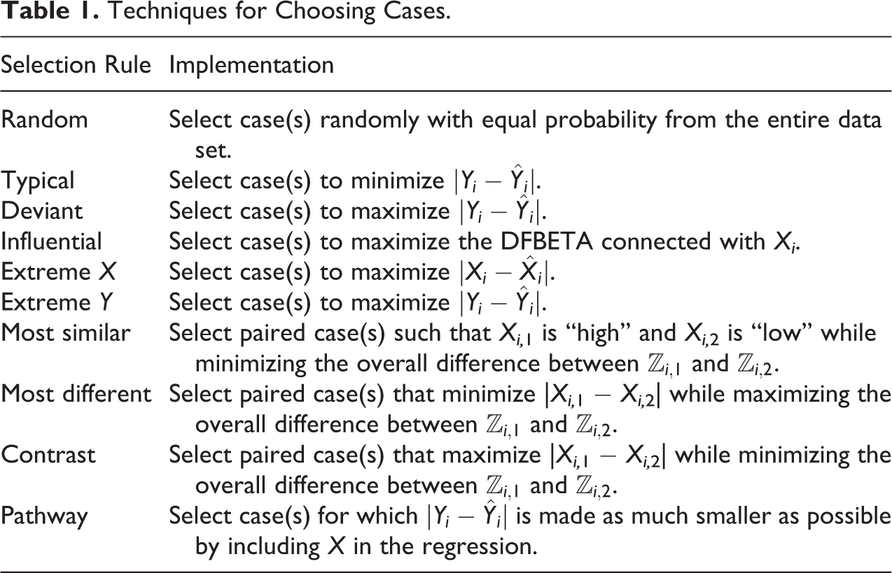
Typical cases are those cases that fit the regression well. Such cases can be identified by selecting those for which the regression’s fitted value is as close as possible to the observed value of the dependent variable. Deviant cases, of course, are just the opposite and can be found by choosing cases for which the fitted value is as far as possible from the observed dependent variable. Extreme cases can be found either on the dependent variable or on the key independent variable of interest; these are simply cases that are as far as possible from the mean on that variable.

Past discussions of influential cases (Seawright and Gerring 2008) focus on those for which Cook’s distance is especially large. Such cases are influential in the obvious sense that they have an unusually large influence on the regression analysis. However, Cook’s distance will sometimes highlight cases that mostly affect coefficients for control variables, rather than the coefficients for the independent variable of central causal interest. A more targeted version of influential case selection uses the DFBETA for the coefficient connected with the most important independent variable.

Three selection rules rely on matching methods (Rubin 2006). Most similar cases involve finding pairs of cases for which the main independent variable differs—that is, it is above some specified threshold for one case and below it for the other—but for which the control variables in ℤ are as similar as possible. Most different cases are pairs in which difference on the independent variable is minimized, but difference on the ℤ variables is maximized. Contrast cases involve a combination of most similar cases and extreme cases on the main independent variable: The pair of cases is selected so as to maximize the difference between them on X while minimizing the difference on the ℤ variables.

Finally, Gerring (2007a) discusses a pathway case approach, in which the analyst chooses those cases for which the regression residual is most reduced in magnitude by the inclusion of the main independent variable of causal interest, in comparison with the residual from a regression model that is identical other than in omitting that main independent variable.

Each of the techniques introduced above has both scholarly advocates and sources of intuitive appeal. Nonetheless, the analysis below will show that deviant cases and extreme cases on the independent variable offer the best chance of making discoveries across a wide range of case study goals. Specifying those goals is the next necessary step in the argument.

Why Deviant and Extreme-on-the-independent-variable Cases Are Usually Best

How should scholars select cases to maximize the probability of case study success? This section provides statistical guidance. Two techniques mostly dominate the others: Selection of cases that are deviant or that are extreme on the main independent variable perform better than the other approaches introduced above across a variety of scenarios. Which of these two options is best depends on the particular objectives of the study. Furthermore, typical case selection is only useful for the goal of tracing causal processes in a case that has a causal effect as close to the population average as possible; for case studies designed to facilitate theoretical discovery, typical cases are generally counterproductive.

Maximizing the Absolute Value of a Sum of Random Variables

Most case selection rules involve maximizing the absolute value of some quantity—that is, picking the cases for which some combination of variables is far from zero. Thus, at various points in the argument below, understanding the application of a given case selection rule to a particular goal involves knowing what it means to maximize the absolute value of a sum of random variables, of the form s_i = |a _1,i + a _2,i|, or possibly with even more elements in the sum. It will be important to know, with case selection rules that choose cases with the highest value of s_i , what will tend to be true of the values of the a_i variables for selected cases. To simplify what is a surprisingly complex topic, cases for which the absolute value of a sum of independent variables is extreme are also relatively likely to have extreme scores on the variables that make up the sum. If some variables in the sum have a higher variance than others, the high-variance variables are especially likely to take on extreme values when the absolute sum is very large, but the low-variance variables also have an above-chance tendency to be extreme. Finally, the probability that any one variable will take on an extreme value in cases where the absolute value of the sum is extreme declines in the number of variables included in the sum. These patterns will turn out to be critically important in understanding the properties of case selection rules.

These summary claims lack a simple proof. Maximizing a sum of absolute values is in general difficult to analyze mathematically (Chadha 2002; Shanno and Weil 1971). A worst-case scenario is possible: The cases with the most extreme values of a _1,i also have extreme values of a _2,i but with the opposite sign. In this scenario, the most extreme cases on s_i will probably not be the most extreme on the a_i variables. However, if the a_i variables are positively correlated, independent, or only weakly negatively correlated, this scenario will be unusual. If the cases with the most extreme values of a _1,i have either average values of a _2,i or extreme values of a _2,i with the same sign, then the set of cases with extreme values of s_i will tend to overrepresent cases with extreme values on one or more of the a_i variables.

An easy way to demonstrate that last statement is via Monte Carlo simulation. Suppose a _1,i and a _2,i are independent standard normal variables. The researcher starts with a population of 100 cases and selects each case in which the absolute value of the sum of those two variables is greater than 2.4, which is approximately the 95th quantile of the distribution of s_i . A Monte Carlo simulation which repeats this process 2,000 times finds that 25 percent of selected cases have values of a _1,i that are two standard deviations or more from the mean—in contrast with only 5 percent of cases in the population as a whole; results are of course identical for a _1,i. Similar results hold for a range of different distributions when the two variables are identically distributed and independent.

When a _1,i has higher variance than a _2,i, then extreme cases on s_i are very likely to have a _1,i > 2. For example, in a Monte Carlo identical to the one discussed in the last paragraph except that the variance of a _1,i is 2 instead of 1, 43 percent of cases where s_i > 2.4 are also cases where |a _1,i| is more than two standard deviations away from its mean. In this simulation, only 14 percent of selected cases have similarly extreme values of |a _2,i|, a substantial decline from the prior simulation although still well above the chance rate of 5 percent.

As the number of a_i variables that are summed together to produce s_i increases, the probability of finding an extreme value on any given a_i variable by choosing cases with extreme values of s_i declines. A Monte Carlo simulation in which s_i is the absolute value of the sum of three, rather than two, standard normal a_i variables sees the proportion of cases with s_i above its 95th quantile that also have |a _1,i| > 2 falls from 25 percent in the two-variable case to 21 percent in the three-variable case. The decline continues, as the number of a_i variables increases. Thus, in summary, unless the quantities of interest have a substantial negative correlation, maximizing the absolute value of the sum of those quantities tends to increase the likelihood of selecting extreme values of the ingredients of the sum, as well. This tendency is crucial for the discussion below, since most case selection techniques involve maximizing the absolute value of a sum of quantities, where the quantity of interest is one element in the sum.

Deviant Cases

The received wisdom regarding case selection is that deviant cases are good for finding omitted variables. This claim turns out to be problematic, but deviant cases can be more broadly useful. This case selection rule also has value as a way of finding sources of measurement error in the dependent variable; in a regression model, such measurement problems are often pushed into the error term and therefore can be discovered via close study of cases with extreme estimated values on that error term.

Furthermore, and perhaps a bit surprisingly, deviant cases can be a useful way to discover new information about causal pathways connecting the main independent with the main dependent variable. This point will be developed formally below, but intuitively the reason is that cases may vary in terms of the size of the causal effect of X on Y. Cases with unusually large effects will often also have unusually extreme values of variables along the causal pathway. Because such cases are causally unusual, they will tend to have large error terms, as well. For the same reason, deviant cases are a useful way of discovering unknown sources of causal heterogeneity.

Let us begin by analyzing the traditional strength of deviant case selection, identifying possibly relevant omitted variables. Deviant case selection, of course, maximizes the absolute value of the estimated error term from a regression, that is, the residual. When there is a relevant omitted variable, as discussed above, the formula for the residual is $e_{i} = d_{i} + γ {\tilde{Z}}_{i}$ , where ${\tilde{Z}}_{i} = Z_{i} - E (Z_{i} | X_{i})$ .

The usual assumption here is that the “true” residual, d_i , is uncorrelated with and perhaps independent of the residualized omitted variable, ${\tilde{Z}}_{i}$ . Selecting cases with a large absolute value of $d_{i} + γ {\tilde{Z}}_{i}$ will increase the probability of selecting cases with large absolute values of both d_i and $γ {\tilde{Z}}_{i}$ —because of the facts about absolute values of sums introduced earlier. The $γ {\tilde{Z}}_{i}$ term is usually related to the omitted variable of interest, Z_i . This means that deviant case selection will increase the probability of finding a relevant omitted variable, unless $γ {\tilde{Z}}_{i}$ is only weakly related to Z_i . This can happen if γ is small, which would mean that Z_i has little or no relationship to Y_i and is thus not an important confounder. Alternatively, deviant case selection can fail if Z_i can be too powerfully predicted by X_i ; thus, unfortunately, this technique will tend to fail if the confounder is strongly related to the main causal variable. Thus, deviant case selection is limited in its ability to help find the most important confounders. It will work for moderate scenarios in which Z_i is quite causally relevant for explaining Y_i but not too closely related to X_i . Simulation results below will explore the relevance of deviant cases for confounders in greater depth, but as a preliminary conclusion, it is obviously unfortunate that the technique degrades in value for the most important confounders.

Turning now to less widely discussed patterns, deviant case selection can also help scholars discover sources of measurement error in the dependent variable. Consider the relationship between the regression residual—whose absolute value is, of course, maximized in deviant case selection—and measurement error in Y. We will write the value of the residual using the econometric identity that ${\hat{Y}}_{i}_{} = ℍ_{i}, Y$ , for a matrix ℍ which is a shorthand for the part of a regression estimate that involves only the independent variables (Greene 2000:263). Then, we can write:

e = Y^{*} - ℍ Y^{*} = Y - ℍ Y + δ_{Y} - ℍ δ_{Y} .

Because the measurement error in Y is assumed to be independent of all of the independent variables in the regression, the last term converges to zero as the number of cases increases. Thus, when there is a large number of cases, the estimated residual converges to the measurement error plus the residual from the regression using Y when measured without error. Choosing e_i to be as far from zero as possible will thus increase the probability of choosing cases with large amounts of measurement error (as well as cases with large residuals in a version of the regression without measurement error, an unwanted side effect). For this reason, deviant case selection can help discover sources of measurement error in the outcome variable.⁸

A further surprising result is that deviant case selection has value for the goal of choosing cases with extreme values on a pathway variable. When treatment assignment is independent of the potential values of Y, conditional on any included control variables, then the residual of a regression of Y on X will in part measure the extent to which a given case has a causal effect of X_i on Y_i that departs from the population average (Morgan and Winship 2007:135). Given the pathway setup introduced above, there are three ways this can arise. First, X_i may have an unusual effect on W_i for this case, which in turn has about the usual effect on Y_i . Second, W_i may have an unusual effect on Y_i for this case. Third, X_i may, in this instance, have an unusual direct effect on Y_i , net of W_i . The second and third of these patterns will be unhelpful in terms of selecting cases with unusual values of W_i ; the first, however, will tend to help. That is to say, because deviant case selection opts for large absolute values of the regression residual, it will increase the probability of choosing cases with large absolute values of the effect of X_i on W_i and of the effect of W_i on Y_i . The first of these two possibilities in turn increases the chance that W will take on atypical values, and thereby facilitates discovery of the causal pathway. Thus, deviant case selection can help in finding out about unknown or incompletely understood causal pathways.

The same basic logic also allows deviant case selection to uncover evidence of unknown sources of causal heterogeneity. Recall that the source to be discovered, P, is correlated with the magnitude of the main causal effect. As argued in the last paragraph, cases for which the effect of X_i on Y_i is quite different from the population average also tend to have regression residuals that are large in absolute value. Hence, selecting based on the regression residual has a reasonable chance of turning up cases for which P_i is far from its mean, and therefore facilitating case study discovery of that source of causal heterogeneity.

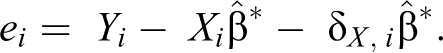
However, there are some goals for which deviant case selection is simply not helpful. Consider first the goal of discovering sources of measurement error in X. We can substitute the measurement error setup in X into the definition of the regression residual:

e_{i} = Y_{i} - X_{i} {\hat{β}}^{*} - δ_{X, i} {\hat{β}}^{*} .

Here, the quality of deviant case selection depends to some extent on the joint distribution of $Y_{i} - X_{i} {\hat{β}}^{*}$ and $δ_{X, i} {\hat{β}}^{*}$ , particularly their relative variance and their correlation. The best-case scenario is one in which the two quantities are negatively correlated and the variance of the measurement error is larger than the variance of $Y_{i} - X_{i} {\hat{β}}^{*}$ —an unusual set of circumstances. Usually, scholars assume that measurement error is independent of systematic variables and is not terribly large in variance. Under those assumptions, deviant case selection will still tend to somewhat increase the probability of choosing cases with extreme values of δ _X,i , because that quantity is part of the expression whose absolute value is maximized. However, the process is relatively indirect because of the combination of measurement error with the true residual.

For some research goals, deviant case selection is outright harmful. Suppose that the goal is to find a case where the effect of X on Y is close to the population average. As discussed earlier, deviant case selection increases the probability of selecting cases with extremely atypical causal effects, and therefore works against this goal.

The second goal for which deviant case selection is counterproductive involves replicating the overall slope estimate. Intuitively, a bivariate slope estimate based on a pair of cases can be described as involving the following fraction:

\frac{(True slope × Difference on X) + Difference on Error Terms}{Difference on X} .

A slope reestimate will work well if the difference between the selected cases in the error term is small relative to the difference on X. Deviant case selection picks cases to maximize the absolute value of the error terms for both cases. If the two cases have error terms with the same sign, this will not distort slope estimates much. However, about half the time, the two cases will have opposite signs, which in combination with large absolute magnitudes means that slope reestimates will be badly off track. Hence, deviant case selection is not a reasonable approach to reestimating the overall slope.

To summarize, deviant cases are valuable for several kinds of discovery: learning about sources of measurement error in the outcome, discovering information about the causal pathway connecting X and Y, and finding out about sources of causal heterogeneity. The technique also has some limited value for discovering confounders. The value of this case selection rule has been underestimated and misunderstood in the literature to date, which has mostly emphasized its potential contribution in terms of omitted variables.

Extreme Cases

There are two variants of the extreme cases strategy: extreme cases on the independent variable, X, and the more frequently discussed extreme cases on Y. This section argues that choosing cases with extreme values of X_i is a valuable and underrated strategy and is more broadly applicable than selecting cases with extreme values of the dependent variable, Y_i . Indeed, I will argue that, for goals where extreme cases on Y can be helpful, deviant cases are often superior.

Consider first the project of discovering sources of measurement error; here, success requires selecting cases in which the variable of emphasis (X or Y) is especially badly measured. Choosing cases as far as possible from the mean on X* (i.e., the X variable measured with error) is equivalent to maximizing the absolute value of X_i + δ _X,i . Once again, cases with an extreme value on the absolute sum of two variables will have a heightened probability of having extreme values on each of those two variables. Hence, extreme case selection on X increases a scholar’s chances at finding cases with a good deal of measurement error.

Obviously, this argument applies equally to the task of finding measurement error on Y using extreme case selection on the outcome variable. However, and perhaps somewhat surprisingly, deviant case selection will typically outperform extreme case selection on the dependent variable for the task of finding measurement error on that variable. The last section showed that, in measurement-error scenarios, choosing deviant cases tends to push to an extreme both the true residual from a regression explaining Y and the measurement error on Y. Extreme case selection, by contrast, selects for extreme values of true Y and of the measurement error.

A comparison of the two methods thus involves contrasting distraction factors, that is, irrelevant quantities that are pushed to an extreme and that potentially distract from maximizing the quantity of interest. The distraction factor for deviant case selection, the true regression residual, has a variance that is by definition less than or equal to the variance of the variable Y measured without error; therefore, deviant case selection generally has a smaller distraction factor than extreme case selection. After all, as mentioned in the section about sums of absolute values, the variable of interest is more responsive to maximizing the absolute value of the sum, as the variance of the other variables in the sum shrinks. Thus, when searching for measurement error in the outcome variable, deviant case selection is better than extreme cases on the dependent variable.

When the goal of case study research is to discover omitted variables, extreme case selection on the dependent variable can have real value. Recall that the residual in the regression of Y on X is partitioned as $e_{i} = d_{i} + γ {\tilde{Z}}_{i}$ . Thus, Y_i can be represented as a sum of three quantities: $\hat{Y} i$ , which represents the predicted value of Y_i , conditional on X_i ; d_i , the portion of the residual that remains unaccounted for after considering the effects of the omitted variable to be analyzed; and $γ {\tilde{Z}}_{i}$ , the effect of an X residualized version of Z_i on Y_i . In a now familiar refrain, we can conclude that selecting cases with extreme values on Y will tend to maximize the absolute value of each of them. While the d_i term is irrelevant, the fitted value of Y will be relevant when the omitted variable matters most. If the omitted variable is independent of the included variables, they are strictly irrelevant; if the omitted variable is related to some included variable, $\hat{Y} i$ will be contaminated by that relationship. In particular, if the omitted variable is substantially related to X—as is the case for the most important confounders—then $\hat{Y} i$ will capture a substantial component of the effect of Z_i on Y_i because much of that effect will be statistically attributed to X_i . Thus, extreme case selection on Y works well when the stakes are highest.

Extreme case selection on X is also a good idea when the stakes are highest. If the omitted variables are not confounders, that is, are independent of the included variables, then extreme cases on X should be altogether unhelpful. After all, X by assumption contains no information about the omitted variables. Obviously, when the omitted variable is correlated with X_i , then the success rate of an extreme case selection rule on X will depend directly on the strength of the correlation. Since omitted variables matter most when they are strong confounders—and therefore substantially related to X, this technique should have an advantage when it matters most.

In contexts where the emphasis in the case study research is on discovering or demonstrating the existence of a pathway variable causally connecting X and Y by selecting cases with extreme values on that pathway variable, extreme case selection on X can be a very strong approach. When the average effect of X on the pathway variable is large, then the average case where X takes on an unusual value will obviously have an unusual value for the pathway variable W. Hence, when the key independent variable is an important cause of the outcome and the pathway of interest captures a large share of the overall effect, extreme case selection on X is a good idea.

Extreme case selection on Y will also work well when the pathway variable, W, explains much or most of the variation in the outcome—because in these contexts, extreme cases on Y are likely to be cases where W is high, as well. Deciding whether extreme case selection on the dependent variable is ever a best approach requires some analytic thought. Suppose that Y takes on an extreme value because W also takes on an extreme value. This can happen in one of the two ways. First, W may take on an extreme value because its cause, X, also takes on an extreme value. In this case, selection on X should be more or less as useful as selection on Y. Second, W may take on an extreme value even though X does not, because of some kind of unobserved uniqueness in the case in question. If this is so, then deviant case selection is likely to pick up the case in question. Either way, whenever extreme case selection on Y is useful for finding pathway variables, it is to be expected that either selection on X or deviant case selection would be about as good.

When scholars wish to discover unknown sources of causal heterogeneity, extreme cases are less useful than deviant cases. In the first place, extreme cases on the independent variable are altogether unhelpful here. After all, the value of X_i should generally tell us little about the causal effect of X_i on Y_i , and in fact the two quantities are usually assumed to be independent.

Extreme cases on Y are more relevant but still not as good as deviant cases. Intuitively, when the effect of X_i for a given case is unusually large or small, and when X_i takes on an unusual value, mathematically Y_i also has to take on an unusual value. Unfortunately, Y_i can also take on an unusual value even when the causal effect for the case is perfectly average—if X_i also takes on a sufficiently unusual value. Deviant case selection deals with this possibility because the residual for case i accounts for the value of X in that case. Thus, deviant case selection captures the good of extreme cases on Y for this goal while also eliminating one scenario in which the latter procedure fails.

For the goal of reestimating the overall slope between Y and X, extreme case selection on X once again a useful approach. Maximizing the difference between selected cases on X_i increases the two systematic components of the slope ratio in equation (1) as much as possible while leaving the error component unaffected, thereby tending to get the right answer. Maximizing the difference between selected cases on Y_i will also be productive, in that it tends to maximize the systematic component of the numerator, and indirectly increases the size of the denominator to the extent that X and Y are correlated. However, this approach will underperform in comparison with extreme case sampling on X because maximizing the difference between selected cases on Y_i also tends to maximize the difference between the selected cases on their error terms.

When the research requires finding a case with a causal effect close to the population average effect, neither variety of extreme case selection is useful. Under the common assumption that values of X_i are independent of treatment effect sizes, extreme values of X_i are exactly as likely to have approximately average causal effects as any other case. On the other hand, cases with extreme values of Y_i are by definition cases that have an extreme value of at least one potential outcome and therefore are more likely to be cases with extreme causal effects than cases with average effects.

Overall, extreme case selection on X is a powerful, underappreciated approach to choosing cases for in-depth analysis. This is a strong approach for discovering measurement error, examining causal pathways, and reestimating overall slopes, and it can also be useful in some omitted-variable scenarios. Case study scholars should seriously consider adding this approach to their applied repertoire.

Random Sampling

The argument so far has shown that deviant and extreme-on-X selection rules can help achieve most of the goals under analysis here; extreme cases on Y have some value but should be less central. The task for the remainder of this section is to much more briefly argue that the remaining set of case selection rules are far less useful.

To begin with, it should be clear that random sampling is never a powerful option for any of the goals considered in this analysis. The reason random sampling is a bad reason to choose cases for case study research is in fact the same as the reason it is a good way to draw survey samples: the law of large numbers. That law tells us that, on average, random sampling will select cases from a given category in proportion with that category’s share of the overall population. But because the cases that constitute success for discovery-oriented case study analysis are by definition the most unusual cases, it will be unusual for random sampling to produce successful case studies.

The main methodological justification for random sampling is that it prevents scholars from selecting cases because those cases are likely to fit the substantive argument of interest (Fearon and Laitin 2008). Yet in fact, any systematic case selection algorithm has this same virtue, and thus there is really no viable justification for randomly selecting case studies.

Typical Cases

Choosing typical cases is also almost always a bad idea. The reasoning is simple: Typical cases are by definition the exact opposite of deviant cases. Whatever deviant case selection tends to maximize, typical case selection tends to minimize. As a consequence, the pattern of strengths and weaknesses for typical cases is more or less a mirror image of those for deviant cases. Specifically, typical case selection tends to reduce scholars’ probability of making discoveries about sources of measurement error, omitted and confounding variables, pathway variables, and unknown sources of causal heterogeneity. However, it is helpful for the replication-oriented goals of studying a case in which the causal effect is as close to the population average as possible and reestimating a regression slope.

Case study methodologists have long shared an intuition that typical case selection should be a good idea. After all, these are the cases that best fit the overall relationships among variables. Yet this is exactly why typical case selection is ineffective when the goal is to discover more about the relationship in question than what can be captured by regression. Simply put, it is hard to learn about problems with a regression by looking at the cases that fit well in that regression.

Influential Cases

Influential case strategies to date involve selecting cases based on their Cook’s distance scores, which effectively combine the deviant case criterion with attention to high-leverage cases. For a bivariate regression of Y on X, cases have high leverage if and only if they have unusually high or low values of X_i relative to the rest of the sample; hence, in this simple context, influential case selection is a straightforward combination of deviant case selection, discussed above, and selection of cases with extreme values on X_i . Such a combination may be helpful for discovering pathway variables, because it will tend to push the pathway variable toward extreme values from both directions—that is, cases with high Cook’s distance scores will tend to have unusual values of both X_i and Y_i and therefore are likely to have unusual values of W_i .

The issue becomes more complex when the regression of interest is multivariate. In such situations, leverage scores reflect a complex weighted mixture of cases’ degree of extremeness on X_i and on the various control variables included in the model. This feature waters down the focus and makes influential case selection less appropriate for the various goals considered in this article. Hence, for case selection in the context of multivariate models, the Cook’s distance influential cases strategy is likely to be suboptimal. The alternative influential cases strategy of selecting for high values of DFBETA for the X coefficient recreates the relevant virtues of the bivariate Cook’s distance statistic for models with control variables and thus should be a fairly effective way of finding pathway variables.

Most Similar, Most Different, and Contrast Cases

The most similar cases selection rule, using matching techniques to quantify similarity, is not an advisable approach to case selection for any of the case study goals considered in this article. Matching chooses cases that are different on X_i but as similar as possible on a set of conditioning variables ℤ_i. Yet that set of conditioning variables need not have a connection with the quantities of central interest for case study goals.

Consider measurement error. By standard assumption, ℤ_i is independent of error in either X_i or Y_i . Hence, a most similar cases selection rule for measurement error on X has traction only to the extent that the treatment and control cases selected by the rule reflect extreme scores on an underlying continuous variable X_i ; the attention to ℤ_i is wasted. When there is measurement error on Y, both X and ℤ are by the usual assumptions irrelevant, so most similar cases are useless. For omitted variables, the problem is the same: ℤ is usually assumed to be independent of the omitted variable and so uninformative. Because causal pathways between X and Y are usually intended to be insulated from other causal factors, any unknown pathway variable should also be independent of ℤ; once again, matching should be unhelpful. Most similar case selection may help reestimate the overall slope, given that it assures at least some difference between the selected cases on X_i and may reduce the difference on error terms to the extent that the variables in ℤ are selected skillfully; however, in practice, maximizing the difference between cases on X_i can outperform the most similar case design, as will be seen in the simulations below. Finally, confounding variables are generally assumed to be unconnected with the magnitude of the causal effect for the case, so choosing most similar cases does nothing to help with the tasks of finding cases with causal effects close to the population average or discovering sources of causal heterogeneity.

This widely discussed case selection strategy, like typical cases, turns out to be much less useful than its prevalence in the literature and in practice would suggest. For both case selection techniques, the problem seems to be an insufficiently reflective imitation of regression-type causal inferential practices. In this case, the argument seems to be that control variables may solve some kinds of problems in regression, so for that reason they are used in case selection for qualitative research. Yet in fact, case study methods do not work by a logic of estimating conditional effects, and so control variables do not perform in the same way as in regression. It seems plausible that they do not in fact help at all; if they do, some new and careful argument to that end is needed.

Most case study methodologists warn against most different case selection, and a simple argument suffices to all but rule them out. As with most similar cases, most different case selection depends almost entirely on the specification of the ℤ variables, which typically have little relationship with the quantities of interest in the scenarios considered here. Hence, there is little to be gained by selecting the least matched cases.

Finally, the contrast cases approach involves selecting cases that maximize a combination of the criteria used in two other sampling rules: extreme cases on X and most similar cases. The properties of this approach are thus a mix of the two. For most goals, this makes the contrast cases sampling rule a degraded version of the extreme-cases-on-X design, since the most similar cases sampling rule rarely adds much to the process and attention to matching therefore coarsens the quality of the selected cases. However, this may be a very good approach for reestimating the overall slope between X and Y because it subtracts out confounders that may matter for such a task and tends to maximize the variance in X.

Pathway Cases

One last case selection rule deserves a brief discussion: The pathway case selection rule discussed by Gerring (2007a), which, as a newer case selection procedure, has not been widely discussed. Choosing pathway cases involves choosing the cases whose residuals are most reduced in magnitude by including X in the regression, in comparison with an otherwise identical model excluding X. The key quantity here is:

{\tilde{e}}_{i} - e_{i} = [Y_{i} - {\tilde{β}}_{0} - {\tilde{β}}_{Z} ℤ_{i}] - [Y_{i} - β_{0} - β_{1} X_{i} - β_{Z} ℤ_{i}] = β_{0} - {\tilde{β}}_{0} + (β_{Z} - {\tilde{β}}_{Z}) ℤ_{i} + β_{1} X_{i},

where the quantities with tildes come from a restricted version of the regression that drops the variable X. In the special case that X has mean 0 and has no information about⁹ ℤ, this simplifies to β₁ X_i and will thus select exactly the same cases as an extreme-cases-on-X strategy.¹⁰ When X does contain information about ℤ, this rule modifies extreme-cases-on-X selection by adding a kind of covariance adjustment based on the relationships among X, ℤ, and Y as well as the case’s value on the ℤ variables. This covariance adjustment involves quantities that do not appear in any of the formulas connected with the goals of case study research considered here and thus may involve attention to an undesired quantity. On the other hand, the adjustment may sometimes reduce the variance of some irrelevant quantities in the selection formula. While the trade-off between these two considerations will depend on the parameters of the situation of interest, the pathway case rule will usually perform about the same as extreme case selection on X.

This section has argued that case selection should usually focus either on extreme cases on the independent variable or on deviant cases. These two case selection procedures are sensitive to the kinds of discoveries that case study researchers are most likely to pursue in multimethod contexts: discoveries about sources of measurement error, variables that constitute causal pathways from the independent to the dependent variable, sources of causal heterogeneity, and confounding variables. In particular, an extreme cases selection rule on X is valuable for identifying omitted variables, for identifying sources of measurement error on the X variable, for discovering pathway variables or testing claims about such variables, and for reestimating the overall slope. Deviant case selection is useful for finding pathway variables, exploring sources of causal heterogeneity, and discovering reasons for measurement error on the Y variable.

In contrast, some popular case selection rules are much less useful for these goals. Case selection strategies that pay attention to control variables, such as most similar, most different, contrast, and pathway cases, are not usually optimal. Whereas control variables can be essential for some quantitative approaches to causal inference, they offer little help in dealing with measurement quality, discovering omitted variables, finding potential causal pathways, and other central case study goals.

Finally, the popular strategy of typical case selection is not helpful as a way of discovering new things about cases, and indeed works well only for finding cases whose causal effects closely mirror the average for the population as a whole. Indeed, even this goal deserves further thought. Such cases will—by construction—be those where estimates from cross-case inferential techniques such as regression are most accurate. At the same time, they are cases that are least likely, for reasons discussed above, to produce new discoveries about causation or measurement. What, then, is the value of such case studies? The issue deserves clarification if a defense of the common practice of choosing typical cases is to be mounted.

The Fit Between Techniques and Goals: Simulations

Of course, the results above involve quite simple stylized scenarios for each potential research goal, and some analysis of the sensitivity of the results is worthwhile. For example, the relationship between Y and X is represented as bivariate, with no control variables entered into the analysis. In general, adding control variables changes some details of the results above but not the overall patterns; simulations demonstrating this claim are available from the author upon request. This section will focus on limiting conditions noted in the analysis above for techniques’ value in finding omitted and pathway variables.

For each scenario, real data are randomly modified to capture the scenario of interest. Then case selection is carried out, and success or failure in terms of facilitating the designated goal for case study research is recorded. This process is repeated a large number of times, generating Monte Carlo results regarding the propensity for success of each case selection rule with respect to a given goal. Full details about the simulations, as well as replication code, are available from the author upon request.

The simulation study analyzes a data set focused on Latin American presidential elections, including every such election between 1980 and 2002, for a total of 84 elections, of which 19 are omitted from the analysis due to missing data. The dependent variable is the first difference in the vote share of the incumbent president’s party in the election; independent variables are the largest opposition party’s vote share in the prior election, a dummy variable indicating whether that largest opposition party has fielded a presidential candidate in the new election, the average inflation rate over the presidential term, the average growth rate over that term, and the country’s per capita gross domestic product during the year of the current election. All vote shares are transformed by the logit function, such that they range in theory from negative infinity to positive infinity; otherwise, the analysis is a standard ordinary least squares (OLS) regression.¹¹

First, in the discussion above of omitted variables, it emerged that the desirability of various techniques depends on the strength of the omitted variable’s relationship to the main explanatory variable and to the outcome. Deviant case selection may work when the confounder is relatively weakly related to X but strongly related to Y, while the value of extreme case selection on either the cause or the outcome quite obviously depends on the strength of the relationship between the confounder and the variable used for selection. It remains unclear, however, how these techniques and others perform across the range of possible strengths of confounding.

To explore this issue, the first set of simulations below generates artificial confounders with varying degrees of statistical connection to the X and Y variables. Specifically, the confounder is generated by a linear combination of the observed value of X—assigned a weight strictly between 0 and 1—and a normal variable with mean and standard deviation equal to that of X—assigned a weight that is 1 minus the weight for the observed value of X. Thus, as the X weight approaches 1, the confounder and X become increasingly related.

A similar process is carried out to simulate new values of Y. Specifically, values are generated by, first, regressing Y on X and a set of control variables. The fitted value of Y from that regression is then added to a linear combination of the residual from that regression and the confounder—with a weight mixing the two quantities as above. As the Y weight approaches 1, the variance in Y that is unrelated to the observed variables becomes increasingly related to the confounder, and therefore the confounder becomes increasingly strong.

The results, shown in Figure 1, suggest that the undesirable regression adjustment involved in deviant cases—which removes any component of the confounding variable that is correlated with X or any other included variable—destroys the value of the technique in the vast majority of situations. In fact, the simulations find that deviant cases are only best for extremely weak confounders; for situations in which the X and Y weights are both below 0.1, which are not displayed here, deviant cases are best. However, discovering such weak confounders is of little practical inferential value.

Figure 1.

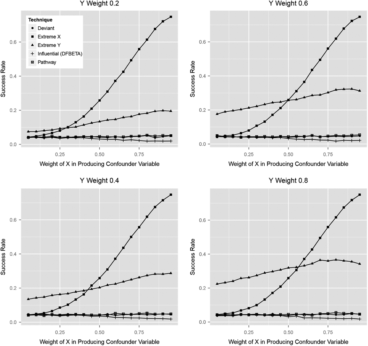
Confounder.

Instead, important confounders are most likely to be discovered with extreme cases on Y and especially on X. There is an asymmetry between the two selection techniques because the simulation assumes that Y has multiple causes and that the confounder is not equally related to all of them. Under this assumption, extreme cases on X emerge as clearly superior for finding the strongest and most important confounders. This result will degrade if the confounder is the main or—at the limit—only true cause of Y, such that it necessarily has a confounding role for every control variable in the regression as well as X. In this scenario, extreme cases on X and on Y will be equally valuable for finding the most important confounders, and extreme cases on Y will win out for confounders of moderate importance. More generally, both flavors of extreme case selection have value here, but extreme cases on X can be the most sensitive to particularly powerful confounders.

Second, the analysis of pathway variables reveals a similar scenario in which the relative value of various techniques depends on the strength of the pathway variable’s connections to both X and Y. To capture this situation, a pathway variable is simulated as a linear combination of a normal random variable with mean and standard deviation equal to that of X and the observed value of X multiplied by a case-specific causal effect that is normally distributed with a mean and standard deviation of 1. Thus, the stronger the X weight, the more the pathway variable consists of the effect of X.

Then, an outcome variable is simulated by subtracting out the estimated effect of X and then adding in a linear combination of X and the simulated pathway variable—each multiplied by the estimated effect times a random case-specific causal component that is normally distributed with a mean and standard deviation of one. As the Y weight approaches 1, the pathway variable comes closer to accounting for the whole effect of X on Y.

The results for pathway variables, shown in Figure 2, are simple and fit cleanly with the expectations developed in the analytic section. Extreme case selection on X is the best option when the pathway variable is weakly connected to the outcome variable, Y. Of course, the performance of this case selection rule does not depend at all on the outcome, and its success rate is not affected by the relationship between the pathway variable and Y. Extreme cases on the cause are best when the pathway only accounts for a portion of the effect of the treatment on Y because nothing else works especially well in that situation.

Figure 2.

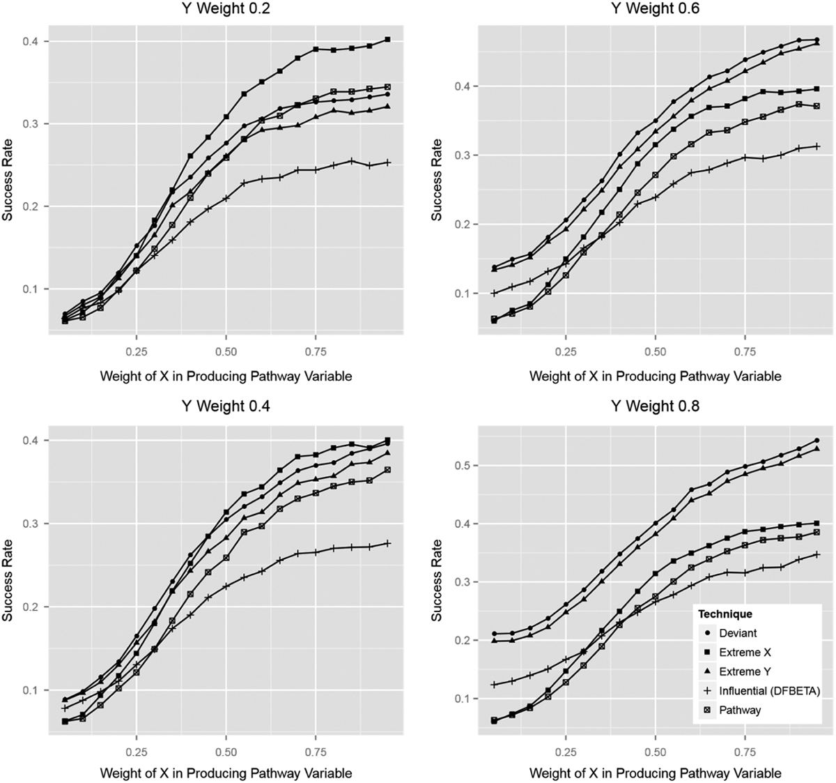
Pathway variable.

As the pathway variable captures a greater share of the overall effect of the treatment on the outcome, deviant- and extreme-on-Y approaches to case selection improve to the point that they beat extreme cases on X—ultimately by a substantial margin. As expected, deviant cases are consistently, if not substantially, better than extreme cases on Y. Indeed, for causal pathways that are powerfully connected to both X and Y, deviant case selection meets the two standard deviation rule for successfully half the time. Thus, the simulations support the finding that deviant cases are best for major causal pathways and that extreme cases on X are an acceptable fallback when the existing pathways are expected to be multiple and fragmentary.

It bears mention that the intended goal of selecting pathway cases is exactly to find pathway variables in the sense discussed here (Gerring 2007a:238-39). Hence, it is striking that pathway case selection does not perform best at this goal in any of the simulations reported here. Instead, the success rate for pathway cases tracks, but is consistently lower than, the results for extreme cases on X.

These two simulations focus on the most intrinsically causal as well as the most parameter-dependent findings from this article’s analysis, and the results emphasize the distinctive value of deviant and extreme-on-X case selection. One or the other of these techniques is the most efficient way to discover confounders or variables that form part of the causal pathway from the treatment to the outcome. When one considers as well the value of these variables in discovering sources of measurement error and causal heterogeneity, the pivotal role of these techniques becomes clear.

Conclusions

The overall argument of this article, supported by both the analytic section and the simulations above, is that deviant cases and extreme cases on X are the best ways to choose cases for close analysis when the goal is discovery. Deviant cases are an efficient means of discovering sources of measurement error, information about causal pathways, and sources of causal heterogeneity. Extreme cases on X are useful for inquiring into sources of measurement error on the treatment variable and discovering the most important and powerful confounding variables as well as for the less justifiable objective of replicating the original slope estimate.

Other case selection techniques perform less well and, in some cases, are categorically unhelpful. Random sampling—both in relative and in absolute terms—performs poorly. Most similar and most different designs are substantially outperformed by other approaches. The pathway cases design is outperformed for its central intended purpose of discovering causal pathways by extreme cases on X for pathway variables that explain only a fraction of the overall treatment effect and by deviant cases selection for variables that are closer to a comprehensive account of the causal effect of interest. Similarly, the contrast cases design is dominated by selecting extreme cases on X. Finally, and perhaps somewhat surprisingly, deviant case selection or extreme case selection on X usually achieves the same goals more efficiently than the frequently discussed and applied approach of selecting extreme cases on the dependent variable. These techniques stand in need of a different kind of justification if they are to continue in use.

A concluding note of caution is in order. The analysis and simulation study above are both constructed around the assumption that the model for the relationships among the dependent, independent, and perhaps control variables is an OLS regression. While some of the conclusions reached here will no doubt generalize to nonlinear models, and perhaps also to semi- and nonparametric approaches such as matching, it is by no means certain that all of this article’s findings will be general in this sense. Likewise, additional analysis will be needed to know how best to select cases when the goal is to interact with a quantitative natural experiment using more complex forms of statistical analysis (e.g., instrumental variables or contemporary approaches to the analysis of regression-discontinuity designs). These cautions notwithstanding, the arguments above do apply in an important context: case studies intended to interact with findings reached using the very common technique of OLS regression.

Footnotes

Declaration of Conflicting Interests

The author(s) declared no potential conflicts of interest with respect to the research, authorship, and/or publication of this article.

Funding

The author(s) received no financial support for the research, authorship, and/or publication of this article.

Notes

References

Baccini

Leonardo

Urpelainen

Johannes

. 2014. “International Institutions and Domestic Politics: Can Preferential Trading Agreements Help Leaders Promote Economic Reform?” Journal of Politics 76:195–214.

Belsley

D. A.

Kuh

Welsch

R. E.

. 1980. Regression Diagnostics: Identifying Influential Data and Sources of Collinearity. New York: Wiley.

Bennett

Andrew

Elman

Colin

. 2006. “Qualitative Research: Recent Developments in Case Study Methods.” Annual Review of Political Science 9:455–76.

Bowles

Samuel

Gintis

Herbert

. 2002. “The Inheritance of Inequality.” Journal of Economic Perspectives 16:3–30.

Bowman

Kirk

Lehoucq

Fabrice

Mahoney

James

. 2005. “Measuring Political Democracy: Case Expertise, Data Adequacy, and Central America.” Comparative Political Studies 38:939–70.

Cameron

A. Colin

Trivedi

Pravin K.

. 2005. Microeconometrics: Methods and Applications. Cambridge, UK: Cambridge University Press.

Chadha

S. S.

2002. “Fractional Programming with Absolute-value Functions.” European Journal of Operational Research 141:233–38.

Collier

David

Brady

Henry E.

Seawright

Jason

. 2004. “Sources of Leverage in Causal Inference: Toward an Alternative View of Methodology.” Pp. 229–66 in Rethinking Social Inquiry: Diverse Tools, Shared Standards, edited by Brady

Henry E.

Collier

David

. Lanham, MD: Rowman and Littlefield.

Collier

David

Mahoney

James

. 1996. “Insights and Pitfalls: Selection Bias in Qualitative Research.” World Politics 49:56–91.

10.

Cook

R. Dennis

Weisberg

Sanford

. 1982. Residuals and Influence in Regression. New York: Chapman and Hall.

11.

Coppedge

Michael

. 1999. “Thickening Thin Concepts and Theories: Combining Large N and Small in Comparative Politics.” Comparative Politics 31:465–76.

12.

Dunning

Thad

. 2012. Natural Experiments in the Social Sciences: A Design-based Approach. Cambridge, UK: Cambridge University Press.

13.

Fearon

James D.

Laitin

David D.

. 2008. “Integrating Qualitative and Quantitative Methods.” Pp. 300–18 in The Oxford Handbook of Political Methodology, edited by Brady

Henry E.

Box-Steffensmeier

Janet

Collier

David

. New York: Oxford University Press.

14.

Flyvbjerg

Bent

. 2006. “Five Misunderstandings about Case-study Research.” Qualitative Inquiry 12:219–45.

15.

Freedman

David A.

2009. Statistical Models: Theory and Practice. Rev. ed. Cambridge, UK: Cambridge University Press.

16.

George

Alexander L.

Bennett

Andrew

. 2004. Case Studies and Theory Development in the Social Sciences. Cambridge, MA: MIT Press.

17.

Gerring

John

. 2004. “What Is a Case Study and What Is it Good For?” American Political Science Review 98:341–54.

18.

Gerring

John

. 2007a. “Is There a (Viable) Crucial-case Method?” Comparative Political Studies 40:231–53.

19.

Gerring

John

. 2007b. “The Mechanismic Worldview: Thinking Inside the Box.” British Journal of Political Science 38:161–79.

20.

Glynn

Adam N.

Ichino

Nahomi

. 2015. “Using Qualitative Information to Improve Causal Inference.” American Journal of Political Science 59:1055-71.

21.

Greene

William H.

2000. Econometric Analysis. 4th ed. Upper Saddle River, NJ: Prentice Hall.

22.

Huber

John D.

Stephens

Evelyne Huber

. 2012. Democracy and the Left: Social Policy and Inequality in Latin America. Chicago: University of Chicago.

23.

Imai

Kosuke

Keele

Luke

Yamamoto

Teppei

. 2010. “Identification, Inference and Sensitivity Analysis for Causal Mediation Effects.” Statistical Science 25:51–71.

24.

King

Gary

Keohane

Robert O.

Verba

Sidney

. 1994. Designing Social Inquiry: Scientific Inference in Qualitative Research. Princeton, NJ: Princeton University Press.

25.

Kreuzer

Marcus

. 2010. “Historical Knowledge and Quantitative Analysis: The Case of the Origins of Proportional Representation.” American Political Science Review 104:369–92.

26.

Lieberman

Evan S.

2003. Race and Regionalism in the Politics of Taxation in Brazil and South Africa. Cambridge, UK: Cambridge University Press.

27.

Lieberman

Evan S.

2005. “Nested Analysis as a Mixed-method Strategy for Comparative Research.” American Political Science Review 99:435–52.

28.

Lijphart

Arend

. 1971. “Comparative Politics and the Comparative Method.” American Political Science Review 65:682–93.

29.

Lijphart

Arend

. 1975. “II. The Comparable-cases Strategy in Comparative Research.” Comparative Political Studies 8:158–77.

30.

Morgan

Stephen L.

Winship

Christopher

. 2007. Counterfactuals and Causal Inference: Methods and Principles for Social Research. Cambridge, UK: Cambridge University Press.

31.

Peterson

Susan

. 1995. “How Democracies Differ: Public Opinion, State Structure, and the Lessons of the Fashoda Crisis.” Security Studies 5:3–37.

32.

Plumper

Thomas

Troeger

Vera E.

Neumayer

Eric

. 2010. “Case Selection and Causal Inference in Qualitative Research.” Unpublished Manuscript.

33.

Poteete

Amy R.

Janssen

Marco A.

Ostrom

Elinor

. 2010. Working Together: Collective Action, the Commons, and Multiple Methods in Practice. Princeton, NJ: Princeton University Press.

34.

Ragin

Charles C.

1987. The Comparative Method: Moving Beyond Qualitative and Quantitative Strategies. Berkeley: University of California.

35.

Ragin

Charles C.

2000. Fuzzy-set Social Science. Chicago: University of Chicago.

36.

Ragin

Charles C.

2004. “Turning the Tables: How Case-oriented Research Challenges Variable-oriented Research.” Pp. 123–38 in Rethinking Social Inquiry: Diverse Tools, Shared Standards, edited by Brady

Henry E.

Collier

David

. Lanham, MD: Rowman and Littlefield.

37.

Rogowski

Ronald

. 2004. “How Inference in the Social (but Not the Physical) Sciences Neglects Theoretical Anomaly.” Pp. 76–83 in Rethinking Social Inquiry: Diverse Tools, Shared Standards, edited by Brady

Henry E.

Collier

David

. Lanham, MD: Rowman and Littlefield.

38.

Rubin

Donald B.

2006. Matched Sampling for Causal Effects. Cambridge, UK: Cambridge University Press.

39.

Rueschemeyer

Dietrich

Stephens

Evelyne Huber

Stephens

John D.

. 1992. Capitalist Development and Democracy. Chicago: University of Chicago Press.

40.

Schweller

Randall L.

1992. “Domestic Structure and Preventative War: Are Democracies More Pacific?” World Politics 44:235–69.

41.

Seawright

Jason

. 2012. Party-system Collapse: The Roots of Crisis in Peru and Venezuela. Stanford, CA: Stanford University Press.

42.

Seawright

Jason

Gerring

John

. 2008. “Case Selection Techniques in Case Study Research: A Menu of Qualitative and Quantitative Options.” Political Research Quarterly 61:294–308.

43.

Shanno

David F.

Weil

Roman L.

. 1971. “Technical Note—“Linear” Programming with Absolute-value Functionals.” Operations Research 19:120–24.

44.

Small

Mario Luis

. 2011. “How to Conduct a Mixed Methods Study: Recent Trends in a Rapidly Growing Literature.” Annual Review of Sociology 37:57–86.

45.

Ziblatt

Daniel

. 2009. “Shaping Democratic Practice and the Causes of Electoral Fraud: The Case of Nineteenth-century Germany.” American Political Science Review 103:1–21.