The Difference Between Instability and Uncertainty: Comment on Young and Holsteen (2017)

Abstract

Young and Holsteen (YH) introduce a number of tools for evaluating model uncertainty. In so doing, they are careful to differentiate their method from existing forms of model averaging. The fundamental difference lies in the way in which the underlying estimates are weighted. Whereas standard approaches to model averaging assign higher weight to better fitting models, the YH method weights all models equally. As I show, this is a nontrivial distinction, in that the two sets of procedures tend to produce radically different results. Drawing on both simulation and real-world examples, I demonstrate that in failing to distinguish between numerical variation and statistical uncertainty, the procedure proposed by YH will tend to overstate the amount of uncertainty resulting from variation across models. In standard circumstances, the quality of estimates produced using this method will tend to be objectively worse than that of conventional alternatives.

Keywords

model averaging model uncertainty model robustness model selection multimodel inference

Introduction

Young and Holsteen (2017)—YH hereafter—introduce methods for dealing with the uncertainty that inevitably results from using multiple models to estimate a single parameter. In making their argument, YH go to great lengths to distinguish their approach from traditional forms of model averaging. The purpose of this comment is to further clarify the difference between these two sets of procedures, both of which provide a set of tools for depicting the distribution of estimates across multiple models. While the YH approach draws on the same basic framework as more conventional forms of model averaging, the two methods differ in how they weight the results of the underlying models. Traditional forms of model averaging typically weight models on the basis of fit, with better fitting models tending to receive more weight. This is true for both Bayesian and non-Bayesian methods. In contrast, the YH procedure treats all models the same, regardless of how well the models in question fit the data. This has substantial implications for the results, especially when it comes to the assessment of statistical uncertainty.

As I show, the weighting mechanism matters insofar as it affects the rate at which numerical variation in the observed parameter estimates is converted to statistical uncertainty. When all models are weighted equally, as is the case with the YH method, numerical variation and statistical uncertainty are one in the same. As the distribution of weights becomes increasingly concentrated, the rate at which numerical variation is converted into statistical uncertainty declines. This means that so long as some models fit better than others, the results produced using the YH method will tend to diverge from those produced using traditional forms of model averaging, with the degree of divergence depending on the extent to which one model tends to outperform all others. These patterns are evident in real-world applications, including the examples considered by YH. As expected, the estimated level of statistical uncertainty produced using the YH method is much higher than what we would get were we to use standard forms of model averaging.

On its face, the choice of whether or not to weight on the basis of fit seems like a matter of preference. This is not the case. The use of weights is integral to the process of statistical inference and is easily justified in terms of basic probability theory. Using simulation, I show that in the absence of orthogonal predictors, the YH method is generally ill-equipped to speak to the characteristics of the data generating process, as evidenced by the propensity to produce intervals that are simultaneously too wide, as well as off-center. So while the flexibility of the method is undoubtedly appealing, it comes at a steep cost. Fortunately, the majority of the procedures proposed by YH have direct analogs in the literature on model averaging.

The Mortgage Example Revisited

The difference between the YH approach and traditional forms of model averaging can be illustrated using a simple example. Here, I draw on the mortgage lending data used by YH. Following their lead, I use linear regression to examine the relationship between gender and the probability of being approved for a mortgage. For the purposes of this particular example, I consider just three controls: martial status, race, and whether or not an applicant was denied personal mortgage insurance. While there are 2,360 observations with complete data on these variables, I focus on the 2,355 observations used by YH. The results are shown in Table 1, which depicts results across the entire model space. When it comes to drawing conclusions, the standard approach is to emphasize the full model, the assumption being that the full model represents a closer approximation to the truth than the simple bivariate model from which we often begin. In most cases, uncertainty in the effect of interest is quantified solely in terms of the standard error, which is typically interpreted in terms of the uncertainty associated with random sampling. Looking at the results in Table 1, it is evident that estimates can also vary considerably across models.

Table 1.

Linear Regression of Loan Status on Select Covariates.

Variable	(1)	(2)	(3)	(4)	(5)	(6)	(7)	(8)
Female	−0.18	2.77	2.49	5.12**	0.06	2.75	2.37	4.79**
Female	(1.63)	(1.79)	(1.62)	(1.77)	(1.53)	(1.67)	(1.52)	(1.66)
Married		5.97***		5.40***		5.44***		4.97***
Married		(1.49)		(1.46)		(1.40)		(1.37)
Black			−19.25***	−18.98***			−16.68***	−16.44***
Black			(1.89)	(1.89)			(1.78)	(1.78)
Denied mortgage insurance					−81.31***	−80.95***	−77.98***	−77.70***
Denied mortgage insurance					(4.45)	(4.44)	(4.39)	(4.38)
Constant	88.23***	83.98***	90.39***	86.52***	89.81***	85.92***	91.61***	88.04***
Constant	(0.75)	(1.30)	(0.76)	(1.30)	(0.71)	(1.22)	(0.72)	(1.22)
N	2,355	2,355	2,355	2,355	2,355	2,355	2,355	2,355

*p < .05. **p < .01. ***p < .001.

Consider, for example, the difference between the bivariate model and the full model. In the case of the former, the parameter estimate associated with gender is −0.18, suggesting that the percentage of female mortgage applicants who are approved for a loan is 0.18 percentage points lower than that of male applicants. In the case of the latter, however, the parameter estimate associated with gender is 4.79, suggesting that, on average, the probability of a female applicant being approved for a loan is actually 4.79 percentage points higher than that of an otherwise comparable male. The estimated effect of gender appears even larger if we ignore whether or not applicants were denied mortgage insurance in the past. In most cases, however, the estimated effect of gender tends to be more modest, lying between 2.37 and 2.77 in four of the eight models. As YH correctly note, our assessment of the relationship between gender and the probability of being approved for a mortgage is sensitive to the choice of controls, with race and marital status emerging as the most influential. This type of variation inevitably raises questions about the idea of committing to any one estimate in particular.

What is to be done? As is the case with model averaging, the YH procedure attempts to quantify the degree of uncertainty resulting from variation in the value of parameter estimates across models. Toward this end, the two sets of procedures draw on a common framework. Given a set of J models, we calculate the mean estimate:

\bar{b} = \sum_{j} ω_{j} b_{j},

and the total variance

v_{t} = \sum_{j} ω_{j} s_{b_{j}}^{2} + \sum_{j} ω_{j} {(b_{j} - \bar{b})}^{2},

where b_j refers to the estimated value of the parameter of interest b associated with model j, with the estimated sampling variance given by $s_{b_{j}}^{2}$ . As equation (2) suggests, the estimated total variance v_t can be decomposed into two distinct parts. Following naturally from the notion of sampling variance in the context of a single model, the mean estimated sampling variance ${\bar{v}}_{s} = \sum_{j} ω_{j} s_{b_{j}}^{2}$ is used to represent the variance in b_j due to switching samples. In contrast, the estimated modeling variance $v_{m} = \sum_{j} ω_{j} {(b_{j} - \bar{b})}^{2}$ is used to represent the variance in b_j due to switching models. The term ω_j can be thought of as a weight depicting the relative contribution of model j. Weights are normalized such that $\sum_{j} ω_{j} = 1$ .

For any given model j, we thus need to calculate three quantities—b_j, $s_{b_{j}}^{2}$ , and ω_j. Values for b_j and $s_{b_{j}}^{2}$ can be calculated in the usual way. This leaves ω_j. Traditional forms of model averaging allow the value of ω_j to vary from one model to the next. While the exact procedure differs depending on the method, weights are typically derived as follows:

ω_{j} = \frac{L_{j}^{*} τ_{j}}{\sum_{j} L_{j}^{*} τ_{j}},

where L* refers to some form of penalized likelihood and τ_j refers to the prior probability assigned to model j. In most cases, L* refers to either a marginal likelihood or some approximation thereof, with $L_{j}^{*} = exp (- 0.5 \times {BIC}_{j})$ being among the most popular (see Raftery 1995). Keeping in mind that models are penalized according to size with larger model receiving a larger penalty, the basic intuition is that better fitting models are assigned a higher weight and thus have more influence on the results. In contrast, YH assume a priori that $ω_{j} = 1 / J$ for all models. The resulting estimates can thus be interpreted as simple unweighted averages.

To see how model averaging and the YH procedure work in practice, consider the results shown in Table 2, which compares the results of model averaging using the Bayesian information criterion (BIC) to results using the YH procedure.¹ For each model, we see the estimated effect of gender b_j, along with the estimated sampling variance $s_{b_{j}}^{2}$ of the estimate in question. We also see the log likelihood LL_j, which is used to calculate the BIC for model j, with ${BIC}_{j} = - 2 {LL}_{j} + k_{j} log (N)$ , where k_j refers to the number of parameters in model j (including the residual standard error) and N refers to the sample size which, in this case, is equal to 2,355. For the purpose of computing model-specific weights, it is often easier to work with the difference $Δ {BIC}_{j} = {BIC}_{j} - {BIC}_{max}$ , where BIC_j refers to the BIC associated with model j and BIC_max refers to the maximum BIC observed across all models. Replacing BIC_j with ΔBIC_j, the approximate marginal likelihood $L_{j}^{*} = exp (- 0.5 \times Δ {BIC}_{j})$ serves as a penalized measure of fit.

Table 2.

Calculations for Multimodel Summaries.

							Bayesian Information Criterion (BIC)				Young-Holsteen Method
Model	b_j	$s_{b_{j}}^{2}$	LL_j	BICj	Δ BICj	$L_{j}^{*}$	ω_j	ω_jb_j	$ω_{j} s_{b_{j}}^{2}$	$ω_{j} {(b_{j} - \bar{b})}^{2}$	ω_j	ω_jb_j	$ω_{j} s_{b_{j}}^{2}$	$ω_{j} {(b_{j} - \bar{b})}^{2}$
1	−0.18	2.67	−11,522.923	23,069.138	388.018	0.000	.000	−0.000	0.000	.000	.125	−0.022	0.334	0.909
2	2.77	3.19	−11,514.918	23,060.892	379.772	0.000	.000	0.000	0.000	.000	.125	0.346	0.399	0.008
3	2.49	2.63	−11,472.298	22,975.654	294.534	0.000	.000	0.000	0.000	.000	.125	0.312	0.328	0.000
4	5.12	3.12	−11,465.467	22,969.755	288.634	0.000	.000	0.000	0.000	.000	.125	0.640	0.390	0.846
5	0.06	2.34	−11,366.774	22,764.605	83.485	0.000	.000	0.000	0.000	.000	.125	0.008	0.292	0.756
6	2.75	2.80	−11,359.182	22,757.185	76.065	0.000	.000	0.000	0.000	.000	.125	0.343	0.350	0.006
7	2.37	2.32	−11,323.829	22,686.480	5.360	0.069	.064	0.152	0.149	.329	.125	0.296	0.290	0.003
8	4.79	2.75	−11,317.267	22,681.120	0.000	1.000	.936	4.478	2.574	.023	.125	0.598	0.344	0.641
Sum						1.069		4.630	2.723	.352		2.521	2.727	3.169

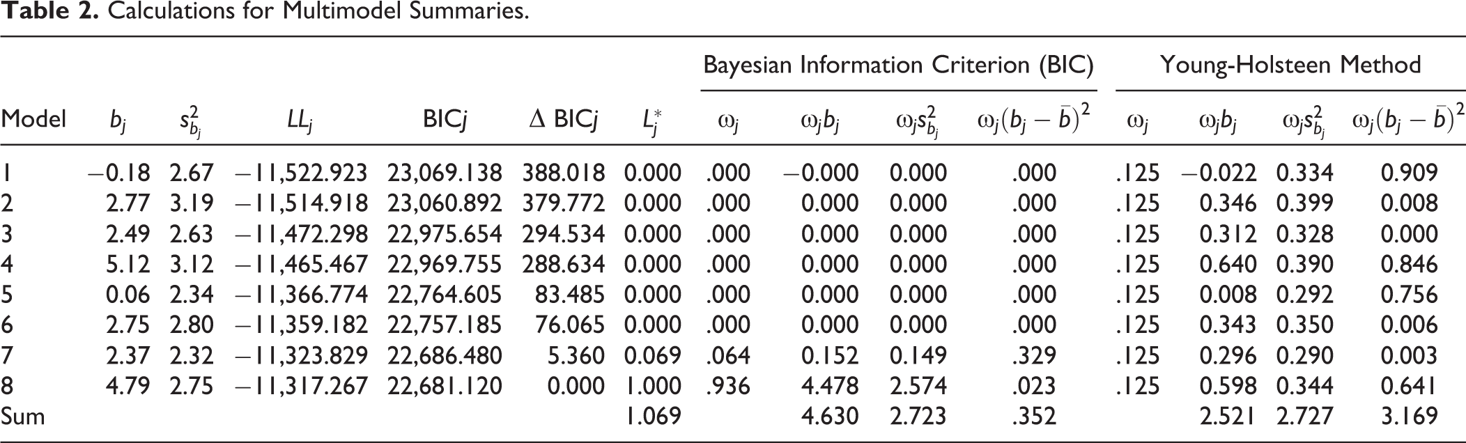
If we assign a uniform prior to the model space such that $τ_{j} = 1 / J$ , the model weights ω_j for the BIC method are given as follows:

ω_{j} = \frac{exp (- 0.5 \times Δ {BIC}_{j}) (1 / 8)}{\sum_{j} [exp (- 0.5 \times Δ {BIC}_{j}) (1 / 8)]}

= \frac{exp (- 0.5 \times Δ {BIC}_{j})}{\sum_{j} exp (- 0.5 \times Δ {BIC}_{j})} .

This definition follows naturally from equation (3), with the exact value of the model prior τ_j determined by the number of models under consideration. Yet as the above formulation suggests, the effect of the model prior τ_j on the model weight ω_j cancels out by the virtue of the fact that the value of τ_j happens to be constant across models. As it turns out, the YH method also begins with a uniform prior on the model space. The difference is that whereas traditional forms of model averaging allow priors to be revised in light of the data, the YH method commits to the equality assumption throughout. This is evident in the choice of model weights which, in this particular case, are defined as $ω_{j} = 1 / 8$ for the purposes of the YH portion of the analysis.

Using the above quantities, we compute estimates of $\bar{b} = \sum_{j} ω_{j} b_{j}$ , ${\bar{v}}_{s} = \sum_{j} ω_{j} s_{b_{j}}^{2}$ , and $v_{m} = \sum_{j} ω_{j} {(b_{j} - \bar{b})}^{2}$ . The differences between model averaging and the YH method are apparent. With nearly all of the weight—93.6 percent—placed on the full model, the estimated value of $\bar{b}$ using BIC-based model averaging—4.63—is, not surprisingly, nearly identical to the estimated effect of gender associated with the model in question. The same goes for the mean sampling variance ${\bar{v}}_{s}$ . The estimated modeling variance v_m using the BIC method—0.352—may seem low given how much the values of b_j tend to vary from one model to the next. As was the case with the other estimates, this is due to the fact that the bulk of the weight is concentrated on a single model. The variance that we do see is almost solely attributable to the difference in effect size between models 7 and 8, keeping in mind that the estimated modeling variance is still considerably less than the variance in observed effect size between the two models.

The results produced using the YH method are noticeably different, especially when looking that the mean point estimate $\bar{b}$ and the modeling variance v_m . The mean point estimate under the YH method is just 2.521, well below what was produced using the BIC method, where the mean point estimate was pulled toward the full model—the second most extreme model in the set. Conversely, the modeling variance produced using the YH procedure is roughly nine times higher than what it was under the BIC method! So while the BIC-based method suggests that we can be fairly confident in the full model as it stands, the YH method suggests that we should proceed with great caution when interpreting the results. Interestingly enough, the mean estimated sampling variance is roughly the same under both methods. This is a result of the fact that while the point estimates tend to vary a lot from one model to the next, the standard errors tend to remain fairly stable. Although this may not be the case in all scenarios, we will continue to see evidence of this trend in the examples considered below. As such, we will focus primarily on the modeling variance. Insofar as the values of b_j are the same regardless of whether we use model averaging or the YH procedure, variation in the estimated modeling variance is due entirely to differences in the model weights.

Numerical Variation Versus Statistical Uncertainty

The basic intuition behind both model averaging and the YH procedure is that numerical variation in a given parameter estimate is indicative of statistical uncertainty. This relationship is formally captured by the formula for modeling variance $v_{m} = \sum_{j} ω_{j} {(b_{j} - \bar{b})}^{2}$ . Using this formula, our goal is to quantify the degree of uncertainty associated with a given set of estimates. Taking the estimates in front of us as given, the estimated level of statistical uncertainty due to modeling variance is determined by the pairing of estimates and weights, with the distribution of model weights ω_j governing the conversion from variation to uncertainty. In the above example, we saw that the modeling variance was significantly lower when the weights were concentrated on a single model. Without making any assumptions about how weights should be assigned, we can get a sense of the mechanics underlying the production of statistical uncertainty by seeing how the estimated modeling variance v_m changes as weights w_j become increasingly concentrated.

Toward this end, I use simulation to construct hypothetical pairings of estimates and weights. Assuming a preferred model with one independent variable and 10 controls, each pass of the simulation begins by generating 2¹⁰ = 1, 024 coefficients b_j. The simulated coefficients are constructed by drawing a set of J = 1,024 values from a standard normal distribution and then rescaling the resulting values to ensure that the degree of numerical variation is constant from one run to the next. The degree of numerical variation is, by definition, equal to the unweighted modeling variance given by $\sum_{j} {(b_{j} - \bar{b})}^{2} / J$ , with $\bar{b} = \sum_{j} b_{j} / J$ . We can get a sense of the effect of weighting by comparing the unweighted modeling variance, which is fixed by design, to the estimated modeling variance produced under alternative weighting schemes. Weights were drawn at random from a Pareto distribution. While the scale parameter of the distribution was fixed at one, the shape parameter was systematically varied to produce variation in the degree of concentration, with lower parameter values tending to produce more concentrated weights. The resulting values were sorted to ensure that the rank order of coefficients with respect to weights was preserved across schemes.

Using the above method, I generated 10,000 sets of coefficients, along with 10 sets of weights for each. For any given combination of coefficients and weights, the effect of weighting can be measured in terms of the ratio of the weighted modeling variance to the unweighted modeling variance produced using the weights in question. Insofar as the distinction between the weighted and unweighted modeling variance corresponds to a distinction between statistical uncertainty and numerical variation, respectively, the ratio in question can be said to capture the rate at which numerical variation is converted into statistical uncertainty. A conversion rate of less than 1 indicates that the degree of statistical uncertainty is less than the degree of numerical variation. This exercise is admittedly artificial, in the sense that both the estimates and the weights exist independently of a given set of data. This setup is useful in two respects. First, it allows me to directly manipulate the level of concentration. Second, it allows me to remain completely agnostic about the origin of the weights. In this context, calculating statistical uncertainty is a purely mathematical operation, carried out without regard for principles of inference. The purpose is simply to describe what happens to our calculations as we begin to assign higher weights to a smaller number of models.

The results of the analysis are shown in Figure 1, which depicts variation in the central 50 percent of the distribution of conversion rates across weighting schemes. For ease of interpretation, weighting schemes are depicted in terms of the average concentration of weights associated with the underlying scale parameter as measured by the average Herfindahl–Hirschman index (HHI), which can range anywhere between 1/J and 1. The first thing to note is that there are conditions under which weighted modeling variance exceeds the unweighted modeling variance, as evidenced by the fact the upper bound of the central 50 percent of the distribution of conversion rates is clearly above 1 in many of the weighting schemes considered here. At the same time, the estimated modeling variance was more likely than not to be higher in the unweighted condition, even at the lowest levels of concentration. The conversion rate tends to be negatively associated with the degree of concentration, which makes this outcome even more likely as the degree of concentration increases.

Figure 1.

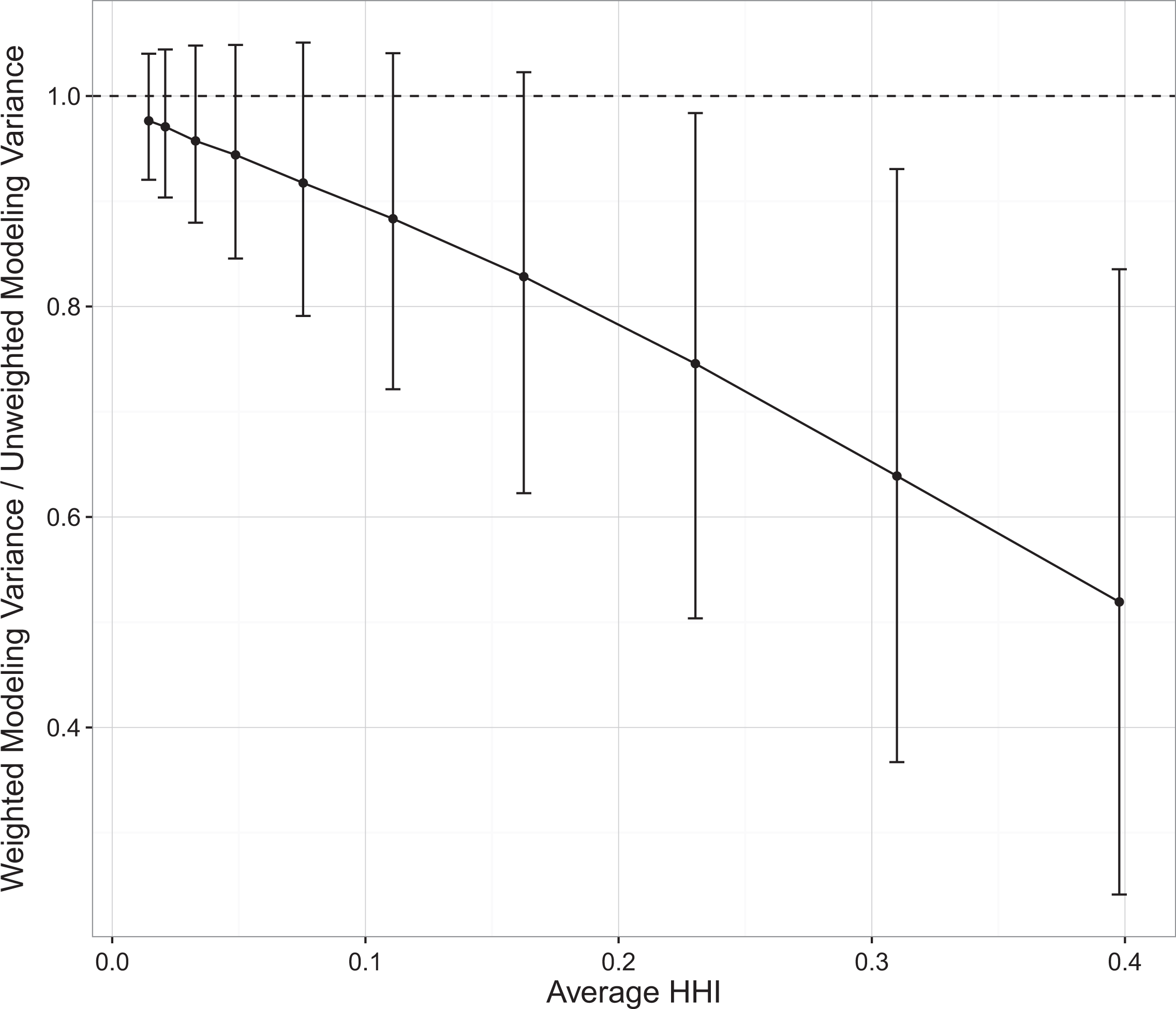
Distribution of conversion rates by concentration.

We find that the magnitude of the divergence between numerical variation and their weighted counterparts can be quite large. Considering only the middle 50 percent of estimates, we find cases where the weighted modeling variance (i.e., statistical uncertainty) is two, three, and even four times lower than the unweighted modeling variance (i.e., numerical variation). As one can imagine, the effects of weighting appear even more extreme once we consider the full range of the distribution.² In general, the results shown here not only indicate the conditions under which model averaging and the YH method are likely to produce different results but provide us with a sense of the nature of the differences in question. Insofar as traditional forms of model averaging assign weights on the basis of fit, the results of model averaging will typically differ from the results of the YH procedure when there are some models that fit better than others. Under these conditions, estimates of statistical uncertainty produced using the YH method will tend to be higher than those produced using traditional forms of model averaging. Given that few models are truly equal, we should expect to observe this type of divergence in most real-world scenarios. The question is not so much about whether model averaging and the YH method will produce different estimates of modeling variance; rather, the question is how much larger the variance will be under the YH method as compared to traditional forms of model averaging.

Examples

Using the data provided by YH as part of their mrobust package, I reran the analysis from the first two examples in YH, the first of which examines the relationship between wages and union membership and the second of which examines the relationship between mortgage approval and gender. In addition, I conducted a similar exercise using YH’s data on interstate migration. The resulting analysis is much simpler than that of YH, who use the migration example to show how their method can be used to simultaneously address questions regarding robustness with respect to the choice of controls, the choice of functional form, and the choice of data. For the purposes of the current discussion, I focus exclusively on the uncertainty resulting from the choice of controls. Toward this end, I use linear regression to model the relationship between the log of the number of interstate migrants and the difference in the income tax rate between the destination and the origin, with estimates of the number of interstate migrants come from the Internal Revenue Service. Following YH’s example, controls for the population size of both origin and destination are included in every model. Unlike YH, I did not adjust the standard errors.³

In each case, I compared the results produced using the YH method to the results produced using a range of model averaging procedures, including Akaike information criterion (AIC)-based averaging, approximate Bayesian averaging using the BIC, and fully Bayesian model averaging using both a Zellner–Siow prior, as well as a hyper-g prior (a = 3) . Note that in the case of the latter two procedures, the priors in question refer to the priors on the parameters not the model space. Details of these procedures are provided by Montgomery and Nyhan (2010). In the context of model averaging, it is fairly standard to average over all possible models. For the sake of comparability, however, I follow YH and focus exclusively on models containing the parameters of interest, thus bracketing out the question of whether these variables should be included in the first place. I also follow the example of YH in assigning a uniform prior to the model space. Calculations were carried out using the bas.lm routine included as part of the BAS package in R (Clyde 2016).⁴

The results of the analysis are summarized in the Figure 2, which depicts the decomposition of variance by prior. The results are quite striking. In all three cases, the estimated modeling variance under the YH procedure tends to exceed that of other methods. This trend is especially pronounced in the union membership and gender examples, where the modeling variance—which is more or less nonexistent when using standard forms of model averaging—virtually doubles the size of the total variance! The discrepancy is less sizable in the case of tax advantage, the only example of the three in which the mean estimated sampling variance appears to exceed the modeling variance. Our expectation is that the degree of discrepancy between results produced using the YH method and results produced using standard forms of model averaging should roughly correspond to the extent to which the weights used for model averaging tend to concentrate on a single model.

Figure 2.

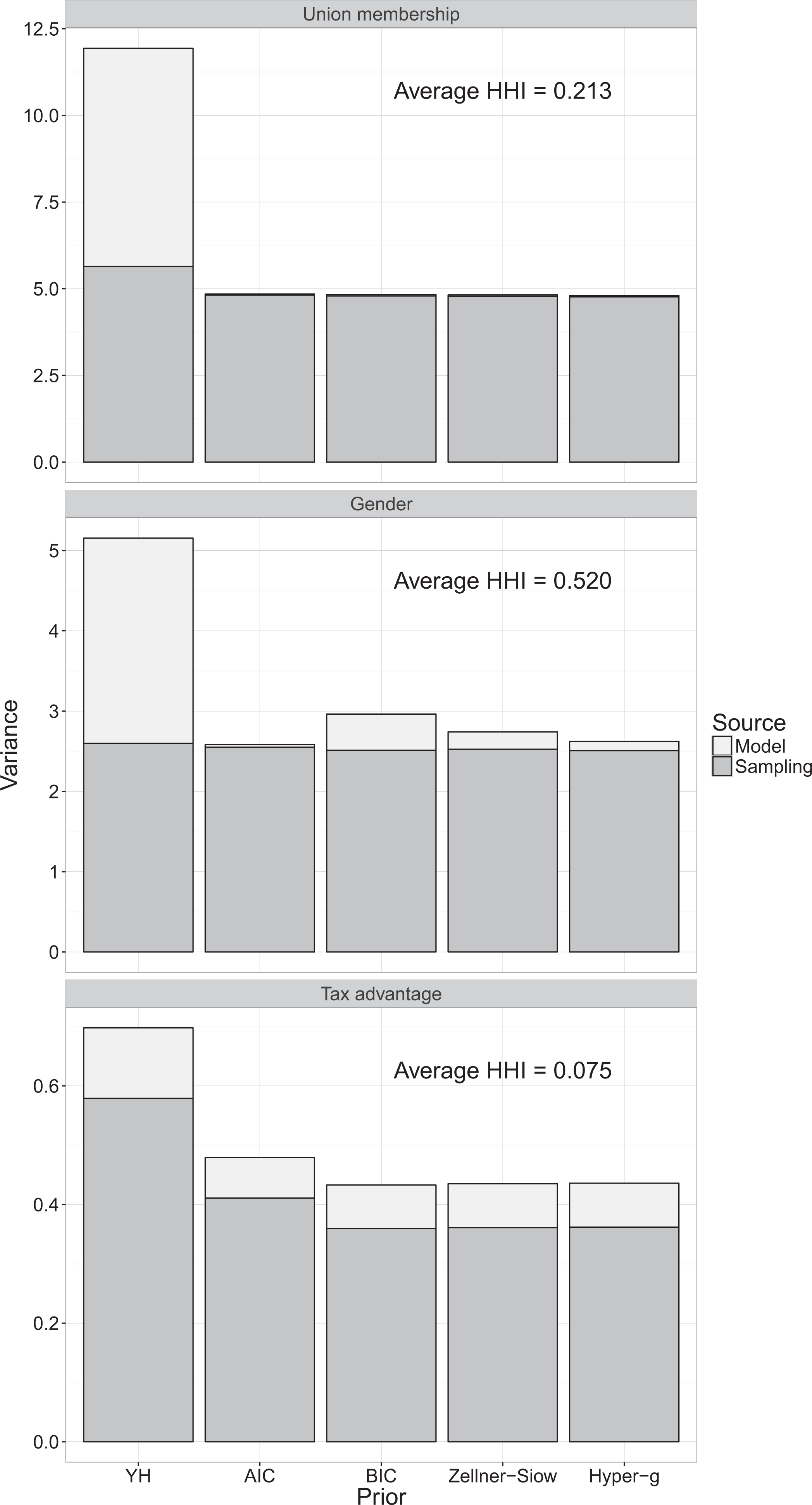
Decomposition of variance by prior.

To measure the degree of concentration, I calculated the average HHI value associated with the distribution of weights resulting from each of the model averaging procedures. I then took the average for each example. As we might expect, the distribution of estimated model weights in the tax advantage example is less concentrated than the other two. At the same time, we see that the relationship between discrepancy and concentration is less than perfect, as evidenced by the comparison between the union wage and gender examples, which produce comparable levels of discrepancy in spite of the fact that the estimated level of concentration in the gender example is almost 2.5 times higher than that in the union wage example. This is consistent with the results of the simulation, which showed that while the divide between weighted and unweighted estimates clearly increases along with the level of concentration, there is a considerable amount of variation around this trend. The key point here is that the potential for discrepancy between the YH procedure and standard forms of model averaging is apparent in real-world examples, with the YH procedure producing a higher estimated modeling variance than conventional forms of model averaging, as we would tend expect given the results of the simulation. The question is whether this increased uncertainty is warranted.

Why Weight?

Up to this point, we have focused exclusively on the effects of weighting, setting aside the question of why one would weight in the first place. The simple answer is that weighting is what gives us inferential traction. This line of argument is not tied to any particular philosophy—it follows naturally from basic probability theory. When working with a single model, inferences are based on a distribution whose properties are, in effect, conditional on the choice of model in question. This is true regardless of whether we think about inference in terms of the sampling distribution of the estimate or the posterior distribution of the parameter. Multimodel inference addresses the problem of model dependence by combining these conditional results to generate a statement about the unconditional distribution of a given quantity of interest.

To help fix ideas, we can start with an analogy to a one-way analysis of variance (ANOVA) in which in the unconditional distribution of some random variable Y can be understood as a mixture of conditional distributions, each of which is associated with a particular group of observations. Here we are concerned not so much with ANOVA as a formal test but as a way of thinking about the world. From this perspective, the question is, how much does each of the conditional distributions contribute to the unconditional distribution? If we think about any standard ANOVA problem, it should be fairly intuitive that groups do not necessarily contribute equally. We find instead that a group’s contribution is proportional to its share of the population, which is the same thing as saying that a group’s contribution is proportional to the probability of selecting a member of that group at random.

If group membership is represented by a discrete random variable X, then the law of total probability says that the unconditional distribution of the outcome Y can be expressed as follows:

p (Y) = \sum_{j} p (Y | X = j) p (X = j),

where $p (Y | X = j)$ refers to the conditional distribution of Y associated with group j, while p(X = j) refers to the marginal probability of selecting a member from group j. For the purpose of this discussion, we are unconcerned with whether the conditional distribution $p (Y | X = j)$ meets the standard ANOVA assumptions. All we care about here is the idea that the unconditional distribution of a random variable can be recovered from a set of conditional distributions, provided that these distributions are weighted by the probability that the condition in question holds. Replacing groups with models, this basic approach extends naturally to the case of multimodel inference, with the exact nature of the underlying distributions depending on one’s choice of statistical philosophy.

Applying the law of total probability to the problem of Bayesian regression, Leamer (1978:117-18) famously proposed that

p (β | D) = \sum_{j} p (β | M_{j}, D) p (M_{j} | D),

where D refers to a given set of data, M_j refers to model j, $p (β | D)$ refers to the posterior distribution of β, $p (β_{j} | M_{j}, D)$ refers to the posterior distribution of β_j (i.e., the posterior distribution of β associated with M_j), and $p (M_{j} | D)$ refers to the posterior probability of M_j. The posterior distribution $p (β | D)$ is, in effect, a weighted combination or mixture of the set of conditional distributions given by $p (β | M_{j}, D)$ , with the posterior model probabilities $p (M_{j} | D)$ serving as weights. The standard model averaging equations (i.e., equations [1] and [2]) arise out of an effort to estimate the expectation and variance of the resulting distribution. While the quantities being estimated here are decidedly Bayesian in origin, we can derive similar results using classical sampling theory as well (see Burnham and Anderson 2002:153-64). So regardless of which particular philosophy one happens to adopt, there seems to be a general consensus around the idea that, from a theoretical perspective, weighting is appropriate, if not required.

The practical difficulty lies in the fact that in order to weight our estimates, we need to be able to calculate the probability of the models from which they were drawn. For the moment, we will focus exclusively on the Bayesian case, where the probability in question can be ambiguously interpreted in terms of the posterior model probability $p (M_{j} | D)$ defined below:

p (M_{j} | D) = \frac{p (D | M_{j}) p (M_{j})}{\sum_{j} p (D | M_{j}) p (M_{j})},

where $p (D | M_{j})$ refers to the marginal likelihood of the data under model j and p(M_j) refers to the prior probability of the model in question. By multiplying the model prior by the marginal likelihood of the data under the model in question, we are in effect updating our priors on the basis of the observed data. While priors are specified directly by the researcher, the marginal likelihood needs to be calculated. Depending on the nature of the problem, we may be able to calculate the marginal likelihood directly. In other cases, we are forced to rely on approximation, with the Laplace method in particular emerging as a popular choice.

This approach can be used to motivate the derivation of the BIC, which, under certain conditions, is roughly proportional to the log marginal likelihood (see Raftery 1995:145). If we assume that all models are equally likely a priori, the posterior model probability of any given model can then be calculated as follows:

p (M_{j} | D) \approx \frac{exp (- 0.5 \times {BIC}_{j})}{\sum_{j} exp (- 0.5 \times {BIC}_{j})},

with the latter quantity serving as the model weight ω_j, as per the example from which we began. Starting with the law of total probability, we can now see very clearly how and why models come to be weighted by fit, whether that be understood in terms of the marginal likelihood itself or some approximation thereof. Non-Bayesian approaches to the problem proceed in a similar fashion. Burnham and Anderson (2002:74-77), for example, propose using variants of the AIC in place of the (approximate) marginal likelihood. While the resulting weights can technically be recast as posterior model probabilities, they are more directly interpretable as estimates of the probability that a given model is the Kullback–Leibler best model in the set.

Endogeneity and Other Misguided Fears

According to YH, standard forms of model averaging weight estimates in one of the two ways—by model fit or by Bayesian prior. They balk at the practice of weighting by fit on the grounds that measures of fit are only valid under the assumption of exogeneity. It is hard to know what to do with this claim. Measures of fit—marginal likelihood and approximations thereof being among the most important—are meaningfully defined without regard to the quality of the predictors. So while there may be conditions under which the inclusion of an endogenous predictor causes a better fitting model to produce worse estimates than would otherwise be the case, it is not as if there is a systematic relationship whereby measures of fit are necessarily subject to upward bias in the presence of endogenous predictors. This is not to suggest that the question of endogeneity is somehow irrelevant. The point is that to the extent that the assumption of exogeneity is a problem, we need to be clear about the fact that the assumption in question applies to the model itself and thus holds regardless of whether we chose to weight the resulting estimates by fit.

The idea of using unweighted estimates to address concerns regarding endogeneity was first proposed by Sala-i Martin (1997). Introduced in the context of work on economic growth where the threat of endogeneity due to reverse causation—which might lead to a spuriously high fit—happens to loom especially large (see Brock and Durlauf 2001:237-38), the use of unweighted estimates does not appear as a refutation of standard forms of model averaging but as an ad hoc check designed to deal with the specific empirical problem at hand. Indeed, not only did Sala-i Martin continue to contribute to the development of standard model averaging procedures (see Sala-i Martin, Doppelhofer, and Miller 2004), he would also go on to suggest in passing that model averaging might be the solution to the endogeneity problem (see Sala-i Martin 2001:281). This suggestion has been borne out by a growing body of work showing that standard approaches to modeling endogenous regressors extend naturally to the case of model averaging (e.g., Durlauf, Kourtellos, and Tan 2008; Karl and Lenkoski 2012; Koop, Leon-Gonzalez, and Strachan 2012; Lenkoski, Eicher, and Raftery 2014), thus alleviating any lingering concerns as to whether an otherwise remediable problem is somehow damning in a multimodel setting.

This is all to say that endogeneity is neither inherently at odds with the prospect of model averaging nor is the use of unweighted estimates an unambiguous solution. Insofar as the inclusion of endogenous predictors leads to biased estimates, the problem with endogeneity in the context of multimodel inference is that we might overweight bad estimates, an outcome that seems just as likely when we assign the same weight to each model. Certainly, some of our models are better than others, however that may be defined. Again, whatever problems there are with a model, these adhere at the level of the model itself and need to be handled accordingly. Endogeneity and causality in particular have been highlighted as areas that are not in and of themselves addressed through standard forms of model averaging (Montgomery and Nyhan 2010:266). Model averaging can, however, be used to improve existing solutions to the problems in question as noted above with respect to the issue of endogeneity. We have seen similar progress in the area of causality and counterfactual inference as evidenced by an emerging line of work that combines model averaging with propensity score matching (e.g., Kaplan and Chen 2012; Zigler and Dominici 2014).

In terms of the question of Bayesian priors, YH contend that weighting models on the basis of one’s priors privileges model assumptions emanating from the private beliefs of the researcher, thus giving rise to an asymmetry of information between audience and analyst. This line of critique is largely out of step with how priors work in practice. In the first place, it is common to report one’s priors, so while these may begin as private beliefs, they are eventually made public. In this sense, Bayesian methods tend to be fairly transparent. More importantly, when it comes to assigning weights, priors do not exist independently of fit as YH seem to let on. As shown in equation (8), the assignment of weights is consonant with a process of Bayesian updating in which prior assumptions are revised in light of the data as captured by some measure of fit. In this setting, failure to account for fit is tantamount to a refusal to learn from the data.

This is where the YH procedure really diverges from conventional forms of model averaging. It is not uncommon to begin—as YH do—from the assumption that all models are equally likely. In most cases, however, prior equality quickly gives way to posterior distinction. Once we look at the results, we usually have a pretty good sense of which models seem to work and update our priors accordingly. In the context of the YH procedure, on the other hand, the assumption of equality effectively supersedes the traditional distinction between prior beliefs and posterior estimates. The irony is that in attempting to avoid the assumptions that come with standard forms of model averaging, the YH method makes a stronger and even less plausible assumption of its own. To paraphrase a reviewer, the YH method is, in effect, a degenerate form of Bayesian model averaging in which we never update our priors. From a technical perspective, this is unambiguously true, in the sense that one can replicate the results of YH’s mrobust command using existing model averaging routines by simply replacing the posterior weights with their corresponding priors.

Coverage, Bias, and Out-of-Sample Prediction

The argument above suggests three things. First, the relationship between numerical variation and statistical uncertainty is systematically affected by the extent to which the assigned weights are concentrated in a single model, with the conversion rate tending to decline as concentration increases. Second, the propensity for divergence has practical implications insofar as the YH method and conventional forms of model averaging tend to produce different results in real-world applications. Third, to the extent that they approximate the probability of a given model, weights are integral to the process of estimation and inference. We thus have every to think not only that we should weight, but that the decision to weight is likely to have a very real bearing on the quality of the results. To illustrate this point, I turn to simulation. The advantage of using simulation is that we know the value of the underlying parameters ahead of time, thus allowing us to quantify the extent to which any given procedure captures the characteristics of the data generating process.

To put it another way, simulation helps us to evaluate a method’s inferential capacity, by which I mean the capacity of a method to translate descriptive statements about the data in front of us into claims about the larger population from which those data were drawn. The role of inference in the YH method is, however, somewhat ambiguous. Motivated in large part by the threat of false positives, the tools proposed by YH are designed to assess the extent to which one’s preferred estimate depends on a particular model or assumption set. So while allowing for the prospect of inference at the level of the individual model, YH ultimately stop short of multimodel inference. At the same time, the inferential properties of a measure such as the robustness ratio can easily be evaluated using standard methods. More specifically, if we recast the robustness ratio in terms of a confidence interval, we can objectively asses its inferential performance in terms of coverage probability or the percentage of trials in which the interval captures the true value of the parameter of interest.

The analysis below focuses in particular on the relationship between the independent variable x and the outcome y associated with the model:

y = α + β x + Γ_{1} z_{1} + Γ_{2} z_{2} + θ_{1} w_{2} + θ_{2} w_{3} + θ_{3} w_{3} + ε,

where α refers to the intercept, β refers to the coefficient of interest, and ε refers to a random disturbance. We assume that α = 0, β = 1, and $ε \sim N (0, σ^{2})$ , with the residual standard error σ set to 2.5 throughout. The remaining variables $z = [z_{1} z_{2}]$ and $w = [w_{1} w_{2} w_{3}]$ serve as controls. The distinction between z and w lies in the nature of their relationship to the outcome y, as reflected in the differences between their corresponding parameter vectors Γ = 1 and θ = 0. While the variables making up w are ultimately irrelevant to the data generating process, they are included in the formulation above in order to highlight their role in the construction of the model space.

The vector of predictors $x^{*} = [x w z]$ is drawn from a multivariate normal distribution with a 1 × K mean vector of 0 and a variance–covariance of $Σ_{x^{*}}$ , where $Σ_{x^{*}}$ refers to a K × K variance–covariance matrix, with K = 6 as implied by the formula above. The diagonal entries of $Σ_{x^{*}}$ are set to one. When coupled with a mean vector of 0, this is equivalent to assuming a model with six covariates, each of which is normally distributed such that $x_{k}^{*} \sim N (0, 1)$ for any given predictor k. The off-diagonal entries of $Σ_{x^{*}}$ were systematically manipulated to produce variation in the distribution of estimates. More specifically, I varied the pairwise correlation between x and the members of z, while setting the remaining off-diagonal elements to 0. I consider four scenarios in particular. In case 1, I assume that x and z are independent. In case 2, I relax the assumption of independence by introducing a moderate pairwise correlation between x and the members of z, with ρ = 0.3 for both z₁ and z₂. In case 3, I assume a strong pairwise correlation between x and the members of z, with ρ = 0.6 for both z₁ and z₂. In case 4, I again allow for moderate correlation between x and z, though in this instance I assume that ρ = 0.3 for z₁ and ρ = −0.3 for z₂, such that models omitting z in its entirety tend to produce more accurate estimates than models in which either z₁ or z₂ is included on its own.

For each case, I generated 10,000 samples of size N = 1,000. Using these data, I assess the relative performance of the YH procedure in terms of not only coverage but bias and out-of-sample prediction as well. The discussion of bias follows naturally from the discussion of coverage, in that bias in the point estimate inevitably carries over to the resulting interval. Together, measures of coverage and bias are used to quantify the ability of the YH procedure to speak to the parameter of interest β. Moving beyond the traditional YH framework, I also consider the effect of weighting on out-of-sample prediction. Although not especially common in sociology, out-of-sample performance is a standard metric in fields such as machine learning, where ensemble methods—including model averaging—are commonly used for the purpose of prediction. Lack of familiarity aside, out-of-sample performance is an intuitive measure of a method’s ability to capture the basic properties of the data generating process.

Results

The results of this exercise are shown in Table 3. I consider two types of intervals, the first of which is the traditional model-specific interval given by $b_{j} \pm 2 \times s_{b_{j}}$ , where $s_{b_{j}}$ refers to the standard error of b_j as given before. Estimates of b_j and $s_{b_{j}}$ were derived using both the true model $y = α + β x + Γ^{'} z + ε$ and the full model $y = α + β x + Γ^{'} z + θ' w + ε$ . The second type of interval is the model-averaged interval given by $\bar{b} \pm 2 \times \sqrt{v_{t}}$ . While this particular form of interval is known to be distributionally problematic (see Hjort and Claeskens 2003), its construction parallels the robustness ratio actually calculated by YH in their examples.⁵ Estimates of $\bar{b}$ and v_t were derived using both the YH method and the various model averaging procedures considered above. The estimates for any given sample are based on the J = 32 possible models containing the variable of interest. The model weights ω_j are set to 1/J when using the YH method but are otherwise freely estimated.

Table 3.

Coverage, Bias, and Predicton Error by Method.

Case	Interval	$\bar{PE}$	$\bar{MESV}$	$\bar{MV}$	CP	$\bar{LB}$	$\bar{UB}$	$\bar{W}$	B	$\bar{MSPE}$
1	True model	1.00	.006	.000	0.955	.841	1.157	0.317	−.001	6.282
1	Full model	1.00	.006	.000	0.955	.841	1.158	0.317	−.001	6.300
1	YH	1.00	.007	.001	0.966	.823	1.176	0.353	−.001	6.304
1	AIC	1.00	.006	.000	0.955	.841	1.158	0.317	−.001	6.300
1	BIC	1.00	.006	.000	0.955	.841	1.158	0.317	−.001	6.300
1	Zellner-Siow	1.00	.006	.000	0.955	.838	1.154	0.316	−.004	6.300
1	Hyper g	0.99	.006	.000	0.954	.832	1.148	0.315	−.010	6.300

2	True model	1.00	.008	.000	0.956	.825	1.175	0.350	−.000	6.282
2	Full model	1.00	.008	.000	0.955	.824	1.175	0.351	−.000	6.301
2	YH	1.31	.008	.046	0.950	.852	1.778	0.926	.315	6.484
2	AIC	1.00	.008	.000	0.956	.825	1.175	0.350	−.000	6.301
2	BIC	1.00	.008	.000	0.955	.825	1.175	0.350	−.000	6.301
2	Zellner-Siow	1.00	.008	.000	0.955	.823	1.172	0.350	−.003	6.301
2	Hyper g	0.99	.008	.000	0.954	.819	1.168	0.349	−.007	6.301

3	True model	1.00	.022	.000	0.953	.703	1.302	0.599	.003	6.289
3	Full model	1.00	.023	.000	0.953	.703	1.303	0.600	.003	6.308
3	YH	1.77	.013	.212	0.860	.828	2.713	1.885	.770	7.250
3	AIC	1.00	.022	.000	0.953	.703	1.302	0.599	.003	6.308
3	BIC	1.00	.022	.000	0.953	.703	1.302	0.599	.003	6.308
3	Zellner-Siow	1.00	.022	.000	0.954	.701	1.300	0.598	.000	6.308
3	Hyper g	1.00	.022	.000	0.954	.699	1.296	0.597	−.002	6.308

4	True model	1.00	.008	.000	0.953	.825	1.175	0.350	−.000	6.281
4	Full model	1.00	.008	.000	0.953	.825	1.175	0.351	−.000	6.300
4	YH	1.00	.008	.055	1.000	.499	1.501	1.002	−.000	6.350
4	AIC	1.00	.008	.000	0.952	.825	1.175	0.350	−.000	6.300
4	BIC	1.00	.008	.000	0.953	.825	1.175	0.350	−.000	6.300
4	Zellner-Siow	1.00	.008	.000	0.954	.822	1.172	0.350	−.003	6.300
4	Hyper g	0.99	.008	.000	0.953	.816	1.165	0.348	−.009	6.300

Note: $\bar{PE}$ = average point estimate; $\bar{MESV}$ = average mean estimated sampling variance; $\bar{MV}$ = average modeling variance; CP = coverage probability; $\bar{LB}$ = average lower bound; $\bar{UB}$ = average upper bound; $\bar{W}$ = average width; B = bias; $\bar{MSPE}$ = average mean squared prediction error.

For each combination of case and interval, I report the average point estimate $\bar{PE}$ along with the average mean estimated sampling variance $\bar{MESV}$ and the average modeling variance $\bar{MV}$ . The latter two quantities provide independent summaries of the quantities making up the total variance.⁶ As discussed above, the parameters of the data generating model were systematically manipulated to generate variation in the distribution of raw estimates associated with each case. The effects of the manipulation are apparent in the results for the YH interval. Looking at case 1, we see that when the predictors in the data generating model are independent, not only is the average YH point estimate equal to the true value β = 1 but the average modeling variance is nearly 0. Once we introduce collinearity, the YH point estimate has the potential to drift off depending on the nature of the correlation structure. As the results of case 4 suggest, the average unweighted point estimate can match the true value even in the presence of correlated predictors, though we continue to observe nonzero modeling variance as expected.

When it comes to assessing the inferential properties of the YH method, the primary point of reference is the coverage probability (CP) which, as per the discussion above, measures the proportion of trials in which the confidence interval associated with a given estimate captures the true parameter value. In an effort to depict the typical interval, I have included information on the average lower bound $\bar{LB}$ , the average upper bound $\bar{UB}$ , and the average width $\bar{W}$ . The underlying intervals assume a critical value of 2. This value was purposely chosen to coincide with YH’s rule of thumb for determining robustness. Using intervals of this width, we expect a nominal coverage rate of around 95.5 percent. We find that when the data are generated using orthogonal predictors as in case 1, a YH interval captures the true effect β in 96.6 percent of samples. This is a bit higher than what we might expect, but it is neither unreasonable nor is it radically out of step with what we observe using either model-specific intervals or standard forms of model averaging, all of which produce coverage probabilities in the same neighborhood as the nominal rate. Yet unlike what we see with either the model-specific intervals or their model-averaged counterparts, the coverage probability associated with the YH interval is sensitive to the nature of the underlying correlation structure.

Looking across the four cases, we find that the coverage probability associated with the non-YH intervals holds steady between 0.952 and 0.956. In contrast, coverage under the YH method ranges from anywhere between 0.86 and 1, meaning that the resulting coverage probabilities can be either well above or well below the nominal rate depending on the nature of data generating process. To understand how this plays out, we need to consider the behavior of the estimated variance as well as the corresponding point estimate. As we move away from the case of orthogonal predictors where the expected modeling variance is equal to 0 by definition, the width of the YH interval increases accordingly. Comparing the average width of the interval produced using the full model to the average width of the interval produced using the YH method, we find that the typical YH interval is 1.11 times larger in case 1, 2.64 times larger in case 2, 3.14 times larger in case 3, and 2.86 times larger in case 4.⁷ In other words, the results suggest that the use of the YH interval in this context entails doubling and tripling the width of intervals that already reproduce the nominal coverage rate. The variation in excess width across cases corresponds with variation in the average modeling variance, as we would expect.⁸

Whether the coverage rate under the YH interval falls above or below the nominal rate depends on the extent to which the unweighted average of model-specific estimates deviates from the true parameter value. Much like the inflation of the standard error, the degree of bias in the YH point estimate depends on the underlying correlation structure. Unlike the width of the interval, however, the deviation between the point estimate and the true parameter value does not necessarily correspond with the expected value of the unweighted modeling variance. This can be seen by examining changes in the observed bias B representing the difference between the average estimate across samples and the true value of the parameter being estimated. Looking at the results for the YH method, we see the degree of bias increase as we move away from orthogonal predictors in case 1, toward moderate correlation in case 2, and strong correlation in case 3.

In these cases, the propensity for an upward bias in coverage due to the use of inflated standard errors is tempered by the bias in their respective point estimates, resulting in subnominal coverage rates. This is what we would usually expect from a biased estimator. The issue in this case is that in order to produce a downward bias in coverage, the bias in the point estimate needs to be severe enough to counter the inflation in the standard error. Note that a correlation between x and the members of z does not guarantee a biased point estimate. This can be seen in case 4, where the various incarnations of omitted variable bias happen to offset one another such that the unweighted average of b_j equals the true effect β. In this instance, the interval behaves exactly as we would expect given the degree of numerical variation in the underlying point estimates.

To this point, I have focused on inference with respect to a single parameter. I also consider overall performance as measured by the capacity for out-of-sample prediction. With this goal in mind, I simulated a second set of data for each trial using the same data generating process as before. For any given trial, the question is how well a model or ensemble based on the first set of data—the data that produced the results described above—predicts outcomes in a second set of data that were omitted from the estimation process. The correspondence between the observed and predicted values associated with a given sample can be measured in terms of the mean squared prediction error $MSPE = | | y - \hat{y} | |^{2}$ , where y refers to a vector of observed outcomes and $\hat{y}$ refers to a vector of predictions. When considering model-specific parameter estimates based on the true or full model, predicted values are constructed in the usual way. When considering the YH method or one of the more conventional model averaging procedures, we begin by calculating an average parameter estimate for each of the parameters in the full model. We can then use the resulting parameter vector as we would the parameter vector from the full model.⁹

When constructing average parameter estimates, I consider models both with and without the variable of interest x. The resulting model space is comprised of a total of J = 64 models. As before, the model weights ω_j are set to 1/J when using the YH method and freely estimated otherwise. When a variable is omitted from a model, the corresponding parameter estimate is assigned a value of 0. Allowing variables to be omitted in this manner causes the average parameter estimate to be shrunk accordingly. In the case of the YH method, the estimate is simply cut in half. In all other cases, the estimate is shrunk by a factor equal to the inverse of the sum of the weights associated with the models in which the variable is included. In this formulation, a variable is, in effect, only as good as the models in which it appears. The implication is that variables that are weak or uncertain have less of an influence on the predicted value than they would otherwise.

Table 3 reports the average MSPE value across samples. Not surprisingly, the true model outperforms its competitors in all four cases. We find that conventional model averaging procedures do as well, if not slightly better than the full model, with only modest variation in predictive performance across cases. The performance gain due to model averaging is admittedly slight, though that is to be expected, given how close the full model is to the true model. The performance of the YH method, however, deviates quite a bit from that of the other methods. As was true before, the results differ considerably across cases. In the presence of orthogonal predictors, the performance of the YH method is only slightly worse than that of the other procedures. Outside this case, however, the YH method predictions are noticeably worse than those of the other methods, with the exact degree of divergence depending on the specific correlation structure at hand.

Discussion

The results above are clear. In all four cases, the coverage probability for the YH interval deviates from that of its competitors, all of which—including conventional forms of model averaging—produce coverage rates around the nominal level. This deviation is a product of a case-specific interplay between the width of the interval and the accuracy of the point estimate. While the YH interval tended to be much wider than any of the alternatives considered here, this only translated into above-nominal coverage when coupled with an unbiased point estimate. In the presence of a biased point estimate, coverage could be either above or below the nominal rate depending on whether the degree of bias was enough to offset the size of the interval. There is no reason to think that any of the model-averaged point estimates—either weighted or unweighted—should necessarily approximate the true parameter value. In the simple cases above, however, we only observe sizable bias when looking at the unweighted estimates associated with the YH method.

It might be argued that when it comes to the YH method, what you lose in precision and accuracy, you make up for in flexibility and ease of use. Insofar as any methodological choice is subject to scrutiny within the YH framework, there are almost certainly scenarios covered by YH that do not fall under the umbrella of standard forms of model averaging.¹⁰ As the discussion above makes clear, the inferential cost of using unweighted estimates is far from trivial, especially when there is a discernible difference in the quality of the underlying models. Fortunately, the bulk of the tools introduced by YH already have some direct alternative in the model averaging literature. Readers are directed to the work cited in Table 4, which provides a list of relevant citations related to carrying out YH-style analysis using existing tools, focusing in particular on techniques that extend beyond traditional forms of variable selection. I have included a list of relevant R packages where applicable. Versions of these programs have been available since at least 2012, with the oldest of the three—BMA (Raftery et al. 2015)—first appearing in 2005. A quick search suggests that the earliest incarnations of what became BMA have been available as an S routine since 1995, if not earlier.

Table 4.

Key Features of the Young-Holsteen Method and Their Model Averaging Analogs.

Feature	Analog	References	R Package
Modeling distribution	Posterior distribution	Bartels (1997)	BayesVarSel (Garcia-Donato and Forte 2016)
		Kass and Raftery (1995)
		Montgomery and Nyhan (2010)
		Montgomery and Nyhan (2010)	BAS (Clyde 2016)
		Raftery, Madigan, and Hoeting (1997)	BMA (Raftery et al. 2015)
		Western (1996)	BMS (Zeugner and Feldkircher 2015)
			BMS (Zeugner and Feldkircher 2015)
Functional form robustness	Distributional uncertainty	Burnham and Anderson (2002)
		Carlin and Polson (1991)
		Kass and Raftery (1995)
		Raftery (1996)
		Western (1996)
	Link uncertainty	Burnham and Anderson (2002)
		Czado and Raftery (2006)
		Draper (1995)
		Kass and Raftery (1995)
		Raftery (1996)
	Outcome transformation	Burnham and Anderson (2002)
	Predictor definition	Montgomery and Nyhan (2010)	MuMIn (Barton 2016)
Influence	Jointness	Crespo Cuaresma et al. (2015)	BayesVarSel (Garcia-Donato and Forte 2016)
Influence	Jointness	Doppelhofer and Weeks (2009)	BayesVarSel (Garcia-Donato and Forte 2016)

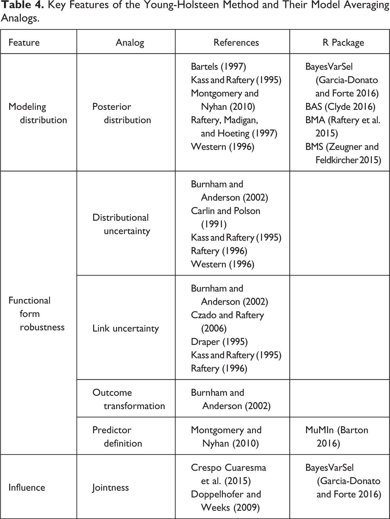
A full discussion of the intricacies of these various methods is well beyond the scope of this article.¹¹ For the purposes of the present discussion, the key point is that, contrary to YH’s claim, conventional forms of model averaging are by no means uniquely concerned with the choice of variables. Indeed, discussions regarding the distribution of estimates as well as uncertainty in the choice of family and link are evident in seminal papers such as that of Kass and Raftery (1995) who, along with Raftery (1995), helped to popularize the use of the BIC in the mid-1990s.¹² Since then, we have seen work touching on topics such as the transformation of outcomes (Burnham and Anderson 2002), the definition of predictors (Montgomery and Nyhan 2010), and the extent to which predictors work in combination with one another (Crespo Cuaresma et al. 2015; Doppelhofer and Weeks 2009). When it comes to implementation, however, the primary focus is still on variable selection. Yet, this is as true of the mrobust package provided by YH as it as of most other model averaging routines. To replicate YH’s work on functional form robustness, for example, one has to combine estimates across multiple rounds of variable selection and then summarize the results in the usual way. The main point of difference among available packages lies in the choice of priors, with minor differences in the availability of convenience functions related to tasks such as the construction of posterior plots (Clyde 2016; Garcia-Donato and Forte 2016; Raftery et al. 2015; Zeugner and Feldkircher 2015), the construction of jointness statistics (Garcia-Donato and Forte 2016), and the omission of models from the model space (Barton 2016).

In the spirit of full disclosure, it is worth noting that I provided comments on an earlier version of YH’s paper, though the comments I offered then looked quite a bit different than the comments offered here. At the time, I was not fully aware of the possibility of model averaging, though I realize in retrospect that the concept appeared in Young’s earlier work (see Young 2009:382-83). I remain confident that the methods proposed by YH can help us make sense of general patterns in the data in front of us. My concern, simply stated, is that these patterns do not necessarily translate into meaningful statements about the underlying quantities of interest. The benchmarks proposed by YH assume a probabilistic framework that no longer applies once we insist on the equality of models. While I have a hard time recommending YH’s method as an inferential procedure, the motivating principle is absolutely correct and I remain inspired by their commitment to improving methodological practice. Regardless of whether we think about the issue in terms of robustness or inference, model uncertainty is a real concern that applies to the vast majority of quantitative research in sociology. We are well-served by following YH’s lead in trying to find tools to help us address this problem.

Footnotes

Acknowledgment

Thanks are due to John Levi Martin and three anonymous reviewers for forcing me to clarify the argument. I would also like to acknowledge Jon Kropko for encouraging me to write this in the first place. Andrew Hayashi provided helpful comments along the way.

Declaration of Conflicting Interests

The author(s) declared no potential conflicts of interest with respect to the research, authorship, and/or publication of this article.

Funding

The author(s) received no financial support for the research, authorship, and/or publication of this article.

Notes

References

Bartels

Larry M.

1997. “Specification Uncertainty and Model Averaging.” American Journal of Political Science 41:641–74.

Barton

Kamil

. 2016. “MuMIn: Multi-model Inference.” R package version 1.15.6. (https://CRAN.R-project.org/package=MuMIn).

Brock

William A.

Durlauf

Steven N.

. 2001. “What Have We Learned from a Decade of Empirical Research on Growth? Growth Empirics and Reality.” The World Bank Economic Review 15:229–72.

Burnham

Kenneth P.

Anderson

David R.

. 2002. Model Selection and Multimodel Inference: A Practical Information-theoretic Approach. 2nd ed. New York: Springer.

Carlin

Bradley P.

Polson

Nicholas G.

. 1991. “Inference for Nonconjugate Bayesian Models Using the Gibbs Sampler.” The Canadian Journal of Statistics 19:399–405.

Clyde

Merlise A.

2016. “BAS: Bayesian Adaptive Sampling for Bayesian Model Averaging.” R package version 1.3.0. (https://CRAN.R-project.org/package=BAS).

Cuaresma

Crespo

Jesus

Bettina Grun

Hofmarcher

Paul

Humer

Stefan

Moser

Mathias

. 2015. “A Comprehensive Approach to Posterior Jointness Analysis in Bayesian Model Averaging Applications.” Vienna University of Economics and Business Department of Economics, Working Paper Series 193:1–26.

Czado

Claudia

Raftery

Adrian E.

. 2006. “Choosing the Link Function and Accounting for Link Uncertainty in Generalized Linear Models Using Bayes Factors.” Statistical Papers 47:419–42.

Doppelhofer

Gernot

Weeks

Melvyn

. 2009. “Jointness of Growth Determinants.” Journal of Applied Econometrics 24:209–44.

10.

Draper

David

. 1995. “Assessment and Propagation of Model Uncertainty.” Journal of the Royal Statistical Society: Series B (Methodological) 57:45–97.

11.

Durlauf

Steven N.

Kourtellos

Andros

Tan

Chih Ming

. 2008. “Are Any Growth Theories Robust?” The Economic Journal 118:329–46.

12.

Garcia-Donato

Gonzalo

Forte

Anabel

. 2016. “BayesVarSel: Bayes Factors, Model Choice and Variable Selection in Linear Models.” R package version 1.7.0. (https://CRAN.R-project.org/package=BayesVarSel).

13.

Hjort

Nils Lid

Claeskens

Gerda

. 2003. “Frequentist Model Average Estimators.” Journal of the American Statistical Association 98:879–99.

14.

Kaplan

David

Chen

Jianshen

. 2012. “A Two-step Bayesian Approach for Propensity Score Analysis: Simulations and Case Study.” Psychometrika 77:581–609.

15.

Karl

Anna

Lenkoski

Alex

. 2012. “Instrumental Variable Bayesian Model Averaging via Conditional Bayes Factors.” arXiv:1202.5846 [stat].

16.

Kass

Robert E.

Raftery

Adrian E.

. 1995. “Bayes Factors.” Journal of the American Statistical Association 90:773–95.

17.

Koop

Gary

Leon-Gonzalez

Roberto

Strachan

Rodney

. 2012. “Bayesian Model Averaging in the Instrumental Variable Regression Model.” Journal of Econometrics 171:237–50.

18.

Leamer

Edward E.

1978. Specification Searches: Ad Hoc Inference with Nonexperimental Data. New York: Wiley.

19.

Lenkoski

Alex

Eicher

Theo S.

Raftery

Adrian E.

. 2014. “Two-stage Bayesian Model Averaging in Endogenous Variable Models.” Econometric Reviews 33:122–51.

20.

Lindsey

J. K.

1974a. “Comparison of Probability Distributions.” Journal of the Royal Statistical Society: Series B (Methodological) 36:38–47.

21.

Lindsey

J. K.

1974b. “Construction and Comparison of Statistical Models.” Journal of the Royal Statistical Society: Series B (Methodological) 36:418–25.

22.

Lindsey

James K.

Jones

Bradley

. 1998. “Choosing Among Generalized Linear Models Applied to Medical Data.” Statistics in Medicine 17:59–68.

23.

Montgomery

Jacob M.

Nyhan

Brendan

. 2010. “Bayesian Model Averaging: Theoretical Developments and Practical Applications.” Political Analysis 18:245–70.

24.

Raftery

Adrian

Hoeting

Jennifer

Volinsky

Chris

Painter

Ian

Yee Yeung

. 2015. “BMA: Bayesian Model Averaging.” R package version 3.18.6. (https://CRAN.R-project.org/package=BMA).

25.

Raftery

Adrian E.

1995. “Bayesian Model Selection in Social Research.” Sociological Methodology 25:111–63.

26.

Raftery

Adrian E.

1996. “Approximate Bayes Factors and Accounting for Model Uncertainty in Generalised Linear Models.” Biometrika 83:251–66.

27.

Raftery

Adrian E.

Madigan

David

Hoeting

Jennifer A.

. 1997. “Bayesian Model Averaging for Linear Regression Models.” Journal of the American Statistical Association 92:179–91.

28.

Sala-i Martin

Xavier

. 2001. “Comment on “Growth Empirics and Reality,” by Brock

William A.

Durlauf

Steven N.

.” The World Bank Economic Review 15:277–82.

29.

Sala-i Martin

Xavier

Doppelhofer

Gernot

Miller

Ronald I.

. 2004. “Determinants of Long-term Growth: A Bayesian Averaging of Classical Estimates (BACE) Approach.” The American Economic Review 94:813–35.

30.

Sala-i Martin

Xavier X

. 1997. “I Just Ran Two Million Regressions.” The American Economic Review 87:178–83.

31.

Western

Bruce

. 1996. “Vague Theory and Model Uncertainty in Macrosociology.” Sociological Methodology 26:165–92.

32.

Young

Cristobal

. 2009. “Model Uncertainty in Sociological Research: An Application to Religion and Economic Growth.” American Sociological Review 74:380–97.

33.

Young

Cristobal

Holsteen

Katherine

. 2017. “Model Uncertainty and Robustness A Computational Framework for Multimodel Analysis.” Sociological Methods & Research 46:3–40.

34.

Zeugner

Stefan

Feldkircher

Martin

. 2015. “Bayesian Model Averaging Employing Fixed and Flexible Priors: The BMS Package for R.” Journal of Statistical Software 68:1–37.

35.

Zigler

Corwin Matthew

Dominici

Francesca

. 2014. “Uncertainty in Propensity Score Estimation: Bayesian Methods for Variable Selection and Model-averaged Causal Effects.” Journal of the American Statistical Association 109:95–107.