The Difference Between Causal Analysis and Predictive Models: Response to “Comment on Young and Holsteen (2017)”

Abstract

The commenter’s proposal may be a reasonable method for addressing uncertainty in predictive modeling, where the goal is to predict y. In a treatment effects framework, where the goal is causal inference by conditioning-on-observables, the commenter’s proposal is deeply flawed. The proposal (1) ignores the definition of omitted-variable bias, thus systematically omitting critical kinds of controls; (2) assumes for convenience there are no bad controls in the model space, thus waving off the premise of model uncertainty; and (3) deletes virtually all alternative models to select a single model with the highest R ². Rather than showing what model assumptions are necessary to support one’s preferred results, this proposal favors biased parameter estimates and deletes alternative results before anyone has a chance to see them. In a treatment effects framework, this is not model robustness analysis but simply biased model selection.

Keywords

model uncertainty model robustness model selection multimodel analysis model fit

The scientific challenge that Young and Holsteen (2017; hereafter, YH) seek to address is that authors typically run many models in the course of their research but may publish only two or three preferred estimates. Often, there are many other plausible models, which may support very different empirical conclusions. Choice of model specification can drive the results of empirical research in ways not visible to readers. This reflects a fundamental a problem of model uncertainty and is closely connected to the growing “crisis in science”—the sense that much published research is tainted by false positives and not broadly credible. The YH method aspires to show more transparently what credible estimates can be found in the data, especially if one of more of the modeling assumptions is wrong.

Slez (2018; hereafter, “the commenter”) criticizes the YH robustness analysis and proposes an alternative using Bayesian model averaging (BMA) that weights the results by a transformation of model fit. The commenter’s approach seems reasonable on the surface but has fundamental flaws that undermine the purpose of robustness analysis.

First, the commenter draws on tools from predictive modeling that are inappropriate for a treatment effects framework. The goals of predictive modeling are satisfied by the model fit measures such as the BIC or R². Treatment effects analysis, in contrast, is focused on controls, covariate balance, and the problem of omitted-variable bias: None of these concerns are addressed in the BIC or R ². In treatment effects analysis, the goal is not to predict y but rather control for factors correlated with both x and y. An assumption that “goodness of fit” is equal to “goodness of analysis” will only hold in unusual circumstances and systematically omits critical kinds of control variables. In short, model fit is the wrong metric for evaluating different empirical models in a causal analysis framework. I discuss alternative methods of weighting models that recognize the problem of omitted-variable bias.

Second, using the posterior probability to weight models, as the commenter advocates, leads to nonsense weighting of models with remarkably similar fit. In practice, the method tends to simply select one model with the most favorable BIC and then weights all other models at zero. Rather than showing the results from alternative models, this method deletes them. This is not model robustness testing but rather knife-edge model selection.

The commenter’s proposal lies at the intersection of these two flaws: It uses the wrong criterion to evaluate models, and then based on that metric, formulates extreme judgments (weights) about which model(s) to consider. This method dissolves the problem of model uncertainty by selecting a single model that will often contain biased parameter estimates.

YH, in contrast, is not a model selection procedure because model selection imposes the assumptions that our method seeks to relax and treat as open to question. The YH method does not simplify life for researchers: It asks them to defend their preferred model in light of what other plausible models show. This is how the YH method addresses the problems of model uncertainty, transparency, and asymmetric information in social science research.

In the following response, I elaborate and explain the central points of disagreement between YH and the commenter. Addressing the commenter’s concerns speaks to a number of fundamental issues in social science research today.

Predictive Modeling Versus Treatment Effects Analysis

Regression models are “designed and estimated for a purpose,” and that purpose should be central to how models are evaluated (Hansen 2005:63). We start from a “treatment effects” framework where the goal is to understand the true causal effect of a variable of interest, using a conditioning-on-observables analysis. In treatment effects analysis, the main purpose of the model is to achieve covariate balance between treatment and control conditions. This is different from the goal of maximizing the predictive accuracy of the outcome equation. No one objects to predictive accuracy with respect to the outcome, but it is not a valid or sufficient criterion for including a control variable in a treatment effects analysis.

The distinction between causal “treatment effects” research and predictive modeling has been a long-standing source of confusion. Indeed, there is a common intuition that efforts at “prediction” and “explanation” should converge on the same answers (Hofman, Sharma, and Watts 2017; Shmueli 2010). In practice, prediction and treatment effect explanation are different kinds of questions, and they do not converge on the same model nor answer each other’s questions except under rare conditions. Treatment effects analysis uses substantively different criteria for selecting variables and thus for evaluating models than does predictive analysis—the focus is on conditioning rather than on predicting.

Consider an analysis of an outcome of interest (y) focusing on a key treatment variable (x) and a set of possible controls ( $z_{k}$ ):

y_{i} = α + β x_{i} + {δ_{1} z_{1 i} + δ_{2} z_{2 i} + . . . + δ_{k} z_{k i}} + ε_{i} .

In predictive modeling, the goal is to find a prediction of the outcome $\hat{y}$ that is as close as possible to the true outcome y. In treatment effects analysis, the goal is to find an estimated effect $\hat{β}$ that is as close as possible to the true treatment effect, β. Predictive analysts define bias as the difference $\hat{y}$ −y. In contrast, bias in a treatment effects analysis is defined quite differently as the difference $\hat{β}$ −β. Both approaches use the same basic regression model as a starting point but differ in the questions they are asking from it, their focal point of success, and how they select the set of $z_{k}$ variables to address their respective concepts of bias.

Predictive analysis calls $z_{k}$ “predictors” while the treatment effects analysis calls them “controls” or “potential confounders.” Significant predictors are not the same as influential controls. Predictors are defined by the $δ_{k}$ coefficients that show their correlation with y (and thus their contribution to the BIC or $R^{2}$ of equation 1). In contrast, controls are defined by the omitted-variable bias formula, which involves the $δ_{k}$ coefficients from equation (1) as well as the relationships between the treatment variable x and the $z_{k}$ controls (correlations which are not estimated in equation 1). In other words, predictive analysts are concerned with how $z_{k}$ changes the prediction $\hat{y}$ . Treatment effects analysts are concerned with how $z_{k}$ changes the parameter estimate $\hat{β}$ . Treatment effects analysis is asking a more specific question and requires more information (at minimum, the correlations between x and $z_{k}$ ) than predictive modeling. Unless the correlations between x and $z_{k}$ are all zero, the two approaches will not converge on the same model and will not give answers that the other finds useful.

Treatment effects analysis is aspiring to achieve conditional independence between treatment and control conditions: The treatment variable x takes on different values “as if” by random assignment, after controlling for confounding factors. Success in meeting this goal is difficult to evaluate and is the subject of a vast literature in econometrics. In this literature, the model fit of equation (1), by itself, is not how models are evaluated.

Model Fit Is the Wrong Metric

In prediction problems, it makes sense to weight models by measures of fit, such as the BIC or the $R^{2}$ , because these measures accurately reflect the purpose of a predictive model (to minimize the difference $\hat{y}$ −y). For our purposes, it makes no difference if we think of the model fit of the outcome equation in terms of the BIC or $R^{2}$ . In linear regression, the BIC is perfectly collinear with the $R^{2}$ across different models (correlation = .998 in the mortgage lending data used here). When considering a possible predictor variable, z, the only question the fit statistic considers is the strength of the (partial) correlation $r (z, y)$ . The BIC and the $R^{2}$ relate to the outcome equation (1), and anything that is significantly correlated with y will generally improve the BIC. On the other hand, any variable not significantly correlated with y is generally rejected by the BIC or $R^{2}$ criterion.

In treatment effects analysis, the correlation $r (z, y)$ is only half of the concern. A confounding variable, by definition, is not just correlated with y but also correlated with x. As shown in the traditional omitted-variables bias formula, bias is driven by the product $r (z, y) \times r (z, x)$ (Greene 2012:54-56).¹ What the model fit criteria of predictive modelling explicitly ignores is the treatment equation, sometimes called the propensity score: The degree to which the treatment variable (x) is correlated with z. The treatment equation treats x as an outcome and estimates the relationship with each $z_{k}$ control variable:

x_{i} = μ + {θ_{1} z_{1 i} + θ_{2} z_{2 i} + \dots + θ_{k} z_{k i}} + ω_{i} .

The model fit from this treatment equation can be denoted $R_{x}^{2}$ , to distinguish from the model fit of the outcome equation (1), denoted $R_{y}^{2}$ . In a treatment effects analysis, it is somewhat misleading to think of “model fit” as being $R_{y}^{2}$ . Our goal is to reduce omitted-variable bias. The model we are trying to fit involves both equations (1) and (2).

Morgan and Winship (2007) have noted that in contemporary practice, “a focus on equations for outcomes” has led many to lose sight of what is important in treatment effects analysis (p. 13). Those familiar with matching methods for conditioning on observables will be more comfortable thinking in terms of both a treatment (or propensity) equation and an outcome equation. Ordinary least squares regression can also be written as involving an outcome (equation 1) and treatment (equation 2) equation in a process that strips out the effect of z from both equations, which better reflects the intuition of adjustment for omitted-variable bias (see Morgan and Winship 2007:136-37 for review).

By ignoring the relationships in the treatment equation (equation 2), predictive models (such as the commenter’s method) systematically fail to control for omitted-variable bias (Athey, Imbens, and Wager 2017; Belloni, Chernozhukov, and Hansen 2014; Belloni et al. 2017). What are dropped from a predictive analysis are confounding controls that have a low correlation with y but a high correlation with x. This is often a serious error; variables with a low correlation with y can still cause substantial bias in the parameter estimate if they are strongly correlated with x. Belloni et al. (2014) implement a model selection algorithm designed for treatment effects analysis when there are many possible controls. It is a three-step procedure: (1) select controls that predict the treatment variable $x_{i}$ , by maximizing $R_{x}^{2}$ ; (2) select controls that predict the outcome, $y_{i}$ , by maximizing $R_{y}^{2}$ ; (3) estimate the treatment effect of $x_{i}$ on $y_{i}$ (i.e., β) using all the controls identified in the two variable selection steps.

Intuitively, rather than focusing on the $R_{y}^{2}$ (or, equivalently, the ${BIC}_{y}$ ), a better measure of how well a set of controls establishes covariate balance would be $R_{x}^{2} \times R_{y}^{2}$ . This incorporates the omitted-variable bias formula into the evaluation of a model—aligning our metric of success with the actual purpose of the analysis.²

As YH note, the most influential z controls in applied analyses are often those with the smallest correlation with y (see pp. 17, 21). It is also common that variables with the highest correlation with y have no influence at all on the estimated treatment effect (p. 27). This easily understood when thinking about the omitted-variables bias formula or the Belloni et al. (2014) selection algorithm but makes no sense when focusing on $R_{y}^{2}$ . Indeed, one of the main arguments in YH is that “the central purpose of including z as a control is not captured in standard regression tables” (p. 17). The purpose of including z in a model is to see how much it changes the estimated treatment effect of x. This is the missing information provided in the influence analysis, which in turn is central to the YH method (but has been ignored entirely by the commenter).

It should be emphasized that YH do not advocate automatically including all influential controls, and I do not recommend adopting the $R_{x}^{2} \times R_{y}^{2}$ criteria without explicitly recognizing the assumptions it invokes (which I will return to shortly).³ Rather, YH shine a spotlight on influential variables that deserve careful attention and scrutiny to understand why the control is important for the results. If the results hinge entirely on one or two modeling choices, readers should be informed of this and those modeling decisions should be explicitly justified. The concern is that sometimes additional control variables can introduce bias and make the estimates worse.

Bad Controls

In a treatment effects framework, there are important reasons to exclude statistically significant control variables. The problem is variously referred to as posttreatment bias, the problem of collider variables, endogenous controls, or conditioning on intermediate outcomes (Acharya, Blackwell, and Sen 2016; Cole et al. 2009; Elwert and Winship 2014; Nyhan, Montgomery, and Torres. 2017; Rosenbaum 1984). The issue is best illustrated with a vivid example.

Consider the question of gender discrimination in high-tech industries. The basic model for this is ${Wage}_{i} = α + β {[Gender]}_{i} + \dots + ∊_{i}$ , where β gives the difference in wages between men and women in high-tech companies. The analytic goal—and source of model uncertainty—is to include control variables that help formulate a “fair comparison” between men and women who are otherwise similar. Google (2017) recently reported the results of such an analysis. They show that female employees are paid much less than men. However, the company’s report emphasized that after controlling for promotions and subjective performance evaluations, “there is no gender pay gap at Google” (Google 2017).

This initially tempting conclusion of gender parity has serious problems. Their central control variables, promotions and performance evaluations, are classic posttreatment variables, under the discretion of the company and central to how men and woman can be sorted into different career tracks. An equally valid conclusion from their analysis is that the gender wage gap occurs because Google gives women bad performance evaluations and does not promote them.

Google—and the tech sector in general—seems to have a problem with nurturing female talent and appropriately recognizing the contributions of female workers. Valid controls would be measures of skill and ability prior to entering the company, and how long they have been with the company. But there are good reasons to think that negative evaluations and nonpromotion are the result of being female in the tech sector not an exogenous explanation of their low pay. By controlling for subjective performance and promotions, the Google report controlled away the pathways by which gender discrimination occurs.

In a causal analysis of gender discrimination, the goal is not to simply predict the wages of Google employees with the best possible model fit. Indeed, the variables that strongly predict wages (evaluations and promotions) confound the analysis of discrimination. If we give greater weight to the models with higher $R_{y}^{2}$ , we favor models with endogenous controls that represent circular arguments—women are paid less because the company does not promote them. If performance evaluations and promotions are themselves biased, then controlling on these factors partials out the actual discrimination and gives biased answers to our research question.

This is not a secondary concern in social science nor a “misguided fear” as the commenter suggests. A recent review of articles in top political science journals over five years concluded that 40 percent of articles included “obvious” posttreatment controls (Acharya et al. 2016). This suggests the problem is widespread and too few researchers consider the problem of posttreatment bias.

There is no simple solution to this problem of endogeneity—where the controls factor out the mechanisms we are trying to understand. But we cannot resolve the conflict by only showing models with a high $R_{y}^{2}$ . Variables do not belong in a causal analysis simply because they help predict the outcome. Indeed, intermediate outcomes such as promotions will naturally be included in a predictive model due to their mechanical correlation with the main outcome but most clearly should not be included in a causal model. Assuming for convenience that there are no bad controls in the model space simply waves off the premise of model uncertainty.

Excluding Significant Controls Often Make Sense

Bad controls are part of a broader reason to routinely consider excluding controls that are statistically significant. Consider a general form of model uncertainty in which the “true” set of control variables is neither known nor observed so that none of models under consideration entirely captures the causal forces at work. In this general case, the omitted-variables bias formula becomes much more complex. It is very hard to say which imperfect model gives the “best approximation” of the true model. If there is only one omitted control variable, z, then adding it will reduce (to zero) the omitted-variable bias $(\hat{β} - β)$ . However, if there are two omitted control variables, z and w, adding only one of them (say, z) to the model may reduce, have no effect, or increase omitted-variable bias, depending on the multiple correlations between $z, w, x$ , and y. Because this type of scenario is hard to rule out, Clarke (2005) argues strongly against “kitchen sink” approaches that include variables that are not well understood in the causal model. Similarly, I would add that only the most compelling and best understood controls should be treated as “always belonging” in a regression, and any variable that simply seems plausible should be treated as uncertain (meaning we should consider models that exclude it). For uncertain controls, the $R_{y}^{2}$ or even to $R_{x}^{2} \times R_{y}^{2}$ do not rule out the problem of multicollinearity with remaining omitted variables (Winship and Western 2016). This is because even $R_{x}^{2} \times R_{y}^{2}$ assumes that the “true model” is included as one of the actually estimated models and is biased in unpredictable directions when that assumption fails.

Learning From the Data

The commenter argues that “failure to account for fit is tantamount to a refusal to learn from the data” (p. 18). This is a naive statement that speaks to how much misplaced weight the commenter puts on the model fit as well as to his narrow and mechanical concept of “learning.” The $R_{y}^{2}$ or the ${BIC}_{y}$ just reflects the combined significance of the explanatory variables: One can derive the $R_{y}^{2}$ or the ${BIC}_{y}$ simply from looking at the coefficients and their significance. Once researchers or readers look at a set of regression results, the fit statistic summarizes but provides no further information—the ${BIC}_{y}$ affords no special learning opportunity.

The influence analysis in YH uses and reports full information from all coefficients, for all explanatory variables, from all possible model specifications. It shows how the estimated treatment effect ( $\hat{β}$ ) changes when each control is added to the model. The influence analysis shines a light on the variables that matter in a treatment effects analysis, which unlike the $R_{y}^{2}$ or ${BIC}_{y}$ , cannot be simply derived from conventional regression output. The YH method only “refuses to learn from the data” in the hands of the commenter who refuses to use the influence analysis.

In robustness analysis, the influence analysis is more informative than the overall model robustness statistic and much more informative than model fit statistics. Through the influence analysis, analysts and readers learn from the data by seeing what model features drive the estimated treatment effect. As we will see, the commenter’s method sharply reduces the information available to analysts and readers.

Averaging With Zero Weights: Model Robustness Versus Model Selection

The model robustness framework ultimately calls on authors to justify their model selection criteria—to defend their preferred model—in full light of what other reasonable estimates can be found in the data. In contrast, the commenter seeks to impose the selection criteria of the $R_{y}^{2}$ or the ${BIC}_{y}$ . Even if this measure of model fit were a central objective, the commenter’s method is not suited for a robustness analysis. Robustness asks, what if one or more of our model assumptions is wrong? Do the results depend critically on any particular feature of the preferred specification?

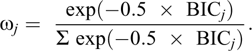
The BMA technique does not answer questions about robustness. The technique generates weights $ω_{j}$ for $j$ models with the posterior probabilities written by the commenter as:

ω_{j} = \frac{exp (- 0.5 \times {BIC}_{j})}{Σ exp (- 0.5 \times {BIC}_{j})} .

Few readers will have immediate intuition of what this formula does. When the commenter describes the method, it sounds like a modest reweighting of models to take into account the ${BIC}_{y}$ : “better fitting models are assigned a higher weight and thus have more influence on the results” (pp. 5-6). In practice, however, almost all the models are assigned a weight of zero, while one model is elevated to receive virtually all the weight. This is a weighted average of estimates in which almost all estimates are weighted to zero and excluded from consideration. As Yao, Simpson, and Gelman (2018:2) note, BMA “will asymptotically select the single one model” that offers a maximum fit with Y.

This pattern of essentially selecting a single model is seen clearly in the commenter’s Table 2, which shows a small-scale illustration of the model weighting procedure. Table 2 shows eight models with estimates ranging from −0.18 to +4.79. One model shows no evidence at all that gender is a factor in mortgage lending. Another model finds a five-percentage point higher mortgage approval rate for women over men (model 8). These models offer very different substantive conclusions, so the results clearly depend on how the model is specified. However, the commenter concludes that there is virtually no model variance, meaning that the results do not depend on decisions about which variables to include.

This robustness conclusion emerges because six of the eight regression estimates are given a weight of .000 and thus excluded entirely from consideration. Model 8, with the estimate showing the largest degree of gender disparity (in favor of women), is given 93.6 percent of the weight, and model 7 is given the remaining 6.4 percent of the weight, although the estimate is notably smaller. The difference in the $R^{2}$ between these models is .004 percent of explained variation in mortgage acceptance rates.⁴ Model 5, with completely contrary estimates, has a modestly lower $R^{2}$ but receives zero weight. Technically, the overall result is a weighted average across all models. But in reality, almost all the weights are zero. The procedure has simply selected the estimate from model 8, with a slight nod to model 7, and eliminated the other plausible models.

It is not credible to say one is considering eight plausible models, when six of them are given literally zero weight. The commenter claims that this approach is “easily justified in terms of basic probability theory” (p. 2). It is better described as a nonsense weighting of closely comparable models with no substantive justification at all. This is not model averaging or model robustness analysis—it is model selection. Moreover, it is not testing to see what happens if one of more of our modeling assumptions is wrong. It is just discarding models that do not maximize $R_{y}^{2}$ .

The commenter is aware that his method frequently deletes the results from every plausible model but one. He writes that the difference between YH and his method is mostly driven by “the extent to which the weights used for model averaging tend to concentrate on a single model” (p. 12). I agree this is a key problem: The commenter is doing model selection, while YH is doing model robustness.

Any approach which assigns 93.6 percent of the weight to the single model with the highest $R^{2}$ is essentially denying model uncertainty about the parameter estimate. Giving literally zero weight to a plausible alternative specification is extremely dogmatic. It is equivalent to saying that anyone who questions your result is wrong with nearly absolute certainty. This is completely contrary to the spirit of robustness analysis. As Winship and Western (2016) note, “even if we are individually confident about a particular specification, there are almost certainly others who will argue that we have gotten it wrong” (p. 646). The point of a robustness analysis is to allow other reasonable beliefs about model specification into the analysis. It should go without saying that this requires actually reporting the results from reasonable alternative specifications rather than deleting them before anyone gets a chance to see them.

Learning in Two Stages

In a sense, both YH and the commenter’s BMA are two-stage procedures, using the same first stage but diverging dramatically on the second stage. Both begin by generating a plausible model space and estimating all models to obtain a distribution of estimates.

At the second stage, the commenter’s BMA approach “learns from the data” by deleting the vast majority of the modeling distribution, leaving the estimate from the model with the highest $R^{2}$ as the model-averaged estimate. It is called model averaging, but in practice it is model selection. This may be a reasonable approach for predictive modeling, where the goal is simply to get a good prediction of the outcome, $\hat{y}$ . In practice, though, it would be regarded as rudimentary and far from the frontier of machine learning methods (e.g., Mullainathan and Spiess 2017). This is a model selection criteria that simply includes all variables that have a statistically significant partial correlation with y.

The second stage of YH, in contrast, proceeds to the influence analysis, which is a meta-regression showing which elements of the model space (such as which control variables) explain why different estimates are possible.⁵ Here, analysts learn from the data by unpacking the model assumptions and seeing which aspects of the model specification are critical to the results. This does not automate model selection, and it remains the responsibility of analysts to explicitly invoke and justify any model assumptions that are necessary to sustain their preferred result.

If one desired a model selection routine from YH, it would be based on the influence analysis. The selection criteria would be: All variables that significantly influence the treatment effect should be included, while others can be dropped (or not) without biasing the parameter estimate. This requires assuming that all the controls are strictly exogenous and that there are no other omitted variables or other specification errors. Sometimes authors and readers will be comfortable with that assumption, other times not. One can imagine an option that compares the full modeling distribution to the restricted distribution of results (including all influential controls) under the complete exogeneity assumption. Users can easily implement this approach after examining the influence results, and an example similar to this is offered in YH (p. 22, figure 3).

Conclusion

As Heckman (2005) has noted, there is no “assumption free” way to conduct an empirical analysis. It is not “embarrassing” to show that an analysis depends on certain assumptions. On the contrary, social scientists should be open and transparent about what assumptions are necessary for their conclusions. Today, too many empirical papers bury the evidence about which assumptions matter. Often, they bury model uncertainty in an effort to imply that their conclusions are true under all possible scenarios. Model uncertainty represents a limit to our knowledge that applied researchers are reluctant to admit.

Embracing transparency and showing what estimates are available—as well as which aspects of model specification affect the results—is central to thinking through the challenges of causal inference in a conditioning-on-observables analysis.

If a result is not robust to model specification, this does not mean we have failed to learn anything. Instead, it means we must focus on the influence analysis, which shows which model assumptions are needed for a strong conclusion. If those necessary assumptions are credible, authors should make an explicit case to readers justifying the model assumptions. We should not simply hide this information from readers, so they do not know that the results are dependent on key assumptions. And we should not hide this from readers by using opaque, scientific-sounding methods that delete the alternative models while claiming to average across them.

We need to guard against naive enthusiasm for more complex methods (Glaeser 2008). The YH method asks authors and readers to consider all the estimates that can be credibly supported by the data. This may strike some as too simple. But complex weighting schemes based on incorrect criteria are not an improvement. Methods which simply show the available estimates should not be rejected because they are easy to understand. As one philosopher put it, sometimes we can see a lot just by looking.

I wish to emphasize that the commenter arbitrarily limits his analysis and critique to the choice of alternative control variables, while the YH framework extends to alternative variable definitions (Brady, Beckfield, and Seeleib-Kaiser 2005), alternative cleaning and coding strategies (Leahey, Entwisle, and Einaudi 2003), alternative standard errors, data sources, and different estimation commands and functional forms (Kane et al. 2013). This, I believe, is the research frontier of robustness testing.

I am passionate about the potential of model robustness analysis to produce research that is more transparent and more convincing than current practices in sociology. The tremendous growth of computational power has given rise to serious problems of asymmetric information between analysts and readers (Young 2009). The result is a growing crisis of confidence in science today, owing to the fact that analysts, but not readers, can see and select a preferred estimate after running large numbers of similar models. We need better methods of showing what results are possible under a reasonable set of model assumptions. YH worked hard to develop a robustness command that would be easy to use and can perform transparent robustness analysis across many aspects of model specification in a wide range of empirical settings. The project is ongoing (Stewart and Young 2018; Young 2018; Muñoz and Young 2018), and I welcome input and ideas on how to make it better and more useful. However, a proposal that casts aside the objectives of robustness analysis and conducts single model selection based on the $R^{2}$ is working on a different endeavor.

Footnotes

Acknowledgment

The author would like to thank Michelle Jackson, Sheridan Stewart, John Muñoz, and Katherine Holsteen for helpful feedback and suggestions.

Declaration of Conflicting Interests

The author(s) declared no potential conflicts of interest with respect to the research, authorship, and/or publication of this article.

Funding

The author(s) received no financial support for the research, authorship, and/or publication of this article.

Notes

References

Acharya

Avidit

Blackwell

Mathew

Sen

Maya

. 2016. “Explaining Causal Findings without Bias: Detecting and Assessing Direct Effects.” American Political Science Review 110(3):512–29.

Athey

Susan

Imbens

Guido

Wager

Stefan

. 2017. “Approximate Residual Balancing: De-biased Inference of Average Treatment Effects in High Dimensions.” Working Paper No. arXiv:1604.07125, Stanford University, Stanford, CA.

Belloni

Alexandre

Chernozhukov

Victor

Fernández-Val

Ivan

Hansen

Christian

. 2017. “Program Evaluation and Causal Inference with High-dimensional Data.” Econometrica 85:233–98.

Belloni

Alexandre

Chernozhukov

Victor

Hansen

Christian

. 2014. “Inference on Treatment Effects after Selection among High-dimensional Controls.” Review of Economic Studies 81(2):608–50.

Brady

David

Beckfield

Jason

Seeleib-Kaiser

Martin

. 2005. “Economic Globalization and the Welfare State in Affluent Democracies, 1975-2001.” American Sociological Review 70:921–48.

Clarke

Kevin

. 2005. “The Phantom Menace: Omitted Variable Bias in Econometric Research.” Conflict Management and Peace Science 22(4):341–52.

Cole

Stephen

Platt

Robert

Schisterman

Enrique

Chu

Haitao

Westreich

Daniel

Richardson

David

Poole

Charles

. 2009. “Illustrating Bias due to Conditioning on a Collider.” International Journal of Epidemiology 39:417–20.

Doppelhofer

Gernot

Weeks

Melvyn

. 2009. “Jointness of Growth Determinants.” Journal of Applied Econometrics 24:209–44.

Elwert

Felix

Winship

Chris

. 2014. “Endogenous Selection Bias: The Problem of Conditioning on a Collider Variable.” Annual Review of Sociology 40:31–53.

10.

Glaeser

Edward

. 2008. “Researcher Incentives and Empirical Methods.” Pp. 300–319 in Foundations of Positive and Normative Economics: A Handbook, edited by Caplin

Andrew

Schotter

Andrew

. Oxford, England: Oxford University Press.

11.

Google. 2017. “Our focus on pay equity.” Retrieved March 13, 2018 (https://www.blog.google/topics/diversity/our-focus-pay-equity/)

12.

Greene

William

. 2012. Econometric Analysis. 7th ed. Upper Saddle River, NJ: Prentice Hall.

13.

Hansen

Bruce

. 2005. “Challenges for Econometric Model Selection.” Econometric Theory 21:60–68.

14.

Heckman

James

. 2005. “The Scientific Model of Causality.” Sociological Methodology 35:1–97.

15.

Hofman

Jake

Sharma

Amit

Watts

Duncan

. 2017. “Prediction and Explanation in Social Systems.” Science 355:486–88.

16.

Kane

Jennifer

Morgan

Philip

Harris

Kathleen

Guilkey

David

. 2013. “The Educational Consequences of Teen Childbearing: Comparisons across Ordinary Least Squares Regression, Propensity Score Matching, Parametric and Semi-parametric Maximum Likelihood Estimation.” Demography 50:2129–50.

17.

Ley

Eduardo

Steel

Mark

. 2007. “Jointness in Bayesian Variable Selection with Applications to Growth Regression.” Journal of Macroeconomics 29(3):476–93.

18.

Leahey

Erin

Entwisle

Barbara

Einaudi

Peter

. 2003. “Diversity in Everyday Research Practice: The Case of Data Editing.” Sociological Methods and Research 32(1):64–689.

19.

Mullainathan

Sendhil

Spiess

Jann

. 2017. “Machine Learning: An Applied Econometric Approach.” Journal of Economic Perspectives 31(2):87–106.

20.

Muñoz

John

Young

Cristobal

. 2018. “We Ran 9 Billion Regressions: Eliminating False Positives through Computational Model Robustness.” Sociological Methodology, 48, 1–33.

21.

Morgan

Stephen

Winship

Christopher

. 2007. Counterfactuals and Causal Inference: Methods and Principles for Social Research. Cambridge, England: Cambridge University Press.

22.

Nyhan

Brendan

Montgomery

Jacob

Torres

Michelle

. 2017. “How Conditioning on Post-Treatment Variables Can Ruin Your Experiment and What to Do About It.” American Journal of Political Science. Retrieved March 30, 2018 (https://doi.org/10.1111/ajps.12357).

23.

Rosenbaum

Paul

. 1984. “The Consequences of Adjustment for a Concomitant Variable that Has Been Affected by the Treatment.” Journal of the Royal Statistical Society. 147(5):656–66.

24.

Shmueli

Galit

. 2010. “To Explain or to Predict?” Statistical Science 25(3):289–310.

25.

Slez

Adam

. 2018. “The Difference between Instability and Uncertainty: Comment on Young and Holsteen (2017).” Sociological Methods and Research.

26.

Stewart

Sheridan

Young

Cristobal

. 2018. “Functional Form Robustness.” Working Paper, Stanford University, Stanford, CA.

27.

Winship

Christopher

Western

Bruce

. 2016. “Multicollinearity and Model Misspecification.” Sociological Science 3:627–49.

28.

Yao

Yuling

Vehtari

Aki

Simpson

Daniel

Gelman

Andrew

. 2018. “Using Stacking to Average Bayesian Predictive Distributions.” Bayesian Analysis. Retrieved January 16, 2018 (https://projecteuclid.org/euclid.ba/1516093227).

29.

Young

Cristobal

. 2009. “Model Uncertainty in Sociological Research: An Application to Religion and Economic Growth.” American Sociological Review 74(3):380–97.

30.

Young

Cristobal

. 2018. “Model Uncertainty and the Crisis in Science.” Socius: Sociological Research for a Dynamic World 4:1–7.

31.

Young

Cristobal

Holsteen

Katherine

. 2017. “Model Uncertainty and Robustness: A Computational Framework for Multi-model Analysis.” Sociological Methods and Research 46(1):3–40.