Some Methods for the Analysis of Event Sequence Data from Multiple Respondents

Abstract

The analysis of sequence data poses a great challenge; existing methods for the comparison of sequences take what theoretical grounding they have from other fields (most importantly, genetics). We argue that set theory provides a way of establishing the relations between sequences that has a natural application to the case in which the sequences are orderings of a set of events, all compatible with an underlying partial order shared by multiple respondents. We also examine the possibility that observed differences in sequence data come from a stochastic process in which some events are poorly ordered because respondents cannot discriminate between them. We show that such methods shed light on several quantities that have been of interest to researchers, such as the degree of consensus within a group as to ideal sequences, the degree of respondent accuracy in reporting, and the degree to which plans and reality coincide.

Keywords

sequences event partially ordered sets poset algebraic

Phenomena which are limited to a certain number of individuals either must be treated as complex and analyzed into elementary and universal elements, or, if this variation cannot be done, then their content, varying with the variation of social milieu, must be omitted and only the form of their occurrence reconstructed.

—Thomas and Znaniecki, The Polish Peasant (1918:26).

A common criticism of conventional formal analysis in sociology is that it eschews our core theoretical foci of relations and dynamics and privileges an imagination of simultaneous within-individual causation (e.g., Abbott 1998). For this reason, there has been a great deal of enthusiasm for techniques that seem to push in the opposite direction. One family of techniques that combines both dynamism and relationality consists of methods for the analysis of sequences of events.

Within this broad class, there is a stark division between two families of approaches, which correspond to the two great philosophies of time in the modern West, the Cartesian and the Leibnizian. The Cartesian begins with the empty canvas of space-time; time is thus conceived of as an ordered infinite set of real numbers onto which beginnings and endings can be dropped. The Leibnizian conception, in contrast, begins with events and their relations; time is induced by the structure of the relations between events, and not vice versa. Were there no events, there would be no time. The Cartesian approach lends itself naturally to the sorts of parametric models that dominate social science, and, in particular, it dovetails smoothly with frequentist probabilistic reasoning. Such an approach certainly can be used to establish complex relations between events, if the events are noninstantaneous (e.g., Moody 2002). However, it also fits well into the wider class of linear models, where the duration until an event occurs for some case is a dependent variable regressed on a function of a set of covariates.

The Leibnizian approach, in contrast, lends itself naturally to algebraic approaches or to related formalisms that are taken from network analysis (e.g., see Abell 1993; Bearman, Faris, and Moody 1999; Smith 2007). For this reason, there have been repeated bursts of enthusiasm (invariably leading to disappointment) that methods appropriate for social networks can be transferred, with little modification, to structures of temporally bound data. In particular, there have been a number of creative attempts to develop or adapt nonparametric techniques to analyze such events.

Much of the work in sociology on the similarity of sequences has come from the application of methods of sequence comparison that were developed for genetic analysis (for a review, see Cornwell 2015). In the original genetic context, not only are the sequences (usually) of the same length, and with a very restricted number of elements, but the biochemical processes leading to change could be plausibly modeled, leading to a set of reasonably countable differences between sequences. Unfortunately, the application of this logic to social sciences has been strained (Wu 2000), and the success of methods based on the assumption that such measures could be used to find clusters of sequences has been far from overwhelming (Warren et al. 2015).

We believe that the reason for this limited success is that current approaches to analyzing sequences of events have attempted to ignore the particularities of the relevant data generation regimes (also see Halpin 2010). Thus, in some data sets, there are a fixed number of slots for events to take place (e.g., an employee may receive a new assignment every fall), and in others, events occur sporadically (e.g., promotions). In some data sets, there is a fixed order to all events (as in military promotions), while in others, events can come in any order (e.g., the birth of boys as opposed to girls). In some data sets, events may be repeated or never occur (e.g., being the victim of a crime), while in others, every event can only happen once (e.g., military promotions), and in still others, every event must happen once and only once (e.g., death). Finally, in some data sets, all subjects share the same set of events (e.g., respondents ordering events that took place in a jointly experienced history; or promotions of a set of persons sampled from the highest rank attained), while in others, respondents have disjoint sets of events (e.g., promotions of a set of persons sampled as an initial cohort). The notion that the same techniques would be applicable across all these different regimes of data gathering demonstrates a Panglossian optimism, and the implausibility of this optimism is sufficient to explain the limited success of many explorations, as well as the interest in adapting the basic procedure to deal with the particularities of the data collection regime (e.g., Hollister 2009).

Different theoretical questions will of course guide what we consider to be of central methodological concern in any specific undertaking. However, we can shed some light on the types of methodological approaches by distinguishing between the form and the content of any sequence of events. Given a sequence of events a, b, b, b, c, d, and c, we may consider the unordered set {a, b, c, d} to capture the content of this sequence. The form is the arrangement over the seven places.¹ This sequence shares the same content as the formally different sequence a, b, c, d, d, and d. And it has something formally similar to the sequence e, f, f, f, g, h, and g, which has a wholly different content. It is our belief that it is difficult to interpret the results of methods that jointly examine the form and the content of sequences. If there is particular interest in sequences (and not mere occurrence of events), this suggests that we might focus our attention of methods that concentrate on the form that could be put on a set of events, and not the content.

It would of course be of great interest to develop methods that can extract formal similarities even across cases that differ in content. And it may well be possible to develop these for specific data collection regimes. But outside of that, we think that a useful step would be the development of approaches concentrate on differences in form and that can be applied to data in which there is no variation in content.

We therefore here propose a new approach that may be useful for one particular type of data on events—data in which the same events are arranged into different ordered sequences—leading to highly interpretable numerical results. We focus on the fact that some (but not necessarily all) pairs of events are ordered such that one precedes the other. We then use this fact to develop some simple indices of the degree of overlap in different sequences, and, finally, go on to demonstrate ways of quantifying the agreement across a larger group. We do not pretend that this method can serve as a general framework to handle all forms of event sequence data. However, given the a priori plausibility of this approach, and its close connection to well-understood aspects of set theory, aspects which have a natural affinity to our conceptions of events, these methods seem worthy of sustained attention.

An Algebraic Approach

Sets of Events

Consider data of the following form: All respondents are given the same set of K events and asked to order them in time. Examples of such data arise when we see how different subjects recall a complex of historical events (Smith 2007) or when we ask partners separately about the order in which certain events transpired in their romantic relation.

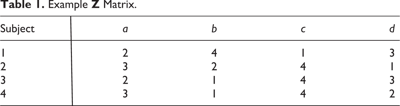
We will assume that the data come in an N × K matrix Z in which z_ij = r, meaning that the ith respondent assigns the jth possible event to position (or rank) r. Thus, every row of data is a permutation of the series of the first K natural numbers. (We here exclude the possibilities of missing values and of ties.) For example, consider data from four respondents (N = 4) ranking four events (K = 4) thusly: (cadb), (dbac), (bacd), and (bdac). This produces the following Z matrix (see Table 1).

Table 1.

Example Z Matrix.

Subject	a	b	c	d
1	2	4	1	3
2	3	2	4	1
3	2	1	4	3
4	3	1	4	2

Such data have been analyzed in a large number of important and creative ways (see, importantly, Coombs 1964; for some applications, see Coxon and Jones 1978). However, there is a conceptual difference between certain data tasks that may produce the same sort of data. In some cases, such as when respondents might be asked to place certain events in a logical order (a task often used in psychological testing), we imagine the core process as directly reflected in the ordinal characteristics of the sequence. However, in other tasks, such as where a set of respondents are asked to order historical events, we may find that they only have pockets of ordering and that the overall sequence produced may have arbitrary components. Finally, in other cases, for example, when respondents are asked to rank a set of objects (e.g., sociology departments) in quality, we expect that the objects actually have positions on some sort of interval quality metric such that it is in principle possible (if unlikely) for two objects to have the same value. The respondents, uncertain of the interval scores, can still complete the ranking task, but possibly with some degree of error where objects are close in quality.

Most approaches to sequenced data have assumed, with little justification, that the respondent’s relation to the data is that of a deterministic and unilinear ordering—akin to the notion of a “Guttman scale” in which all items can be deterministically ranked (Guttman 1950). This would be appropriate to data collected under the first of the three regimes discussed above (logical order). But, as pointed out by Wiley and Martin (1999), there are two ways that we can imagine relaxing this assumption. One is to retain determinism in the binary relation between items, but to allow for a partial ordering (defined below), in which some pairs of items are unordered. For example, recounting the history of the American Revolution, respondents might know that the Boston Massacre came before Valley Forge and that the Boston Tea Party came before the Declaration of Independence, but be completely unsure as to the relation between the military events and the political events. The relations that do exist are therefore deterministic (the Tea Party definitely came before the Declaration), but not all pairs of events have a relation.

A second way of relaxing the assumption of a deterministic order is to propose that a lack of order comes not because certain events are intrinsically incomparable but simply that they are difficult to compare. For example, our memories are imperfect even in the best of times, and, to arrange our memories in an order, we may use heuristics that do not work for all pairs of events. Thus, a respondent answering a survey on drug use might be confident that he had tried cigarettes and beer before trying marijuana, and marijuana before trying cocaine or Quaaludes, because he associates the first two with junior high school, the third with high school, and distinctly remembers the final two as being after he acquired a driver’s license. The events that are closer in time are harder to order. We might therefore allow for a stochastic response process; this is the logic behind the Rasch (1966) model. We pursue both of these relaxations here.

Fundamental Definitions

The core of our approach is to treat each sequence as an ordered set of elements. This ordering is due to temporal precedence, such that we say that either one event precedes another, or it does not. Two events are said to be “incomparable” if neither precedes the other. Two events are said to be “identical” if each precedes the other (i.e., simultaneous events are the same event; we here assume without loss of generality that all events are distinct). We therefore can apply basic notions from algebraic set theory to develop some formal procedures of analysis. We begin with some conventional definitions and then show how these can be used to shed light on social data.

A binary relation on some set δ = {δ₁, δ₂, δ₃,…} is a subset of all ordered pairs of the members of δ. Thus, a binary relation is itself a set of sets, and therefore, binary relations can be operated on just as other sets. A “partially ordered set” (or “poset,” for short) is a set of elements {δ₁, δ₂, δ₃,…} and a binary relation denoted ≤, which satisfies the following three conditions:

reflexivity: δ₁ ≤ δ₁;

antisymmetry: δ₁ ≤ δ₂ and δ₂ ≤ δ₁ implies δ₁ = δ₂; and

transitivity: δ₁ ≤ δ₂, δ₂ ≤ δ₃ implies δ₁ ≤ δ₃.

Consider a poset A, consisting of elements δ₁, δ₂, δ₃, and so on, together with a binary relation ≤; this may be denoted A = {δ, ≤}. A is a “chain” if for any δ₁ and δ₂, either δ₁ ≤ δ₂ or δ₂ ≤ δ₁ (i.e., A is “complete”). A is an “antichain” if there is no δ₁ and δ₂ such that δ₁ ≤ δ₂. Note that a poset A can be expressed as a Boolean matrix A in which a_ij = 1 iff δ _i ≤ δ _j in A. The “dual” of a poset A (={δ, ≤ _A }) is a poset B such that (δ₁ ≤ _A δ₂) ⇔ (δ₂ ≤ _B δ₁) (Trotter 1992:4).

It will be noted that a “sequence” of events, as generally termed in the sociological literature, is a chain (also called an “order”). Much of the interest in the social sciences has involved an attempt at the comparison of sequences derived from social data. In some cases, we are interested in comparing sequences from the same person (e.g., ideal and real sequences; Frye and Trinitapoli 2015; Soller 2014). In other cases, we are interested in comparing sequences from a large number of persons, either for dyadic comparison or aggregation of dyads (Frye and Trinitapoli 2015; Harding 2007; Soller 2015). From such comparison, we may also generate inductive typologies and classify actors based on their similarity (e.g., career sequences; Stovel, Savage, and Bearman 1996).

Any poset can be displayed as a “Hasse diagram,” a graph in which an arrow between two events implies that the origin of the arrow precedes the destination, and in which no transitively implied relations are drawn. Thus, in the first row of Table 1 (the leftmost chain in Figure 1), because c comes first, it precedes not only a but also b and d. However, these last two relations need not be explicitly displayed. Since c precedes a and a precedes b, we know that c must precede b, and ditto for d. Here, in keeping with algebraic convention, time flows upward, as precedence relations go from low to high. The four rows in Table 1 can then be portrayed as shown in Figure 1.

Figure 1.

Four chains from Table 1.

Thus, our data matrix Z may be understood as a set of chains, one for each respondent. It can equivalently be seen as a set of matrices. From these data, for the ith respondent, we can compute a matrix X ⁱ with values as follows:

x_{j k}^{i} = In (z_{i j} < z_{i k}),

where In() is the indicator function. Note that X ⁱ is a Boolean matrix (values are either 0 or 1), that xⁱ _jk + xⁱ _kj = 1 (k ≠ j), and that X ⁱ is a chain, which implies that the row and column sums are each a permutation of the series of the first K natural numbers (i.e., going from 1 to K). For example, the X ⁱ matrix for the first row of the Z matrix given as Table 1 is given in Table 2. Note that the row (column) sums indicate the rank of any element in the sequence from early (late) to late (early).

Table 2.

Example X ⁱ Matrix.

Subject	a	b	c	d	Sum
a	1	1	0	1	3
b	0	1	0	0	1
c	1	1	1	1	4
d	0	1	0	1	2
Sum	2	4	1	3

Consider the case in which two (or more) different persons are reporting on the same sequence or that in which we are interested in comparing a person’s ideal sequence to a realized one. We wish to quantify the degree of overlap between these sequences or, equivalently, the underlying orders. Unlike other approaches to this problem, which have imported solutions taken from particular domains that do not necessarily have any relation to the structure of events, here we base our mathematization only on the logic of events that have relations of precedence (for a recent application using partial orders of events, see Breiger and Smith 2018).

Such an approach was previously taken by Elzinga (2003), who uses the logic of precedence to develop a general approach for quantifying the degree of (dis)similarity between any two sequences in terms of the overlap of their precedence relations. Here, Elzinga does not restrict attention to dyadic precedence relations but to all unique subsequences. This method, like most others, deliberately attempts to be applicable to all forms of sequences yet also appeals to intuitive judgments to validate its results. Yet it seems to us that our intuitive judgments of closeness and distance will depend on the nature of the data in question. For example, Elzinga (2003:15) suggests that it is apparent on the face of it that OM methods are problematic because they fail to recognize that the sequence {1, 2, 3, 4, 5, 6, 7, 8} is closer to that of {1, 1, 2, 3, 4, 5, 6} than it is to {1, 2, 3, 4, 5}. However, if these data were on the school grades experienced by children, and the end of each sequence came via censoring, we might doubt that the first two sequences were similar, since one indicates a normal progression, and the second being “left back.”

Elzinga’s approach, then, has an advantage in being applicable to cases in which there are differences in content,² but suffers from the correlative drawback of needing to make stronger theoretical assumptions about which sequences are more like one another. Here, in contrast, we sacrifice breadth of applicability (and the capacity to compare sequences in terms of their complexity; here, see Elzinga 2010) for clearer interpretation and fewer arbitrary decisions. We give more terminology, illustrate through an analysis of Table 1, and then turn to some actual data.

Similarities of Sequences

With more algebraic terminology, we can quantify the similarity of two or more sequences. The “width” of a poset A is the cardinality of the maximal antichain B such that B ⊆ A. The “height” of a poset A is the cardinality of the maximal chain B such that B ⊆ A. For two individuals (or other observed units), i and i*, let $X^{ii *}$ = X ⁱ ∩ X^i* (i.e., it is the intersection of the two chains). Note that if X ⁱ and X^i* are duals, then X^ii* is an antichain, and hence has width K and height 1, while if X ⁱ = X^i*, then X^ii* is a chain, and hence has width 1 and height K. Accordingly, either the width (negatively) or the height (positively) is a decent indicator of the degree of agreement between i and i* in terms of their ordering of the event set. The width indicates the maximal number of elements that, at any point in the sequence, cannot be ordered, and may be taken as an indicator of temporal ambiguity. The height indicates the longest agreed-upon subsequence and may be taken as the degree of narrative development.

Thus, the width and height are not mirror images. Maximizing one is not always minimizing the other. Consider two archetypical shapes, a cross (+) and a square (□). Imagine each of these as a rough representation of the Hasse diagram of a partial ordering; to give a very small illustration of each, the first might consist of relations δ₁ ≤ {δ₂, δ₃, δ₄} ≤ δ₅ and the second δ₁ ≤ δ₂; δ₃ ≤ δ₄. The first has a relatively large height (3) but also a large width (3). That is, although there are some elements that are incomparable, they sit at a particular place in the sequence, and there is still a large chain present. The second has both a moderate width and a moderate height (both 2); although any point in the sequence, there are not many incomparable elements, we find such incomparability at multiple points over the course of the structure. Thus, whether we attempt to maximize height or minimize width depends on whether we prefer to maximize the elaboration of our story overall or maximize the clarity at all points in the story.

Further, for some purposes, we may not be interested merely in the width, which is the maximal disagreement, but in the areas of maximal agreement. To do this, we first introduce the notion of an “incomparability graph.” A graph G is a set of nodes N and edges E, which are a subset of all ordered pairs of elements in N; note that a poset may also be considered a (directed) graph. Given two elements, δ₁ and δ₂, in a poset, we say that δ₁ and δ₂ are incomparable if (not δ₁ ≤ _A δ₂) and (not δ₂ ≤ _A δ₁). Given a poset A, the incomparability graph of A, denoted S(A), is a graph = (A, E) in which the elements are the elements of A and for some a, b ∈ A, (a, b) ∈ E iff (not δ₁ ≤ _A δ₂) and (not δ₂ ≤ _A δ₁). For any node n in a graph G, we denote the degree of n as d^G(n). We call δ₁ in A part of the “waist” if there is no δ₂ in A such that d^S^(A)(δ₂) < d^S^(A)(δ₁). We call δ₁ a “wasp waist” if d^S^(A)(δ₁) = 0. Respective of any wasp waist, A can be portioned into two sets, the “abdomen” which consists of all elements that precede the waist, and the “thorax,” which consists of all elements that succeed it. Thus, if X^ii* has a wasp waist, the respondents agree as to the portioning of the sequence into theoretically crucial before (abdomen) and after (thorax) subsets.

It may be of interest to introduce one last quantification of a poset, namely its dimensionality. An “extension” of some poset A (={δ, ≤ _A }) is a poset B ={δ, ≤ _B } such that A ⊆ B, or (δ₁ ≤ _A δ₂) → (δ₁ ≤ _B δ₂). Hence, if B is an extension of A, we can say that A ≤ B. For any A and B that share a set of elements δ, we can say A ∩ B = {δ, ≤ _AB }, where (δ₁ ≤ _AB δ₂) iff (δ₁ ≤ _A δ₂) and (δ₁ ≤ _B δ₂). If we have some set L of posets {L₁, L₂,…, L_D}, we can denote L₁ ∩ L₂ ∩ L₃∩…∩ L_D parsimoniously as ∩L. If we represent our posets as Boolean matrices, we say AB = A ∩ B iff ab_ij = a_ijb_ij. If some B that is an extension of some A is a chain (as defined above), B is said to be a “linear extension” of A. Note that B is therefore an order representing one permutation of the elements {δ}. The “dimension” D of a poset A is the smallest integer such that there is a set L of D linear extensions {L₁, L₂,…, L_D} of A such that A = ∩L (Trotter 1992:8; Pretzel 1977). L is then known as a “realizer” of A. It is well-known that the dimensionality of any poset is less than or equal to its width. One implication is that a poset of dimensionality D could arise as a result of the combination of D different orders, an interesting possibility for the exploration of aggregate data to which we refer below.

Stylized Example

We here propose to the use the width and height of the poset formed by the intersection of two or more chains as measures of the agreement in sequences. Such measures may be more interpretable than other ad hoc measures, especially those based on rank correlation, which will not be closely related to the underlying cognitive processes if these involve a combination of strict ordering and total indifference. For example, let us return to the data in Table 1. Note that P1s and P4s orders are dual, which means that their intersection is an antichain. Two other intersections are graphed in Figure 2, that of P1 and P2 on the left, and P2 and P3 on the right. P2 agrees with P3 about everything except how to fit d into the sequence but disagrees with P1 about everything except that d should precede b. Note that the height of the first poset is 2, while that of the second is 3; contrariwise, the width of the first poset is 3, and that of the second is two. The results of all comparisons are in Table 3(a) and (b).

Figure 2.

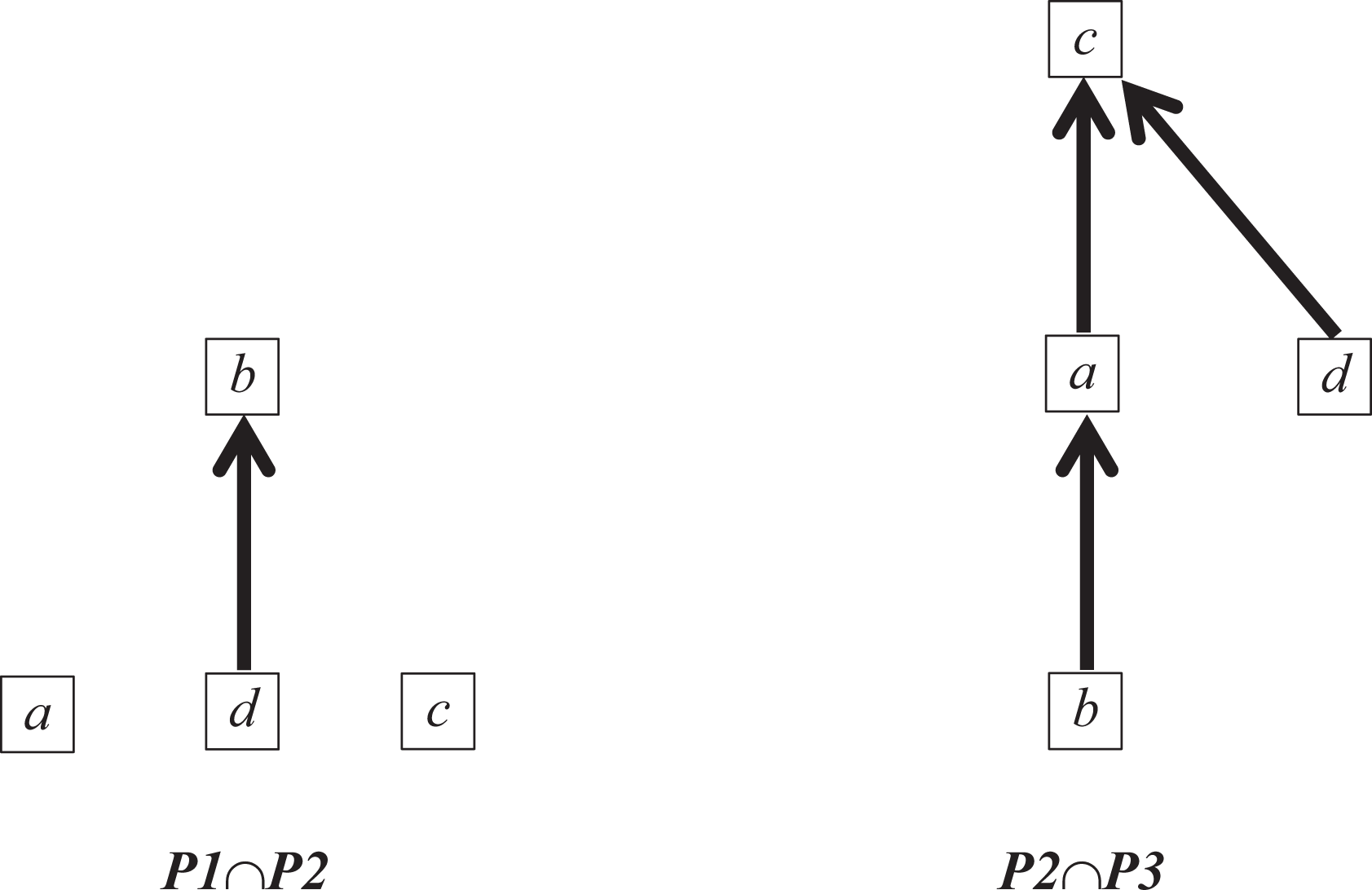
Two intersections of rows from Table 1.

Table 3.

Results of Intersections of Rows from Table 1; (a) Height and (b) Width.

Subject	P1	P2	P3	P4
(a) Height
P1	4	2	2	1
P2	2	4	3	3
P3	2	3	4	3
P4	1	3	3	4
(b) Width
P1	1	3	3	4
P2	3	1	2	2
P3	3	2	1	2
P4	4	2	2	1

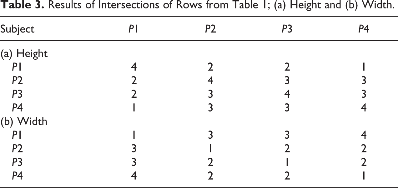
This suggests that, thinking from the perspective of each case serially, P1 is least like P4, while both P2 and P3 are least like P1, and P4 is least like P1. The set of relations can be plausibly expressed in a two-dimensional space as shown in Figure 3, where distances in the figure are monotonically related to differences between sequences. Thus, P1 appears to have a very divergent conception from the others, and this might be used to partition the set. However, if P1 and P2 were, say, reporting on the same objective sequence of events (as they would if they had jointly experienced the same sequence and were now attempting to recreate it), as were P3 and P4, reporting on their shared experiences, we would say that the first pair seem disagree more as to their memory of the ordering of these events than does the second pair (and the other values in this table would be meaningless). We go on to illustrate how this basic approach can be used to approach a number of common problems in the analysis of sequence data using a set of interesting data.

Figure 3.

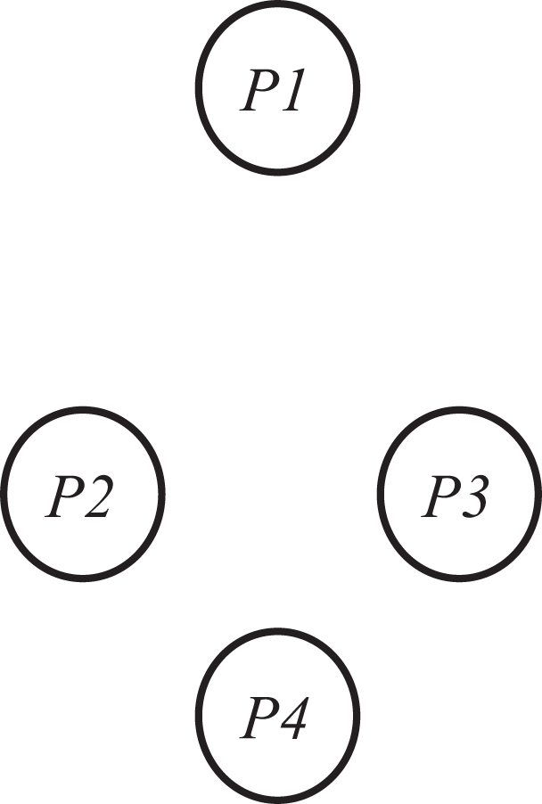
Spatial representations of distances from Table 3(b).

Illustrative Analyses

Data

Over the past decade, sociologists concerned with romantic and sexual behavior during adolescence and young adulthood have taken a sequential turn. Rather than treating behaviors (e.g., sexual debut or contraceptive use) in isolation, they attempt to place them in the context of surrounding events in a relationship. This research has relied upon optimal matching techniques to operationalize (a) concordance between idealized and actual relationships (Frye and Trinitapoli 2015; Soller 2014, 2015) and (b) normative consensus about romantic relationships among adolescents in the same social context (Harding 2007; Soller 2015).³

This interest in romantic sequences has been fueled by instruments on the National Longitudinal Study of Adolescent Health (Add Health). This is the data used by Soller; further, these instruments served as a template for the studies of Frye and Trinitapoli (2015). We ourselves draw upon waves 1 and 2 of Add Health.

In the wave 1 administration, respondents were presented with a set of actions and asked to pick those that would happen in their ideal next romantic relationship. Subsequently, respondents were asked to place the selected actions in the order they would want them to occur. In the second wave, approximately 12 months later, respondents were asked to perform the same task (with only minor alterations to the wording of available actions) for their three most recent romantic relationships. We refer to these data as the “ideal” and “real” sequences, respectively.

For illustrative purposes, we analyze only eight events. These are Go on Group Date, Hold Hands, Go on Date Alone, Kiss, Meet Parents, Discuss Birth Control, Tell Others We’re a Couple, and Have Sex. (See Online Appendix A for the precise wording of these and other items analyzed.) We eliminated events for which the wording was changed between the ideal and real versions, or between the two waves, and those (e.g., Get Pregnant) that few students experienced.

It is important to emphasize that we only analyze the subjects who reported all of these events as part of their ideal and/or real sequence (depending on the analysis in question). Our number of respondents therefore changes depending on the analysis and is substantially smaller than the entire set of students who completed the relevant parts of the interview. Because of our deliberate exclusion of variation in the content of events, our results are not directly comparable to methods that attempt to examine both difference in content and form of events, but we do point to some interesting relations between our results and others. We will first demonstrate the application of relaxing the assumption of deterministic orders to that of deterministic partial orders. We use this approach to quantify the agreement in sequences such that the results can be used as covariates in individual-level and dyadic-level models; we then attempt to ascertain groups of respondents who share partial orders. We then turn to relaxing the assumption of deterministic orders by allowing for a stochastic response process and use this to group respondents into clusters who share placements of the events in an underlying metric.

Differences between Ideal and Real Sequences

One set of interesting theoretical questions pertains to the disjunction between the ideal sequence expressed at the first wave and the actual sequence of a relationship that transpired between this time and the measurement at the second wave. In particular, Soller (2014) argued that the difference between girls’ ideal relationships and those that came closest on the heels of their filling out the wave 1 form (“inauthenticity”) was related to worsening psychological distress. We believe that Soller’s fundamental theoretical argument is correct but that the method of optimal matching he used, which blends form and content, leaves us uncertain as to whether or not this distress may be due to simply to the fact that many girls had longer sequences than they had anticipated—and longer sequences are more likely to involve sexual activity that girls may regret, or whether it might be due to differences in form. Although our choice of eight events is only one possible set of content-invariant observations, we use it as an illustration of how to pursue a wholly formal investigation.

The width and height of a partial order can be used to examine the agreement between respondents answering the same item, or the agreement within a respondent across items. Here, we examine the latter first, by combining each respondent’s ideal and real orders to make a partial order; the wider (higher) the resulting poset, the less (more) agreement there is between the two. We use these to ascertain the support for Soller’s theory. We also, for illustrative purposes, compare to the distance via optimal matching (with substitution costs determined empirically from the subset of the data used). First, we may be interested in whether there is a gender difference in terms of the degree to which students’ reality matched their ideals, thereby treating characteristics of this poset as a dependent variable. To do this, we must restrict our attention here to 11th graders who have all eight of our steps listed in wave 1 ideal and had experienced all these steps in at least one relationship they discussed later in wave 2, a set of 465 students. We then use the poset characteristics as predictors of depression. Following Soller, we employ a scale of items on negative affect (at wave 2), basically tapping “feeling down” or depression (see Online Appendix A for wordings).

First, is there evidence that the girls have a greater discrepancy between real and ideal sequences than boys? Table 4(a) suggests not; indeed, the disjunction is a bit in the other direction: The real sequences were closer to the ideals for girls than for boys. However, the differences are minor, and of marginal significance at best. It is worth noting that we find similar insignificance using the distance from the Optimal Matching algorithm.

Table 4.

(a) Mean Ideal-real Agreement by Sex and (b) Correlations with Psychological Distress by Sex.

	Height	Width	OM Distance
(a) Mean ideal-real agreement by sex
Boys (N = 205)	4.09	3.67	5.51
Girls (N = 260)	4.28	3.24	5.26
t Test	[p = .060]	[p = .098]	[p = .221]
(b) Correlations with psychological distress by sex
Boys (N = 205):	−.02 [p = .777]	.06 [p = .37]	.04 [p = .557]
Girls (N = 260):	−.16*	.10	.18*
	[p = .011]	[p = .119]	[p = .003]

*p < .05.

Second, does the discrepancy between ideal and real sequences predict depression? Table 4(b) demonstrates that it does for girls, at least, when we use the measure of height. (The correlation for width is in the right direction, but smaller and statistically insignificant.) It is perhaps interesting that the correlation between height and distress is nearly identical to that reached when we use the optimal matching distance instead.

The relation between disagreement of real and ideal sequences here has been restricted to cases in which all cases experience all events. This should be understood, therefore, as a very conservative test of the hypothesis of inauthenticity (since that theoretical argument does not restrict itself to formal differences). It should be noted that for these data, the vast amount of variance is necessarily found between sequences of different lengths, and not within sequences.⁴ Thus, even though these are simple bivariate relations, they are intriguing, if not determinate, and suggest that Soller’s claims apply not only to the difference in content between ideal and real sequences.

Hierarchical Agglomeration

One of the most frequently sought applications of sequence analysis involves taking a set of individual sequences and attempting to determine a smaller set of idea-typical clusters (e.g., Aisenbrey and Fasang 2017; Cornwell and Warburton 2014; also see Fasang and Liao 2014). We go on to demonstrate how our approach can be used to uncover clusters of persons who may be parsimoniously noted as sharing a common partial order, even though their original data come in the form of different orders.

We do this by constructing an agglomerative clustering routine. We begin with each distinct row in the data matrix Z weighted by the number of observations which fall into this pattern. We first order the different indices we have in terms of priority: Here, we use the total number of precedence relations in a poset X ⁱ (which we will denote r(X ⁱ )), the width w(X ⁱ ), and the height h(X ⁱ ), in this order. As before, X^ii* = X ⁱ ∩ X^i*, with N^ii* the number of individuals in both rows, but note that X ⁱ and X^i* now need not be chains. Denote whichever function we are looking at as f(), scored so that increasing values are increasing badness (thus r and h are inverted, but not w). For any f(), we construct a penalty function for the loss of parsimony associated with collapsing rows i and i*:

Penalty (f (X^{i i^{*}})) = {N_{i i *}}^{g} (f (X^{i i^{*}})) - {N_{i}}^{g} (f (X^{i})) - {N_{i *}}^{g} (f (X^{i^{*}})) .

Given that there is no obvious reason why our penalty function should scale linearly with the number of observations in a row, we allow for flexibility in specifying this relation by specifying an exponent g for each frequency weight; here, we set g to 1 for our example results.

We choose whichever pair of rows minimizes this function; in the example shown, we use all three functions. In other words, in the case of a tie with f = r, we proceed to minimize the w penalty, and, if that also leads to a tie, we go on to consider the h penalty. The aggregated rows then become a cluster with an aggregate N, then considered available for further aggregation in future rounds. Our goal is to produce maximally constrained structures, which means, above all else, that they have the fewest incomparabilities.

To stick with the empirical application we have considered so far, we may consider each respondent’s ideal sequence of a set of events in a romantic relationship to be what Gagnon and Simon (1973) called a “script.” Our clustering approach attempts to see whether scripts form families of “meta-scripts” that share important features. We therefore applied the clustering as described above to a subset of the Add Health data introduced above consisting only of the non-Hispanic white students; we eliminated all observed sequences that were unique or shared by only two students. It is worth emphasizing that here we are accepting the strong (logical) understanding of precedence relations—within some cluster, a cannot precede b if there is even a single subject who places b before a. Including rarely reported sequences tends to lead to one of two outcomes. The first is that the clusters lack narrative elaboration (they are of low height), because even with in a cluster, there is a counterexample to most precedence relations. The second is that we still find large clusters composed of the more frequent patterns but then either have many small clusters, or a large cluster with no structure at all (similar to the “trash” class of early latent class analysis). In either case, there is no loss to simply eliminating these patterns before agglomeration.

This restriction left us with 534 students and 80 distinct patterns. All of these patterns shared a rather well-elaborated poset (see Figure 4) in which talk about contraception was preceded by a date and hand-holding and where sexual intercourse was preceded by talk about contraception and kissing. However, there was no agreement about the relative position of telling friends, introducing the partner to parents, or going out in a group. For purposes of illustration, we here present three of the six clusters that arise when we “cut” the resulting dendogram at a convenient point (the other three being equally interpretable but omitted for reasons of space).

Figure 4.

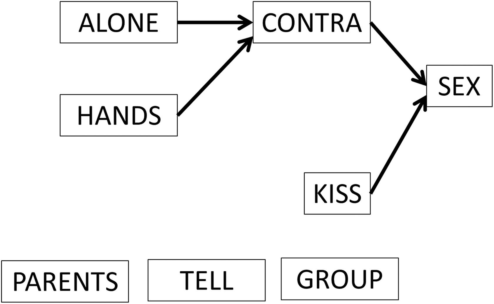
Poset common to all 80 patterns.

The first group (see Figure 5a) appears to work on a logic of privacy—it is only right before the “contraception talk” that the partner is introduced to parents and that friends are told about the relationship. In stark contrast, in group 5b (predominantly girls), after a group date, friends would be told about the relationship, possibly even before the two had even been on a date together. In contrast, parents would not be told until later. Finally, in Figure 5c, we see a group (predominantly boys) in which physical contact (holding hands and kissing) comes before going out in public, and perhaps even before a formal date.

Figure 5.

Three example groups. (a) “Privacy” includes 37 girls and 22 boys, (b) “groupies” includes 17 girls and 2 boys, and (c) “grabbers” includes 21 girls and 39 boys.

It is of course true that a clustering routine like this will always produce results (the same is true for most sequence-clustering algorithms). However, the fact that the interpretations of the logics of the clusters seem to correlate with the gender composition gives us reason to believe that the results are not arbitrary.

We have demonstrated the utility of conceiving of data on a set of sequences of events as stemming from underlying deterministic partial orders. But this was, as we recall, only one way of relaxing the assumption of a single determinate sequence. The other relaxation is to continue to assume a single order but allow for a stochastic response process. We go on to consider ways of clustering respondents based on this assumption.

Orders and Partial Orders

From Incomparability to Indistinguishability

The hallmark of the approach above was to go from sequences (ordered sets) to partially ordered sets. This makes sense if we find that some events are intrinsically incomparable. But, as said above, partial orderings may arise in sets of responses on the same ordered events if some of the events are difficult to order. In particular, it might be that the events are so close in time that respondents are unable to recall precisely which came before the other. Indeed, there is reason to think that this will hold in the Add Health data; respondents were explicitly told, “Don’t worry if two things happened at the same time. Just pick one to put first, and put the other one after it.”

It is worth emphasizing that these two different cases have very different implications for how we use the data to characterize the events. If the observed data from some group is partially ordered simply because of difficulties in discrimination, the mean rank, and/or its column sum in the X matrix, of any event is likely to be a reasonable approximation for the underlying interval score. Quite different is when respondents assemble substructures that have local orderings that do not give rise to a complete ordering (such as the example above of the events in the American Revolution). In such a case, the rank is not a reasonable approximation for the underlying interval score.

For this reason, we might be interested to see whether the partial orders that characterize some observed group might be seen as reducible to an underlying order. Here, we then propose that our manifest partial ordering, one compatible with a Leibnizian approach to time, is in fact generated by processes that occur in some Cartesian time. For example, it should be obvious upon inspection that both the group of Figure 5a and that of Figure 5b may be expressed as underlying orders, only with some events as indistinguishable (e.g., Kiss and Hands for Figure 5a and Tell, Alone, and Hands for Figure 5b). In contrast, in Figure 5c, it is not obvious that such an order fits the data. If Tell, Parents and Alone are indeed at the same “time” as Group, why are they not preceded by Kiss and Hands? On the other hand, if they are contemporaneous with Kiss and Hands, why do they not precede Group?

To determine this, we must postulate some process linking position in Cartesian time to the observed data. There have been, historically, two ways of doing so. One is to propose that an underlying order will be realized in a respondent’s subjectivity as a partial order if she could not discriminate between items within some “just noticeable difference” (see Martin 2009:174-6)). However, this notion, despite its intuitive plausibility, has less psychological justification than the alternative, first proposed cogently by C. S. Peirce (Peirce and Jastrow [1885] 1993). Peirce’s experimental work suggested that even when a subject was uncertain and did not have confidence in a judgment of ranking between two close cases (e.g., the heavier of two objects of similar weight), the probability of a correct choice increased monotonically with the difference between the two stimuli.

This is the logic that underlies the method of paired comparisons developed later (see David 1988). The logic here is that each case has a position on an interval metric, and the subject makes a comparison between the values of two at a time, tending to prefer the higher one in a stochastic process such that the error of a reversal increases as the two items become closer. The simplest such model is known as the Bradley–Terry model (Bradley 1953, 1965; Bradley and Terry 1952). We go on to explain the application of this model to our data, and present illustrative examples.

A Model for Underlying Orders

Here, our assumption is that respondents who have experienced the same underlying sequence will give different reports because there is only a stochastic, and not deterministic, relation between the true ordering and the response process. When events are far apart in time, the chance of respondents reversing the true order is low. But as the time difference between two events goes to zero, the odds of an error increase. Thus, with a set of data, we can do two things: First, we can test whether or not the hypothesis of a single latent order is plausible, and second, if we accept this model, we can estimate the positions of events in relative time.

For some data, there may well be pairs of events that have a strong precedence relation in the data even though they were temporally close together. Those who gave birth before getting married are not likely to forget this ordering, even if the two were quite close. In such cases, the method here may still produce useful results, interpreted less as estimates of calendar time and more of a social time (Zerubavel 2003).

For any subset of respondents S, we can compute a K × K matrix X ^S with values as follows:

x_{j k}^{S} = \sum_{i \in S} In (z_{i j} < z_{i k}) .

This is the number of persons within S who rank item j before item k. Note that x^S _jk + x^S _kj = N_S = |S|. Imagine that every event has some position along a temporal ordering (which we denote a^S _j for the jth event), even though not all respondents know exactly where. We may propose that the logodds that a respondent in S places event j before event k is a linear function of the difference between these two individuals in terms of this underlying position. Thus, we say:

ln [\frac{x_{j k}^{S}}{x_{k j}^{S}}] = a_{j}^{S} - a_{k}^{S} .

This is equivalent to the Bradley–Terry model for paired comparisons (Bradley 1953, 1965; Bradley and Terry 1952). Because only differences between the a parameters are meaningful, one arbitrary restriction must be placed on them; accordingly, they are constrained to sum to zero. This model can be fitted as a logistic regression using a standard statistical package given the proper design matrix.

In some cases, a model will not converge under conventional maximum likelihood estimation because it fits perfectly, that is, the case for the posets in Figure 5a and b. The model correctly identifies that there are strata of events (five for the first example, and six for the second), but the fitting routine will, to maximize the predicted odds in equation (4), spread the times out further and further, until some overflow error is reached. For this reason, we use a “bias-reducing” maximum likelihood (Firth 1993), which ensures finite estimates.⁵

Given that large distances between event times ({a^S _k, k = 1…K}) indicate more perfect prediction, the degree to which these times are spread out indicates the degree to which the partial order is compatible with a stochastic process on a latent order. For this reason, the standard deviation of {a^S _k}, denoted σ ^S _k , can be used to measure the degree of consensus on the ordering of elements by the members of S. For example, if we were to have two sets, S and S′, with the same number of members, and σ ^S _k > σ ^S ^′ _k , we would conclude that the members of S are in greater agreement than the members of S′. This can be used to see not only whether, for example, boys agree more than do girls, but whether boys and girls tend to disagree. This last would be determined by seeing whether mixed groups of a random selection of N*/2 boys and N*/2 girls has a lower σ ^S _k than does a sample of either N* boys or N* girls, where N* = min(N^boys, N^girls).

In contrast to cases where the Bradley–Terry model fits perfectly, consider the poset displayed in Figure 6. This is a fourth cluster from the six reached by our partial order clustering algorithm. In this case, although the Bradley–Terry model drastically increases the fit over the null model containing only a constant (6,153.01 χ² points for 7 df, p < .001), the deviance from the model is highly significant (411.99 χ² points with 21 df; p < .001) and therefore we would reject the hypothesis of an underlying order. It is clear that in this group, the reason for the rejection is that they are certain that parents should be told before the relation gets serious, but they are undecided about the involvement of the peer group.

Figure 6.

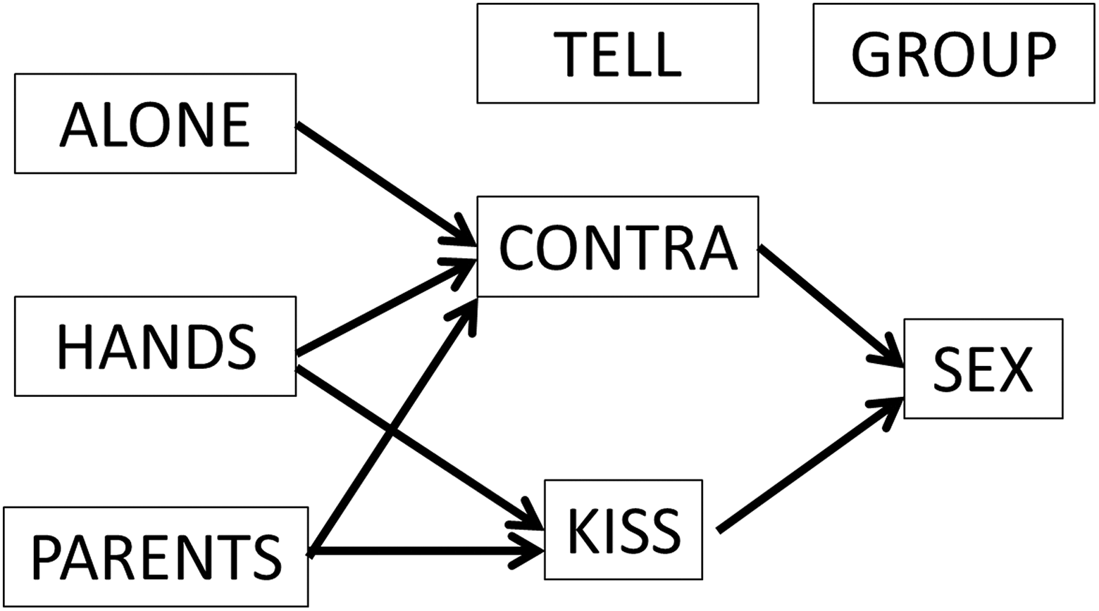
A fourth cluster. This includes 70 girls and 101 boys.

In sum, it is possible that the algebraic approach, which focuses on manifest partial orders, is compatible with the hypothesis of a latent complete order. For some data sets, any prejudice in favor of a complete order would be quite unjustified. For example, when it comes to the “ideal structures” of dating, there may be strong preferences for the ordering of certain pairs of events (e.g., whether talk about contraception happens before or after first intercourse), but not for others. However, in other cases, especially where multiple respondents are reporting on the same set of transpired events, we might be interested in testing the global model of a single order for all respondents. And there may be other cases in which we are interested in determining whether there may be alternate stochastic orders, which produce, on aggregate, posets that seem to fall short of complete ordering. We go on to explore this possibility.

Clustering for Orders

In this case, we might seek to uncover clusters in our data of respondents who share an underlying latent order, even if their manifest orders are different. Thus, we might, in constructing clusters, give preference to groupings that would be like Figure 5a or b over ones like that displayed in Figure 5c, and we would find a cluster like that displayed in Figure 6 quite unacceptable.

It might seem that we could use the Bradley–Terry test as a criterion for such combinations, but because the model will tend to fit many “low N” posets exactly, and small cell counts make statistical tests inappropriate, this is not a plausible choice for all stages of a clustering algorithm. Instead, we propose a more ad hoc but intuitive penalty function, which guides the algorithm to cluster rows that are more likely to lead to a subset of data compatible with a Bradley–Terry model.

Let c_j be the total of the jth row of X ^S , and let M(S) be {j | c_j = min}; that is, it is all the elements in the poset that do not precede any other elements (this includes isolated elements that have no precedence relations with any other elements). For example, in Figures 5a−c, Sex is the only minimal element. Construct for each element a score t_j such that t_j is the minimum of the path lengths from j to all members of M(S). Thus, in Figure 5c, the score for Sex would be 0, that for Contra, 1, that for Tell, Group, Parents, and Alone, 2, and that for Kiss and Hands, 3. Construct a matrix B ^S which is the Boolean version of X ^S ; that is, b^s _ij = 1 iff x^s _ij > 0. Now consider the following ad hoc penalty function P(s):

P (S) = {(N_{S})}^{g} \sum_{i, j > i} [1 - (1 - {b^{s}}_{i j}) (1 - {b^{s}}_{j i})] | t_{i} - t_{j} | .

This in effect adds the difference in rank between any two events if there not a precedence relation between the two. Thus, for Figure 5c, the lack of a precedence relation between Tell and Group would not increase the penalty function because they have the same score; the difference in score between Kiss and Contra would not increase the penalty function because Kiss precedes Contra. However, the lack of relations between Kiss and Hands on the one hand and Tell, Parents, and Alone on the other would lead to a total score of 6.

We then use the same agglomerative technique to produce a hierarchical clustering object. (The same principles of weighting each pattern by the number of occupants therefore apply here as well.) However, we now have a potential statistical criterion for where we make the otherwise arbitrary cuts: We begin at the “top” and test the Bradley–Terry model for a latent order. If this is rejected, we then progress backward through the dendogram, seeing when we can cease splitting clusters, because we determine that the Bradley–Terry model is an adequate characterization of the data.

Example

Here, we again use the public Add Health data, though this time, rather than look at the ideal events that respondents list, we look at the actual ordering of events among the 555 white non-Hispanics who experienced all eight of these steps in their first named wave 2 relationship. Unlike the ideal sequences, the real sequences are the outcome of a joint production, sometimes a compromise or emergent order, of two persons, and may perhaps lack the clarity of the structure of the “scripts” that each person might have independently. Thus, the stochastic order model may be more appropriate here, and the partial order model more appropriate for ideal sequences. Once again, we eliminate all the observations that are unique, leaving us with a total N of 280, although given that we have a stochastic model for the response process, the results are far less sensitive to the inclusion of rare patterns than when we use a nonstochastic version, such as that employed above.⁶

In applying our routine, we consider ourselves to have identified a cluster sharing a linear script when we fail to reject the Bradley–Terry model using a classical test of the residual deviance at p < .05. Although this might seem a generous criterion (since failure to reject is not the same as to accept), because given our 8 steps, each respondent contributes 8 × 7/2 = 28 observations, the total χ² may be seen to be overly conservative. It is of course possible to do more complex tests for the Bradley–Terry model, including those that take into account the number of “raters” (here, respondents), but for our demonstrative purposes, we use a simple test. Other criteria, such as information-theoretic or Bayesian model selection criteria, or proportional reduction of error, might also be used. As noted above, because of problems coming from perfect predictions, we use the “bias-reducing” estimator incorporated in the R package BradleyTerry2 (Turner and Firth 2012).

Our algorithm produces nine different linear orders, with 85, 53, 45, 28, 23, 22, 8, 8, and 8 members each. Figure 7 displays the six of these with the most members, with those higher having more members than those low. It will be noted that in all of the cases, Sex is the terminal element. This was not the case in the data as a whole, where 121 of the 555 cases had Sex coming before the final stage. However, these patterns were all rejected as singletons. It might be that there is not a consensual script in which sex is nonterminal, and hence these sequences are better interpreted as a lack of structure than any particular structure.

Figure 7.

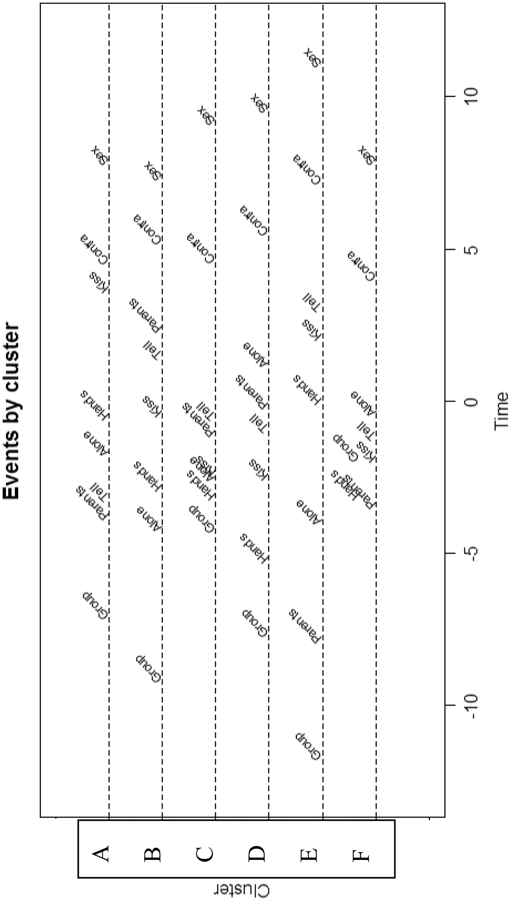
Linear clusters.

The pattern on top (A) has a separation between group participation, presexual friendship, and then escalation to sex. The next pattern (B) is quite similar, but with a major difference in the position in which parents were notified—while this comes quite early in the first sequence, it is quite later in the second. Telling friends follows parents in both cases. It is worth pointing out that while it takes two to have a romantic event sequence, there are two types of objective disagreement possible in these data. One party can tell his or her friends while the other does not, and the same goes for parents. It is perhaps interesting that 59 percent of those in the first sequence, with telling Parents early, are girls, while only 41 percent in the second cluster are.

The third sequence (C) is more like the second, but the events are more compressed and kissing comes somewhat earlier. The fifth (E) sequence, with 23 observations, is marked by a very clear separation or equivalently, high agreement on the ordering, which starts with being in a group and telling parents early, which may also be suggestive of a very strict script.

It is interesting that here we see divisions among respondents that are, in substantive terms, similar to those we saw when analyzing ideal sequences. There is a split between those who place parental communication early, those who place group involvement early, and those who hold off on both of these until the relation is more serious. This internal validity is reassuring that the approaches are not producing meaningless clusters and inciting irresponsible interpretations.

An Addendum on Measured Posets

All our approaches have been for cases in which the data come in the form of observed sequences; our clustering that looks for latent orders assumes that the observed differences between responses in a cluster come from the difficulty of discriminating between events that took place close together in experiential time. It is, however, worth noting that if we were to have observed data on a partial ordering from such a group, we could decompose it into a set of different underlying orders using an algebraic factorization. In other words, we determine a realizer of the observed poset A as the set of linear extensions that recreates A. For example, imagine that a group was set to work to order pairs of events, and rules of consensus led them to produce a partial ordering. (In other words, though all participants had orders of the events, the final structure only included relations between elements that all agreed on.) We then attempt to uncover the orderings that realize A.

Although there may be multiple sets of possible realizers of any poset, we can compute the dimensionality of the poset as the number of minimal orders that jointly realize the poset. This is computationally not easy and involves the construction of a hypergraph from the incomparability matrix (Felsner and Trotter 2000). But as an example, take the connected component of Figure 4, the portion of the poset involving Alone, Hands, Contra, Kiss, and Sex. This partial order has width 3, but the dimensionality is actually only 2, as the following two linear extensions of the poset are sufficient to realize it: {Kiss, Alone, Hands, Contra, Sex} and {Hands, Alone, Contra, Kiss, Sex}. Of course, given data that come in the form of sequences, there is no need to re-create such sequences from the partial orders; even given data on observed partial orders, such recreation is likely to be difficult, as the number of distinct possible realizers can be quite large, but we point this out for purposes of completion.

Conclusion

The study of the relations between events can be quite difficult, even in the best of (Cartesian) times. Existing techniques for sequence analysis have deliberately attempted to fuse four types of differences in event sequences: differences of attainment (i.e., where events are ordered, the maximum attained), differences of sequence length, differences of sequence content, and differences of ordering. We believe that this has led our techniques to increase, as opposed to decrease, ambiguity regarding what sorts of differences are actually being captured.

A second form of ambiguity enters because, in some cases, respondents may actually have an underlying partial order, but be required to report a strict order. In such cases, aggregating cases to find similarities may be necessary for us to understand the actual logic used by respondents. In other cases, however, respondents may experience a true underlying order but may only have a stochastic response process link this experienced order to the reported one. In such cases, we may find that the use of stochastic models for latent orders, applied to aggregate data that take the form of partial orders, may be better at reproducing respondents’ actual ordering of the items than their manifest response. Further, this gives a statistical criterion that can be used to control the behavior of clustering routines, should we have a priori reason to believe that the underlying data were ordered.

The methods developed here require that all observations be expressable as permutations of the same set of unique (nonrepeated) objects (in this case, events). Where this loses too much information because, for example, few respondents share a set of events, or events are repeated, other methods will be preferable. In other words, to the extent that our data approaches a permutation of a set, the approaches laid our here are promising. When do we have such data? For one, when respondents are actually asked to order events, as in Yeatman and Trinitapoli (2017); for another, when they order nonevents, such as ranking tasks (e.g., Rokeach 1973).

More generally, however, we are often interested in “nonrecurrent” events. One theoretically intriguing class of such events are “firsts” (e.g., first alcohol use and first intercourse). A related set are transitions associated with adulthood (gainful employment, moving out, marriage, and childbirth). Where we are interested in comparing across subjects not all of whom have experienced all events, we might be interested in the approach of Billari and Piccarreta (2005). But if we are interested in examining a set of persons, all of whom have completed all transitions, the methods here might be preferable. And, of course, if our sequences varied in the content, or if there were repeated events, we might prefer the approach of Elzinga (2003).

In sum, the methods introduced here have the typical strengths and weaknesses of mathematical approaches—they have a clearer theoretical relation to the ideas driving our research than do ad hoc procedures, but at the cost of fragility or greater demands on the data. We have argued that such limitations allow us to focus on what is theoretically most central to the notion of the form of sequence. In particular, our approach is targeted to one special class of events where all participants experience a fixed set of nonrecurrent events. We hope that the development of techniques that sacrifice breadth of application for the theoretical cogency of their assumptions can help formal techniques for event sequences attain a degree of conceptual precision to match other statistical techniques.

Supplemental Material

Supplementary_material_(1) - Some Methods for the Analysis of Event Sequence Data from Multiple Respondents

Supplementary_material_(1) for Some Methods for the Analysis of Event Sequence Data from Multiple Respondents by John Levi Martin and James P. Murphy in Sociological Methods & Research

Footnotes

Authors’ Note

An earlier version was presented at the conference on Networks and Events, Yale Institute for Network Science, September 16, 2016.

Acknowledgments

We thank the organizers, Emily Erickson, Marissa King, and Balazs Kovacs, as well as Peter Bearman and Ronald Breiger, for their support and comments. And we are extremely grateful to Jenny Trinitapoli for a close reading and comments that greatly improved this article. This research uses data from Add Health, a program project directed by Kathleen Mullan Harris and designed by J. Richard Udry, Peter S. Bearman, and Kathleen Mullan Harris at the University of North Carolina at Chapel Hill, and funded by grant P01-HD31921 from the Eunice Kennedy Shriver National Institute of Child Health and Human Development, with cooperative funding from 23 other federal agencies and foundations. Special acknowledgment is due Ronald R. Rindfuss and Barbara Entwisle for assistance in the original design. Information on how to obtain the Add Health data files is available on the Add Health website (). No direct support was received from grant P01-HD31921 for this analysis.

Declaration of Conflicting Interests

The author(s) declared no potential conflicts of interest with respect to the research, authorship, and/or publication of this article.

Funding

The author(s) received no financial support for the research, authorship, and/or publication of this article.

Supplemental Material

Supplemental material for this article is available online.

Notes

References

Abbott

Andrew

. 1998. “The Causal Devolution.” Sociological Methods and Research 27:148–81.

Abell

Peter

. 1993. “Some Aspects of Narrative Method.” Journal of Mathematical Sociology 18:93–134.

Aisenbrey

Silke

Fasang

Anette

. 2017. “The Interplay of Work and Family Trajectories over the Life Course: Germany and the United States in Comparison.” American Journal of Sociology 122:1448–484.

Barban

Nicola

Billari

Francesco

. 2012. “Classifying Life Course Trajectories: A Comparison of Latent Class and Sequence Analysis.” Applied Statistician 61:765–84.

Bearman

Peter

Faris

Robert

Moody

James

. 1999. “Blocking the Future: New Solutions for Old Problems in Historical Social Science.” Social Science History 23:501–33.

Billari

Francesco C.

Fürnkranz

Johannes

Prskawetz

Alexia

. 2006. “Timing, Sequencing and Quantum of Life Course Events: A Machine Learning Approach.” European Journal of Population 22:37–65.

Billari

Francesco C.

Piccarreta

Raffaella

. 2005. “Analyzing Demographic Life Courses through Sequence Analysis.” Mathematical Population Studies 12:81–106.

Bradley

Ralph A.

1953. “Some Statistical Methods in Taste Testing and Quality Evaluation.” Biometrics 9:22–38.

Bradley

Ralph A.

1965. “Another Interpretation of a Model for Paired Comparisons.” Psychometrika 30:315–18.

10.

Bradley

Ralph A.

Terry

Milton E.

. 1952. “Rank Analysis of Incomplete Block Designs: I. The Method of Paired Comparisons.” Biometrika 39:324–45.

11.

Breiger

Ronald L.

Smith

Julia G.

. 2018. “Insurgencies and Networks of Event Orderings.” Sociological Theory 36: 201–209.

12.

Coombs

Clyde H.

1964. A Theory of Data. New York: John Wiley.

13.

Cornwell

Benjamin

. 2015. Social Sequence Analysis. New York: Cambridge University Press.

14.

Cornwell

Benjamin

Warburton

Elizabeth

. 2014. “Work Schedules and Community Ties.” Work and Occupations 41:139–84.

15.

Coxon

Anthony P. M.

Jones

Charles L.

. 1978. The Images of Occupational Prestige. New York: St. Martin’s Press.

16.

David

H. A.

1988. The Method of Paired Comparisons. 2nd ed. London, England: Charles Griffin.

17.

Elzinga

Cees H.

2003. “Sequence Similarity: A Non-aligning Technique.” Sociological Methods and Research 32:3–29.

18.

Elzinga

Cees H.

2005. “Combinatorial Representations of Token Sequences.” Journal of Classification 22:87–118.

19.

Elzinga

Cees H.

2010. “Complexity of Categorical Time Series.” Sociological Methods and Research 38:463–81.

20.

Fasang

Anette Eva

Liao

Tim Futing

. 2014. “Visualizing Sequences in the Social Sciences: Relative Frequency Sequence Plots.” Sociological Methods & Research 43:643–76.

21.

Felsner

Stefan

Trotter

William T.

. 2000. “Dimension, Graph and Hypergraph Coloring.” Order 17:167–77.

22.

Firth

David

. 1993. “Bias Reduction of Maximum Likelihood Estimates.” Biometrika 80:27–38.

23.

Frye

Margaret

Trinitapoli

Jenny

. 2015. “Ideals as Anchors for Romantic Experiences.” American Sociological Review 80:496–525.

24.

Gagnon

John H.

Simon

William

. 1973. Sexual Conduct. Chicago, IL: Aldine.

25.

Guttman

Louis

. 1950. “The Basis for Scalogram Analysis.” Pp. 60–90 in Measurement and Prediction, Studies in Social Psychology in World War II, Volume IV, edited by Stouffer

Samuel A

Guttman

Suchman

Edward A.

Clausen

John A.

. Princeton, NJ: Princeton University Press.

26.

Halpin

Brendan

. 2010. “Optimal Matching Analysis and Life-course Data: The Importance of Duration.” Sociological Methods & Research 38:365–88.

27.

Harding

David J.

2007. “The Cultural Context, Sexual Behavior, and Romantic Relationships in Disadvantaged Neighborhoods.” American Sociological Review 72:341–64.

28.

Hollister

Matissa

. 2009. “Is Optimal Matching Suboptimal?” Sociological Methods & Research 8:235–64.

29.

Martin

John Levi

. 2009. Social Structures. Princeton, NJ: Princeton University Press.

30.

Moody

James

. 2002. “The Importance of Relationship Timing for Diffusion: Indirect Connectivity and STD Infection Risk.” Social Forces 81:25–56.

31.

Paik

Anthony

Woodley

Vernon

. 2012. “Symbols and Investments as Signals: Courtship Behaviors in Adolescent Sexual Relationships.” Rationality and Society 24:3–36.

32.

Peirce

Charles S.

Jastrow

. [1885] 1993. “On Small Differences of Sensation.” Pp. 122–35 in Writings of Charles S. Peirce, volume 5, edited by Christian

J. W. Kloesel

. Bloomington, IN: Indiana University Press.

33.

Pretzel

Oliver

. 1977. “On the Dimension of Partially Ordered Sets.” Journal of Combinatorial Theory A 22:146–52.

34.

Rasch

Georg

. 1966. “An Individualistic Approach to Item Analysis.” Pp. 89–107 in Readings in Mathematical Social Science, edited by Lazarsfeld

Paul F.

Henry

Neil W.

. Cambridge: MIT Press.

35.

Rokeach

Milton

. 1973. The Nature of Human Values. New York: Free Press.

36.

Smith

Tammy

. 2007. “Narrative Boundaries and the Dynamics of Ethnic Conflict and Conciliation.” Poetics 35:22–46.

37.

Soller

Brian

. 2014. “Caught in a Bad Romance: Adolescent Romantic Relationships and Mental Health.” Journal of Health and Social Behavior 55:56–72.

38.

Soller

Brian

. 2015. “I Did Not Do It My Way: The Peer Context of Inauthentic Romantic Relationships.” Sociological Perspectives 58:337–57.

39.

Stovel

Katherine

Savage

Michael

Bearman

Peter

. 1996. “Ascription into Achievement: Models of Career Systems at Lloyds Bank, 1890–1970.” American Journal of Sociology 102:358–99.

40.

Thomas

William I.

Znaniecki

Florian

. 1918. The Polish Peasant in Europe and America, Volume I: Primary-group Organization. Boston, MA: Gorham Press.

41.

Trotter

William T.

1992. Combinatorics and Partially Ordered Sets: Dimension Theory. Baltimore, MD: Johns Hopkins University Press.

42.

Turner

Heather

Firth

David

. 2012. “Bradley–Terry Models in R: The BradleyTerry2 Package.” Journal of Statistical Software 48:1–21.

43.

Warren

John Robert

Luo

Liying

Halpern-Manners

Andrew

Raymo

James M.

Palloni

Alberto

. 2015. “Do Different Methods for Modeling Age-graded Trajectories Yield Consistent and Valid Results?” American Journal of Sociology 120:1809–856.

44.

Wiley

James

Martin

John Levi

. 1999. “Algebraic Representations of Beliefs and Attitudes: Partial Order Models.” Sociological Methodology 1999:113–46.

45.

Lawrence

. 2000. “Some Comments on ‘Sequence Analysis and Optimal Matching Methods in Sociology: Review and Prospect.’” Sociological Methods and Research 29:41–64.

46.

Yeatman

Sara

Trinitapoli

Jenny

. 2017. “Awareness and Perceived Fairness of Option B+ in Malawi: A Population-level Perspective.” Journal of the International AIDS Society 20:21467.

47.

Zerubavel

Eviatar

. 2003. Time Maps. Chicago, IL: University of Chicago Press.

Supplementary Material

Please find the following supplemental material available below.

For Open Access articles published under a Creative Commons License, all supplemental material carries the same license as the article it is associated with.

For non-Open Access articles published, all supplemental material carries a non-exclusive license, and permission requests for re-use of supplemental material or any part of supplemental material shall be sent directly to the copyright owner as specified in the copyright notice associated with the article.

0.00 MB

0.16 MB